Conductor Temperature Monitoring of High-Voltage Cables Based on Electromagnetic-Thermal Coupling Temperature Analysis

Abstract

As a key state parameter of high-voltage cables, conductor temperature is an essential determinant of the current carrying capacity of cables, but in practice, this is difficult to measure directly during the operation of high-voltage cables. In this paper, the electromagnetic-thermal coupling analysis model of a 110 kV high-voltage cable is established using the finite element analysis software COMSOL. By analyzing the temperature distribution law of high-voltage cables under different load currents and ambient temperatures, the relationship between the change in the high-voltage cable surface temperature and the conductor temperature is deduced, which allows the monitoring of the high-voltage cable conductor temperature. Taking the 110 kV cable of the Yanzhong line in Shanxi Province as an example and using the electromagnetic-thermal coupling temperature field analysis method, the conductor temperature of the high-voltage cable can be measured using the data obtained from the cable surface temperature, which is measured by the self-developed Raman Distributed Temperature Sensor (RDTS) system with a maximum measurement error of about 2 °C. The method is easy to use and can achieve the accurate measurement of the conductor temperature without damaging the cable body.

1. Introduction

Along with the development of smart grids, the stable operation of high-voltage cables, as important carriers of electric power transmission, is conducive to guaranteeing the quality of a power supply and improving the safety and reliability of power transmission lines [1,2,3]. The conductor temperature of high-voltage cables is one of the important parameters that directly determine their load capacity [4,5]. Without a comprehensive consideration of the actual operating environment of high-voltage cables, a rise in conductor temperature that exceeds the allowable value will accelerate the aging of the cable insulation, increase the leakage current, and eventually lead to insulation breakdown. Therefore, the monitoring of the temperature of cable conductors is significant for assessing the real-time load capacity of cables and ensuring their stable and efficient operation.

In recent years, the development of online monitoring technology for high-voltage cable surface temperature has become the basis for the calculation of high-voltage cable conductor temperature. The common methods for monitoring the temperature of the cables can be divided into non-contact and contact temperature measurements. As a representative of non-contact temperature measurement, infrared temperature measurement technology has a faster response time and simple equipment structure, but it will be affected by infrared electromagnetic waves and environmental factors radiating from non-measurement objects, resulting in poor measurement accuracy. Therefore, this method requires the noise reduction processing of the infrared imaging to obtain accurate temperature information [6,7]. In contact temperature sensors, thermocouple sensors are often used for multi-point measurements [8,9]. Compared to infrared temperature measurement, the arrangement is flexible and allows temperature measurement at multiple locations, but it is not easy to maintain a safe electrical distance between the point sensors and equipment with high voltage levels. Therefore, neither method is the most suitable choice for the continuous long-distance monitoring of the temperature of cable lines in complex laying environments. The distributed fiber optic temperature measurement (DTS) system lays the fiber on the cable surface or builds the fiber into the cable and uses the scattering characteristics of laser propagation in the fiber to achieve the distributed measurement of the temperature field [10,11,12,13]. The DTS has good insulation performance, high sensitivity, and long transmission distance; therefore, the DTS can meet both the long-distance monitoring demand and obtain accurate temperature information for the online monitoring of long-distance and high voltage level cables without the interference of the electromagnetic environment.

The above methods are usually used to detect the surface temperature of high-voltage cables, but the direct measurement of the conductor temperature of the cable is difficult to achieve. At present, the main estimation methods for the conductor temperature of power cables include the equivalent thermal circuit models [14,15], artificial intelligence algorithms [16], and finite element analysis [17,18,19]. IEC 60287 is the standard for the equivalent thermal circuit method, which provides a complete analysis method and formula for calculating the load capacity [20]. However, this calculation method does not consider the influence of changes in the external environment and other factors on the correction coefficient [21] and cannot effectively solve physical problems, such as air convection, radiation, and heat transfer coupling. The calculation will generate errors that make the final results deviate from the actual values in multi-loop and complex environments. Therefore, it is not suitable for the real-time temperature monitoring of conductors. In addition, artificial intelligence algorithms have also been applied to the prediction of the temperature of cable conductors. By using support vector machines (SVM), the transient temperature model of the conductor is established and a particle swarm optimization (PSO) algorithm is introduced to optimize the network model parameters. The measured cable surface temperature and load current are used as model inputs to obtain the dynamic temperature of the conductor [22], but in order to use this method, a large amount of sample data is required to train the conductor temperature calculation model. The finite element method (FEM) can study the continuous solution domain by dividing it into a finite number of individual units, depending on the different scenarios, and multi-physics field coupling calculations can be performed for complex structures. A three-dimensional multi-field coupling analysis model for the cable and joint is established and the distributions of electromagnetic and temperature fields are calculated according to the boundary conditions in COMSOL [23,24]. However, most simulation models do not take into account the temperature distribution in the case of simultaneous changes in each parameter.

In this paper, a non-invasive method for calculating the conductor temperature of high-voltage cables is proposed, based on the electromagnetic-thermal coupling temperature analysis method. A simulation model of the cable trench is established in FEM software COMSOL according to the actual situation, and the effect of simultaneous changes in ambient temperature and load current on the temperature is analyzed in the electromagnetic-thermal coupling field. An analytical formula is derived to calculate the conductor temperature by extracting the change law of the cable surface temperature and the conductor temperature in the simulation model. The feasibility of the method to obtain the cable conductor temperature indirectly through the model is verified by using the RDTS system to obtain multiple sets of cable surface temperature data under different operating conditions.

2. Theoretical Model

The operation of power cables mainly involves the coupling calculation of electromagnetic and thermal fields. The electromagnetic loss after applying the load current to the cable causes the cable to heat up and that temperature increase affects the conductivity of the cable conductor. When performing the electromagnetic-thermal coupling solution for high-voltage cables, the following assumptions are made to facilitate the calculation:

(1) The displacement current can be excluded when the high-voltage cable is operated at power frequency (50 Hz) because the conductive current density is much greater than the displacement current density;

(2) In addition to the conductivity of the copper conductor, the other component materials of the cable are considered isotropic homogeneous mediums and the physical parameters of each part are constant;

(3) The simulation only investigates the steady-state distribution of the conductor temperature of the high-voltage cable and thus, the control equation does not contain a time term.

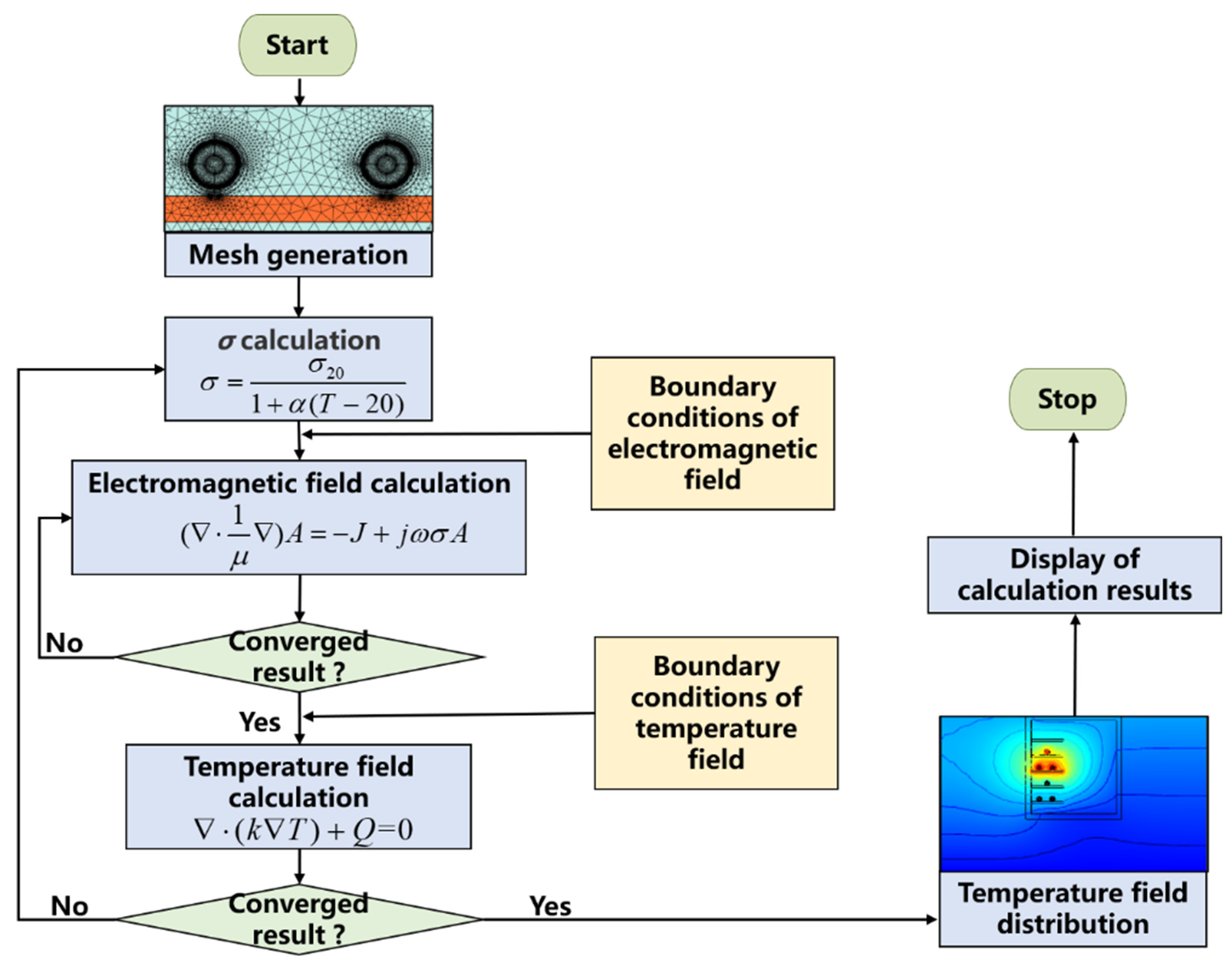
The theoretical model is shown in Equations (1)–(4). Based on the above assumptions and Maxwell’s equations, the control equations of the electromagnetic field in the temperature field solution are shown in Equation (1). According to Fourier’s law, the losses generated by the cable will be converted into heat without considering the external heat source, thus increasing the temperature of the cable and the surrounding medium. Equation (2) describes this temperature increase process. The conductivity of the cable conductor decreases with the increase in temperature, and the relationship between its conductivity and temperature is shown in Equation (3) [22]. Equation (4) indicates that in temperature field calculations based on the law of energy conservation, the heat source in high-voltage cables mainly comes from Joule losses due to conductor currents.

$$(\nabla \cdot \frac{1}{\mu }\nabla )A=-J+j\omega \sigma A$$

(1)

$$\nabla \cdot (\lambda \nabla T)+Q=0$$

(2)

$$\sigma =\frac{{\sigma }_{20}}{1+\alpha (T-20)}$$

(3)

$$Q=\frac{1}{\sigma }{\left|J\right|}^2$$

(4)

where: μ is the material permeability, H/m; J is the current density, A/m³; A is the magnetic vector potential, Wb/m; σ is the material conductivity, S/m; ω is the angular frequency, rad/s; T is the temperature, K; λ is the thermal conductivity of the material, W/(m·K); Q is the heat generated per unit volume inside the object (electromagnetic loss density), W/m³; ${\sigma }_{20}$ is the conductor conductivity at 20 °C, S/m; and α is the temperature coefficient, 1/K.

For high-voltage cables, the boundary conditions corresponding to the electromagnetic field on the surface and cross sections on both sides can be expressed as:

$$A=0$$

(5)

$$n\times A=0$$

(6)

where n is the normal vector of the cross sections on both sides.

In the temperature field simulation, the cable trench and the outer soil region are taken as the solution domain and there are four boundaries to be constrained. The upper boundary is the contact surface of the soil and the top of the cable trench with the ground air, which is used as the ambient temperature to dissipate heat to the outside air region by natural convection using the convective heat transfer boundary condition as shown in Equation (7). The lower boundary is a deep layer of soil, and a constant temperature boundary condition is set as shown in Equation (8). The normal temperature gradient of the soil layer at the left and right boundaries is 0. The heat balance boundary condition is set as shown in Equation (9).

$$-\lambda \frac{\partial T}{\partial n}=h(T-T_{amb})$$

(7)

$$T=T_c$$

(8)

$$\lambda \frac{\partial T}{\partial n}=0$$

(9)

where: h is the convective heat transfer coefficient, W/(m²·K); T_amb is the ambient temperature, K; and T_c is the deep soil temperature, K.

A double iterative algorithm is used for the numerical calculation of the simulation model and the calculation flow is shown in Figure 1.

To obtain the temperature distribution under different ambient temperatures and load currents and to further analyze the temperature relationship between the cable skin and the conductor, a 3D model of the electromagnetic-thermal coupling was established in the finite element analysis software COMSOL, based on the cable trench of the Yanzhong Line in Yuncheng City, which is discussed later. In the study of the temperature distribution of the cable body, a section in the middle of the cable with a length of about 10 m, which was almost immune to the heat generation caused by the termination contact resistance, was modeled and simulated and there was almost no temperature variation in the axial direction at steady state. Figure 2a shows the distribution of the Yanzhong line and Figure 2b shows the structure of a 110 kV high-voltage cable, which mainly includes the: conductor; conductor shield; XLPE insulation; insulation shield; waterproof layer; air layer; corrugated aluminum sheath; and outer sheath. It is considered that the conductivity and structural properties of each part of the material remain constant and do not change with the temperature when ignoring the uneven distribution of the air layer due to gravity and external forces, except for the conductor. The material properties and dimensions of each part are shown in

Table 1. The physical dimensions and material parameters of the 110 kV cable.

Layer	Layer Thickness (mm)	Thermal Conductivity (W·(m·K))	Conductivity (S/m)
Conductor	13	400	5.9 × 107
Conductor shield	1.7	0.66	1 × 10−5
XLPE insulation	17	0.46	1 × 10−18
Insulation shield	1.2	0.65	2 × 10−5
Waterproof layer	2.2	0.09	2 × 10−4
Air layer	0.5	0.03	0
Corrugated aluminum sheath	7	218	4 × 107
Outer sheath	6	0.41	1 × 10−18

.

In practice, the soil around the cable trench is an infinite area and only the soil near the wall of the cable trench will have drastic temperature changes, while temperature changes in the distance can be ignored. Therefore, according to the actual engineering experience, a rectangular area with a length of 4 m and a height of 3 m near the cable trench was selected as the outer soil area.

3. Simulation Results

3.1. Temperature Distribution of Cable Trench

3.1.1. Influence of Ambient Temperature

The temperature T_amb near the ground surface varies considerably with the change of seasons when the cable trench is in a relatively isolated underground environment. When the cable is in operation, different ambient temperatures affect the temperature exchange between the cable trench and the outside world, and its temperature distribution also changes. The temperature distribution characteristics of the cable trench and of the cable were studied with different T_amb. The overall temperature distribution of the cable trench was obtained as shown in Figure 3. I was kept as 1000 A and T_amb was taken as 15 °C, 20 °C, 25 °C, 30 °C, 35 °C, and 40 °C.

The cable conductor carries the maximum temperature as the only heat source in the solution domain, and when the ambient temperature T_amb increases, the conductor temperature also increases with a fixed load current loading on the cable conductor. The lowest temperature of the solution domain appeared at the lower boundary of the soil near the cable trench, which was set to a constant temperature boundary condition. As can be seen from Figure 3, the cable had a load current of 1000 A. When the external temperature gradually increased from 15 °C to 40 °C, the maximum temperature of the solution domain increased from 58.553 °C to 83.271 °C. Additionally, we found that when the temperature inside the cable trench rose, natural convection was preferred for heat dissipation. Therefore, due to the accumulation of heat, the temperature near the top of the cable trench rose with the increase in ambient temperature. When the outside temperature was 40 °C, the temperature at the top (53.815) was 37.236 °C higher than the corresponding temperature (16.579 °C) at an outside temperature of 15 °C.

3.1.2. Influence of Load Current

Under the condition of a constant external ambient temperature, the load current I directly affected the heat loss per unit volume of the cable conductor and also indirectly affected the conductor heat loss by influencing the resistivity of the conductor, which caused the change in the temperature field. Therefore, the temperature distribution of the cable trench and of the cable was studied by changing the load current I. The ambient temperature was kept unchanged as T_amb = 20 °C and the load current I was taken as 300 A, 400 A, 500 A, 600 A, 700 A, and 800 A to obtain the overall temperature distribution of the cable trench, as shown in Figure 4.

When the load current was increased, the temperature inside the trench, centered around the cable, also rose; however, the highest temperature in the solution domain still appeared in the cable conductor and did not shift with the change in load current. This is consistent with the conclusion of [6] that the high-temperature region is always distributed around the conductor. As electromagnetic losses are positively correlated with current density, a rise in load current increases the heat production of the cable, but the natural convection environment does not change and the heat exchange process is suppressed, which results in a rising trend in the overall temperature of the cable trench. An increase in load current caused a faster rise in conductor temperature. When the current increased from I = 700 A to I = 800 A, the conductor temperature rose by 6.519 °C, while it only rose by 3.058 °C when the current changed from I = 300 A to I = 400 A.

The overall temperature difference of the solution domain also increased with the rise in load current. When I = 300 A, the conductor temperature was 23.935 °C and the lowest temperature of 10 °C appeared in the deep soil near the lower boundary, meaning that the temperature difference of the solution domain was 13.935 °C. When a load current of 800 A was applied to the conductor, the temperature rose to 47.892 °C, and the temperature difference at this time was 37.892 °C. The isotherm became denser the closer it was to the cable conductor, and the soil around the cable trench only had a weak temperature change and the isotherm was sparse.

3.2. Temperature Distribution of Cable

The cable dissipated heat uniformly outward through the surface under ideal natural convection conditions. A load current of 1000 A was applied to the cable conductor as the only heat-producing source. The temperature distribution and temperature gradient distribution along the radius direction of the cable cross section at an ambient temperature of 25 °C is shown in Figure 5. The highest temperature of the cable conductor was 68.435 °C and the lowest temperature of the cable surface was 40.267 °C, with a decreasing trend along the radius direction. The temperature gradient within the conductor was almost non-existent due to the high thermal conductivity of the copper conductor, and the same occurred in the metal shield layer, which is applicable in almost all cable laying situations [24]. In addition to this, we found that the temperature changes were more drastic at the junction of the different structural layers of the cable. Compared to the temperature distribution curve, the temperature gradient distribution curve shows obvious multiple peaks and the location of those peaks is the location that the cable structure changes, with a large difference in thermal conductivity. The maximum peak location appeared near the radius of 0.035 m, corresponding to the gap between the air layer and the aluminum sheath.

It can be noted from Figure 6 that the temperature distribution of the cable was simulated by considering T_amb and I. The temperature of the cable surface and the conductor both increased with the increase in T_amb and I. The cable conductor temperature rose faster than the surface temperature because of the thermal conductivity of the material and the heat dissipation area. As the thermal conductivity of copper is much greater than that of the outer sheath, and the structure has a small thermal conductivity that bears a greater temperature difference, the result is that the temperature of the outer sheath increased more slowly than that of the conductor. When T_amb = 10 °C, the current increased from 200 A to 1400 A, which resulted in an increase of 101.2 °C in the cable conductor temperature while the cable sheath temperature only increased by 27.4 °C. The temperature difference between the conductor and the surface rose significantly with the increase in I.

4. Experimental Setup

In this paper, a self-developed RDTS system was used for the measurement of the distributed temperature in the cable trench of the Yanzhong line in Yuncheng City, Shanxi Province. Figure 7 shows the temperature monitoring scheme of the RDTS system. The RDTS experimental setup included a high-precision thermostat, a high-speed pulse modulated laser, a wavelength division multiplexer (WDM), two avalanche photodiodes (APD), two electrical signal amplifiers, a high-speed data acquisition card (DAQ), and a host computer. First, a laser pulse (central wavelength 1550.1 nm; pulse width 10 ns; peak power 4 W) generated by a high-speed pulse-modulated laser was pumped into the WDM through the fiber when the RDTS system started to work, and the Raman Stokes and anti-Stokes backscattered light were separated after coupling. After the photoelectric conversion of the two types of backscattered light with different central wavelengths (1450 nm and 1650 nm, respectively) by APD, the weak electrical signals were amplified by amplifiers and acquired by DAQ. Finally, the temperature information was demodulated by the host computer.

5. Experimental Results and Analysis

In the experiment, the cable on the outer side of the second layer was monitored. In Figure 8, the yellow part of the diagram shows the partial layout path of the fiber. On the condition that the sensing fiber was secured next to the cable surface, the fiber connected to the RDTS host was fixed to the cable surface along the axial direction using nylon ties. The total length of the cable measurement section was 100 m and the fixed nodes were spaced at an interval of 1 m.

The results of the distributed measurements of the RDTS system on 11 May 2021 are shown in Figure 9. As can be seen in Figure 9, the load current reached its peak of 163.12 A near 12:00 while the highest measured temperature of 24.29 °C occurred around 14:00, which was due to the hysteresis of heat transfer. With a smaller overall load current and variation, the measurement results were more dependent on the effect of the environment on the cable temperature, so the influence of this hysteresis on the results was considered to be within the margin of error.

The ambient temperature remained almost unchanged between 00:00 and 04:00 while the measured temperature fell as the load current decreased; around 12:00, the ambient temperature fell while the measured temperature rose as the load current increased. Therefore, the measured temperature had a positive correlation with the load current. In addition, the change in load current between 12:00 and 19:00 was slight and the trend of the measured temperature was also correlated with the ambient temperature. The measured temperature was influenced by both the load current and the ambient temperature, which was also consistent with our simulation results.

The cable temperature characteristics under the influence of T_amb and I were studied in the previous section, and the simulation results show that the temperature distribution of the cable varied with these two factors. Therefore, a method of calculating the conductor temperature from the cable surface temperature was studied to improve the accuracy of the cable conductor temperature calculation by considering the effects of environmental factors and load current. The expression of the temperature difference ΔT between T_i and T_o is shown in Equation (10), where the material of the cable conductor is copper, the temperature inside the conductor is uniformly distributed, T_i is the conductor temperature and T_o is the cable surface temperature. The simulation data in Figure 6 were processed by the curve-fitting method and the temperature difference ΔT with different ambient temperatures T_amb, and the load current I could be obtained as described in Equation (11).

$$\Delta T=T_i-T_o$$

(10)

$$\Delta T=-0.13560+0.00074I+0.00231T_{amb}+0.00003I^2+0.00002T_{amb}^2-0.00001I{T}_{amb}$$

(11)

According to Equations (10) and (11), the temperature calculation of the cable conductor was obtained through Equation (12).

$$T_i=\Delta T+T_o$$

(12)

To verify its accuracy, Figure 10 shows the error relationship between the variation curves of the conductor temperature, calculated according to the fitted equation and the conductor temperature obtained from the simulation.

As can be seen from Figure 10, the cable conductor temperature calculated from the above equation was basically consistent with the temperature results obtained from the electromagnetic-thermal coupling simulation, with a maximum error of about 2 °C. The ambient temperature on the day of measurement was low and the load current fluctuated within a small range, with a maximum load current of 200 A. The heat loss generated by the conductor energization was also small. In this case, the heat exchange process was very slight. The influence of the ambient temperature and the variation of the load current worked together to determine the measurement results, leading to an error of only about 2 °C. When the cable was in an unstable environment and the load current continued to rise significantly, the increased heat loss of the cable caused the heat exchange process to intensify, at which point the error might change. In addition, the temperature error increased with the sudden change in load current, which was caused by the time delay in the temperature change between the surface of the cable and the inner conductor.

6. Discussion

In this study, we propose a method for the long-distance temperature monitoring of cable lines using the RDTS system and inferring the core temperature of the cable from the cable surface temperature, which provides a possible solution to the problem of calculating the conductor temperature.

Through the analysis of the theoretical derivation and the experimental procedure, we found that two factors have an impact on the cable conductor temperature calculation. Firstly, there are limitations in the simulation model. In the modeling, the thread-like metal sheath is treated as a hollow cylinder equivalent and the model can be considered to be drawn based on the actual situation. Multi-physical field coupling can be considered, the influence of convection in the model is abstracted as the heat transfer coefficient h, and the overheating of the cable may lead to deformation. Therefore, the flow field and stress field need to be studied in the next step. Some values for the calculations need to be measured practically, which can be attempted in our subsequent work.

The accuracy of the measured temperature is also a factor worth considering. Since heat conduction has hysteresis, which makes the change in temperature lag behind the change in load, the temperature used for the calculation might have deviated from the real value. More measurement tests should be added in subsequent studies to validate the calculated model more fully, especially for cable lines with higher load currents. The installation and environment also affected the measurement results. The data obtained from the measurement were the closest to the actual temperature only when the fiber was fitted closely to the cable surface. As the RDTS system produces Rayleigh scattering light crosstalk, its temperature measurement accuracy also caused uncertainty in the measurement results. In order to improve the accuracy of the temperature measurement, methods for the elimination of Rayleigh scattering through hardware or software needs to be further investigated.

7. Conclusions

In this paper, a high-voltage cable conductor temperature monitoring system based on electromagnetic-thermal coupling temperature field analysis was proposed and tested in the field. The results show that the system was able to achieve the distributed temperature monitoring of the cable surface and calculate the cable conductor temperature under different ambient temperatures and load currents from the surface temperature.

Since the internal temperature change of the cable affected the conductor conductivity, which in turn affected the heat production of the operating cable, an electromagnetic-thermal coupling model for cable trench monitoring sites was established in COMSOL to make the simulation model closer to the real situation. By analyzing the effects of load current and external ambient temperature on the simulation model, it can be seen that both of the variables acted jointly on the temperature distribution and were related to the temperature difference between the cable surface and the conductor. A conductor temperature calculation method based on the temperature difference was proposed to calculate the conductor temperature from the surface temperature whilst considering the environmental factors and load current. The accuracy of the model was compared to that of the finite element model, which showed that the model has good generality. An experiment for cable conductor temperature monitoring based on the RDTS system was designed. The sensing fiber was arranged along the cable in the axial direction using nylon ties to obtain the real-time temperature of the cable surface, and the calculated temperature of the cable conductor was consistent with the simulated results with a maximum error of about 2 °C.

References

1. Cheng, Y.C.; Zhao, L.; Wu, X.T.; Ni, H.; Ding, P.; Li, X.G.; Zhou, X. Statistical analysis of partial discharge faults of HV cables. In Proceedings of the 2020 IEEE Electrical Insulation Conference (EIC), Knoxville, TN, USA, 22 June–3 July 2020. [Google Scholar]
2. Liu, Y.; Lei, T.; Sun, Z.H.; Wang, C.; Liu, T.Y. Application of Distributed Optical Fiber Temperature System in Online Monitoring and Fault Diagnosis of Smart Grid. In Proceedings of the 2012 Asia-Pacific Power and Energy Engineering Conference (APPEEC), Shanghai, China, 27–29 March 2012. [Google Scholar]
3. Diaz-Aguilo, M.; de Leon, F. Adaptive soil model for real-time thermal rating of underground power cables. IET Sci. Meas. Technol. 2015, 9, 654–660. [Google Scholar]
4. Czapp, S.; Szultka, S.; Tomaszewski, A. Design of power cable lines partially exposed to direct solar radiation—special aspects. Energies 2020, 13, 2650. [Google Scholar]
5. Yang, B.; Wu, K.H.; Zheng, Z.J.; Sun, W.; Wang, Y.Q.; Yang, S.Q.; Liang, R.; Feng, L. Study on improving the current carrying capacity of power cable in real-time operating environment. In Proceedings of the China International Conference on Electricity Distribution (CICED), Xi’an, China, 10–13 August 2016. [Google Scholar]
6. Xiong, L.; Chen, Y.H.; Jiao, Y.; Wang, J.; Hu, X. Study on the effect of cable group laying mode on temperature field distribution and cable ampacity. Energies 2019, 12, 3397. [Google Scholar] [CrossRef] [Green Version]
7. Wu, J.Z.; Lin, J.J.; Gao, Z.J.; Lin, H.H.; Li, Q.Q.; Zhang, C.C. A hybrid fourier-wavelet denoising method for infrared image of porcelain sleeve cable terminal using GSM model for wavelet coefficients. In Proceedings of the International Conference on Power System Technology, Guangzhou, China, 6–8 November 2018. [Google Scholar]
8. Yang, L.; Hu, Z.H.; Hao, Y.P.; Qiu, W.H.; Li, L.C. Internal temperature measurement and conductor temperature calculation of XLPE power cable based on optical fiber at different radial positions. Eng. Fail. Anal. 2021, 125, 105407. [Google Scholar]
9. Wang, Z.; Cao, M.; Wang, D.D.; Zhang, S.Q.; Li, X.L. On-Line monitoring of cable trench and cable pit by using metal armored FBG temperature sensors. Int. J. Smart Grid Clean Energy 2013, 2, 119–124. [Google Scholar]
10. Jaros, J.; Papes, M.; Liner, A.; Vasinek, V.; Mach, V.; Hruby, D.; Kajnar, T.; Perecar, F. Temperature measurement inside metallic cables using distributed temperature system. In Proceedings of the International Conference on Photonics Solutions, Hua Hin, Thailand, 6–8 July 2015. [Google Scholar]
11. Chen, K.; Yue, Y.; Tang, Y.J. Research on temperature monitoring method of cable on 10 kV railway power transmission lines based on distributed temperature sensor. Energies 2021, 14, 3705. [Google Scholar] [CrossRef]
12. Zhou, J.; Yao, K.; Huang, X.W.; Sun, G.S.; Zhang, W.J.; Ashtaq, A.; Hao, Y.; Chen, Y. Temperature calculation and measurement on power cable conductor based on equivalent thermal circuit and BOTDA. In Proceedings of the 2019 IEEE International Conference on Environment and Electrical Engineering and 2019 IEEE Industrial and Commercial Power Systems Europe (EEEIC/I&CPS Europe), Univ Genoa, Italy, 10–14 June 2019. [Google Scholar]
13. Cho, J.; Kim, J.H.; Lee, H.J.; Kim, J.Y.; Song, I.K.; Choi, J.H. Development and Improvement of an intelligent cable monitoring system for underground distribution networks using distributed temperature sensing. Energies 2014, 7, 1076–1094. [Google Scholar] [CrossRef] [Green Version]
14. Enescu, D.; Colella, P.; Russo, A. Thermal assessment of power cables and impacts on cable current rating: An overview. Energies 2020, 13, 5319. [Google Scholar]
15. Velasquez, R.M.A.; Lara, J.V.M. New methodology for design and failure analysis of underground transmission lines. Eng. Fail. Anal. 2020, 115, 104604. [Google Scholar]
16. Ruan, J.J.; Zhan, Q.H.; Tang, L.Z.; Tang, K. Real-Time temperature estimation of Three-Core medium-voltage cable joint based on support vector regression. Energies 2018, 11, 1405. [Google Scholar] [CrossRef] [Green Version]
17. Zhao, A.; Gu, L. Study on the temperature distribution of the outer surface of the cable intermediate joint based on ANSYS simulation. In Proceedings of the 2018 IEEE 4th Information Technology and Mechatronics Engineering Conference (ITOEC), Chongqing, China, 20–23 December 2018. [Google Scholar]
18. Mohamed, A.; Gouda, O. Investigations of cable termination thermal analysis under continuous current loading. IET Gener. Transm. Distrib. 2020, 14, 4122–4131. [Google Scholar]
19. Ghoneim, S.S.M.; Ahmed, M.; Sabiha, N.A. Transient thermal performance of power cable ascertained using finite element analysis. Processes 2021, 9, 438. [Google Scholar] [CrossRef]
20. Dubitsky, S.; Greshnyakov, G.; Korovkin, N. Comparison of finite element analysis to IEC-60287 for predicting underground cable ampacity. In Proceedings of the 2016 IEEE International Energy Conference (ENERGYCON), Leuven, Belgium, 4–8 April 2016. [Google Scholar]
21. Borecki, M. A proposed new approach for the assessment of selected operating conditions of the high voltage cable line. Energies 2020, 13, 1–15. [Google Scholar]
22. Niu, H.Q.; Yu, J.; Ye, K.F. Calculation of transient cable conductor temperature based on support vector machine optimized by particle swarm optimization algorithm. In Proceedings of the 2016 IEEE International Conference on High Voltage Engineering and Application (ICHVE), Chengdu, China, 29 December 2016. [Google Scholar]
23. Yang, F.; Cheng, P.; Luo, H.W.; Yang, Y.M.; Liu, H.B.; Kang, K. 3-D thermal analysis and contact resistance evaluation of power cable joint. Appl. Therm. Eng. 2016, 93, 1183–1192. [Google Scholar]
24. Zhang, Y.Y.; Chen, X.M.; Zhang, H.; Liu, J.F.; Zhang, C.H.; Jiao, J. Analysis on the temperature field and the ampacity of XLPE submarine HV cable based on electro-thermal-flow multiphysics coupling simulation. Polymers 2020, 12, 952. [Google Scholar] [CrossRef] [PubMed] [Green Version]
Figure 1. A flow chart of the conductor temperature calculation.
Energies 15 00525 g001
Figure 2. A schematic diagram of the Yanzhong line cable trench structure: (a) the cable distribution diagram; (b) the schematic diagram of a 110 kV cable.
Energies 15 00525 g002
Figure 3. The cable trench temperature distribution at different temperatures Tamb.
Energies 15 00525 g003
Figure 4. The cable trench temperature distribution under different load currents I.
Energies 15 00525 g004
Figure 5. The temperature distribution of the cable: (a) the axial temperature distribution of the cable; (b) the temperature and temperature gradient distribution of the cable section.
Energies 15 00525 g005
Figure 6. The influence of Tamb and I on temperature: (a) the conductor temperature distribution curve; (b) the surface temperature distribution curve.
Energies 15 00525 g006
Figure 7. The experimental setup of the RDTS system.
Energies 15 00525 g007
Figure 8. The cable temperature monitoring site.
Energies 15 00525 g008
Figure 9. The experimental results of the cable temperature monitoring.
Energies 15 00525 g009
Figure 10. A comparison of the cable conductor temperature calculation results.
Energies 15 00525 g010