3.3. Discussion
The economic criteria of an investment are the most significant for the discussion and the final decision. Additionally, the minimum size of the equipment required to efficiently service FCEV is another parameter discussed in this section. Isenstadt and Lutsey [
23] state that most of the governments invest 2–3 Μ
$; however, in their study, they concluded that the overall cost of HRS will drop to 1 M
$ approximately. They estimate that the specific cost of H
2 production fluctuates from 4 to 10
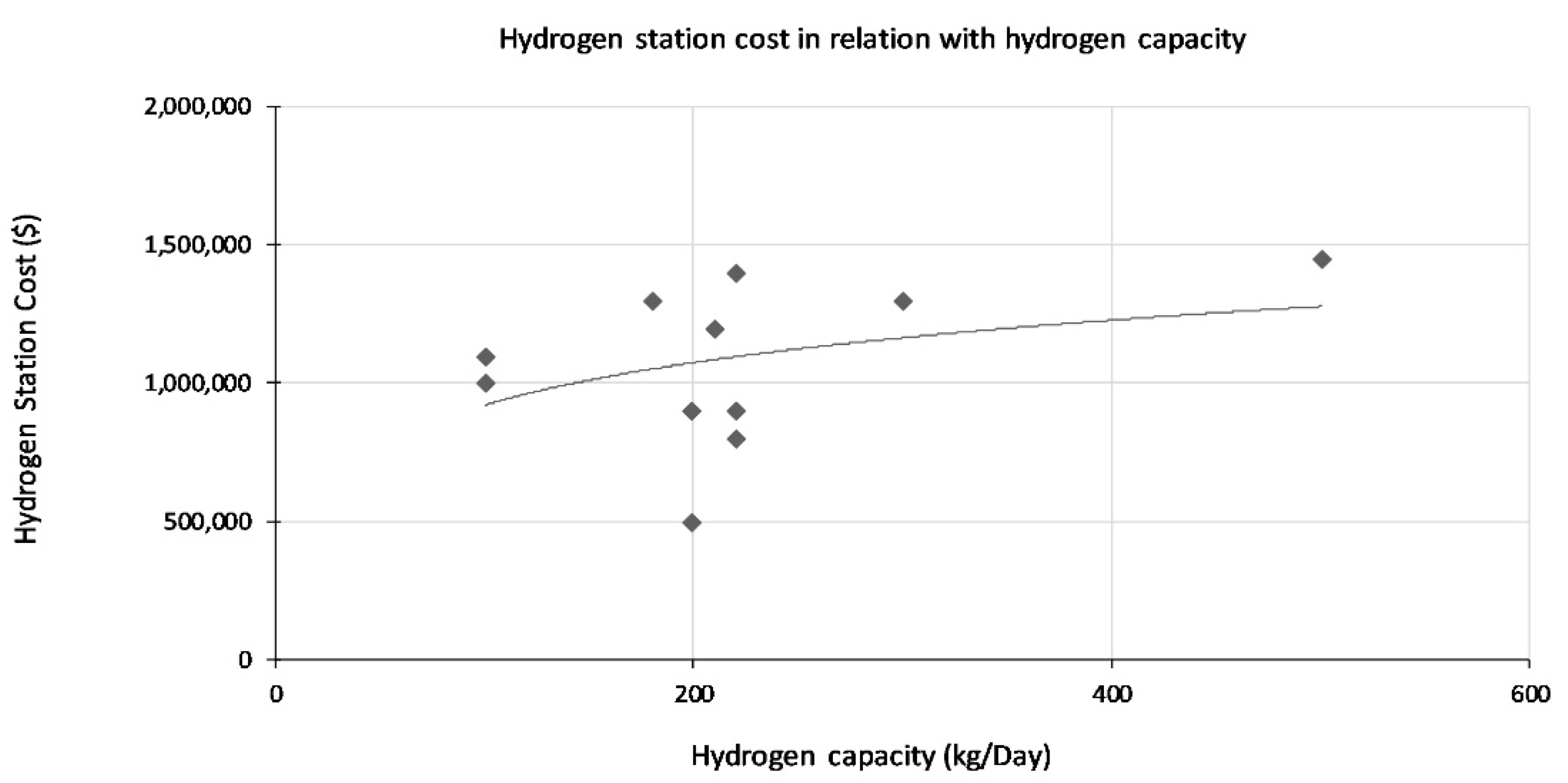
$/kg. Obviously, an increase in fuel demand affects the initial cost (see
Figure 5), but it has the opposite result to specific costs. Additionally, some basic parameters that can cause cost reduction are the H
2 market spread and technology evolution. Comparing this range of costs with the results of the current study, it can be concluded that the results are in good agreement with the results obtained by other researchers for most of the examined scenarios. The values of
Figure 5 has been derived from the study [
23].
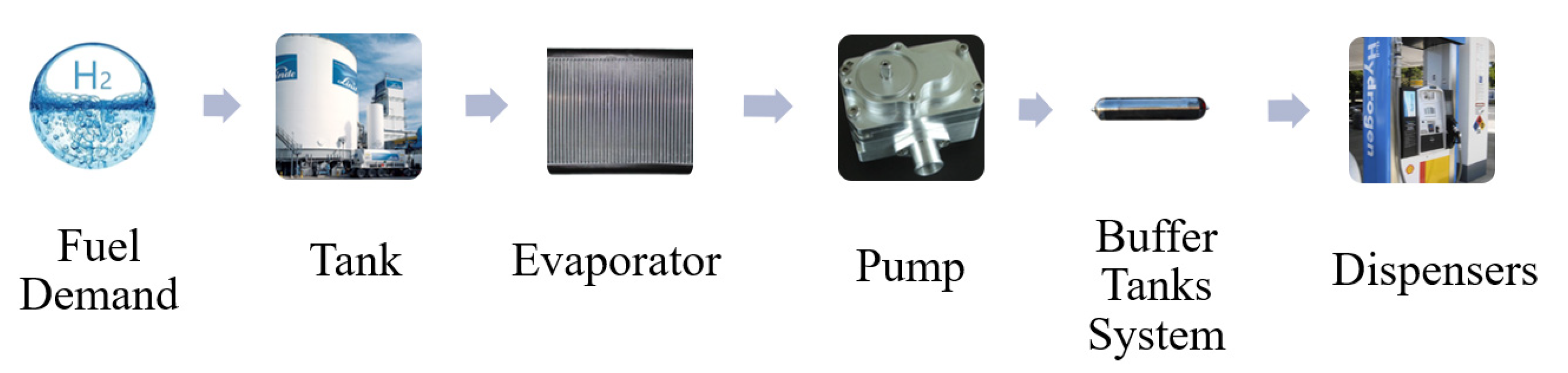
There are three HRS types: Gas-H
2 refills, the first HRS type, dispense (or store) 180 kg/day (average price), and the total cost of HRS construction is 2 M
$ (1.7 M€). The second type is the Liquid-H
2 (LH
2) delivery, and the differences in the equipment of HRS reduce the cost of the station. This kind of station can dispense 350 kg/day, but IC
o is higher than the first one (2.8 M
$). Nevertheless, the high capacity of HRS, with liquid-H
2, causes a significantly lower ratio of cost per kg of H
2. The most cost intensive kind of station is the HRS with onsite production of H
2. Capacity is limited, but the equipment is also more complicated and extraordinary (cost intensive). The capacity is only 120 kg/day, and the total cost equals 3.2 Μ
$ [
24].
Taking into consideration the above average values, a ratio of cost per kg can be calculated to compare with the results of this research. Especially, HRS with gas-H2 has a capacity equal to 65,700 kg annually (maximum). Based on cost and capacity, the specific cost is estimated at 14.42 €/kg. As for HRS, which stores LH2 in its tank, IC equals 2.38 M€ (2.8 M$), but its capacity is 350 kg/day or 127,750 kg/year. Consequently, the specific cost is significantly lower than gas-H2 (10.63 €/kg). The most cost intensive project is HRS with onsite production, as it is already mentioned. The tank of this station can refuel FCEV with 120 kg/day or 43,200 kg/year due to the production part, which restrains the required space. As a result, the specific cost equals 30.51 €/kg, which is considered very high. Nevertheless, it is an objective discussion to consider which type of HRS is optimal since many factors and indicators should be estimated and evaluated.
Comparing the above values with the last scenario (indicatively) of this research is compelling for determining the meaning of results and ensuring credibility, as it has the highest capacity (or demand). Based on the results of the sixth scenario, the annual fuel demand equals 16,900 kg/year (or annual H2 stored 26,600 kg/year), and the capital cost is ~€694,000 (no subsidy). Consequently, the specific cost of HRS is 12.8 €/kg for this occasion. In case there is a subsidy, the specific cost can be essentially reduced, and it would be equal to 11.5 €/kg with 50% subsidy. Compared with 10.6 €/kg of relative example with LH2 (above), there is an essential declination between the two values (without subsidy). However, it should be considered that this HRS was considered to be constructed in a remote region of Greece, which means that transfer of equipment would be cost intensive. In addition, low fuel demand is the main cause of this project’s low income, and the H2 production station was considered to be far from HRS, close to the wind park. Consequently, these factors affect the cost degree of HRS during its construction (and operation); therefore, there is a +14% burden. On the other hand, it is still an alluring investment compared to the average price of the three examples (above), which is 18.3 €/kg. Last but not least, the first project in an upcoming field is usually subsidized by a government and as a result possibility for profitability (viable investment) and motivation of an investor are considerable in a Greek remote region.
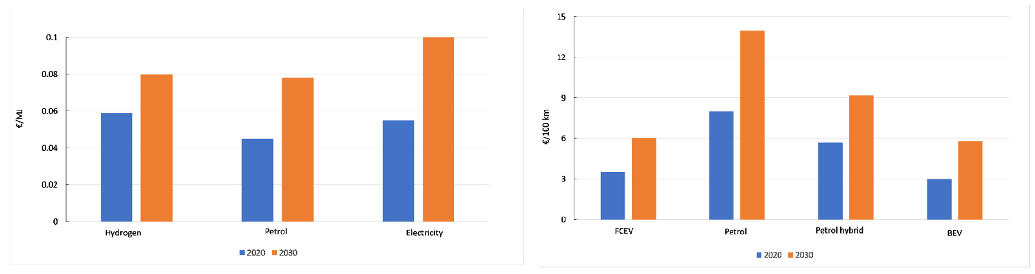
On the other hand, the cost for the vehicle owners is crucial for the spread of “green vehicles” in the market, as it indicates the ability of H
2 to compete with fossil fuels and motivates the market to purchase FCEV. Additionally, it is essential for the investment risk, which is high for investments in remote regions (in general). Based on the Shell H
2 study [
25], petrol vehicles seem to be the most cost intensive due to fuel efficiency. Especially, Battery Electrical Vehicles (BEV) cost the owner about ~6 € per 100 km in contrast with a conventional car, which demands approximately 9 € per 100 km. As for FCEV, they cost 6.1 € per 100 km (forecasting for 4.5 €/100 km). According to Kolb et al. [
26], diesel is the only fuel that approaches the cost of FCEV and BEV. Specifically, 6.3 € per 100 km are required for a diesel vehicle. Nevertheless, emissions indicate a decreasing usage of fossil fuels (mainly diesel). Additionally, their price is vulnerable to unexpectancies, i.e., wars, accidents, COVID-19, etc. Additionally, Shell hydrogen study [
25] states a future projection (2030) of fuel cost for vehicles, which indicates that declination between petrol vehicles and FCEV-EV will be increased by a factor of 2.5 times. That said, the cost for FCEV and EV owners will be equal (approximately), as FCEVs have a greater fuel range (see
Figure 6).
Figure 6 has been derived considering the data from the study [
25].
Considering the results of this research,
Table 4 indicates the fluctuation of cost per 100 km among six scenarios. Focusing on scenarios 3–6, which will have capital growth, fuel costs are ~7 €/100 km (average). There is a considerable decline (~13% burden) when the average value of these scenarios is compared with 6.1 €/100 km [
25]. Another parameter, which configures the weight of subsidization in the spread of H
2 in Greece, is the cost/100 km which indicates the advantage of H
2 compared to other conventional fossil fuels, especially in the remote rural regions. Even if the first discussion for HRS’s construction (LH
2) in a remote Greek region seems to be profitable at some point (petrol: 14.8 €/100 km), more aspects should be considered, such as cost for vehicle owners. Thus, the role of the Greek government (consider an economic crisis) is to finance HRS construction and acquisition of FCEV (or reduce cost by another method) to motivate investors and habitants of remote regions.
From an economic perspective, the cost/100 km constitutes a reliable parameter for determining which is the most economically viable solution. More precisely, the average cost for a remote user is 7 €/100 km approximately while the average world values are at 6.1 €/100 km, ensuring that H2 is a competitive fuel even if HRS locates in remote regions. Consequently, it can motivate the replacement of conventional vehicles, considering the cost of the fossil fuels for vehicles owners (9–14.5 €/100 km). Focusing on the investor’s cost, the energy cost of HRS (from a pump) is 0.25 €/kg vs. 0.23 €/kg (world average). Especially, the total cost for the investor (specific cost of HRS) equals 12.9 €/kg in a remote region, which is 19% higher than the world average cost (future projection: 6.2 €/kg). Thus, there is a considerable difference, mainly from the obstacles of a remote location, such as the equipment transportation in a distanced location. Additionally, the number of FCEVs is confined in a remote region compared to a city, which can cause low income for an HRS and a high cost of fuel.
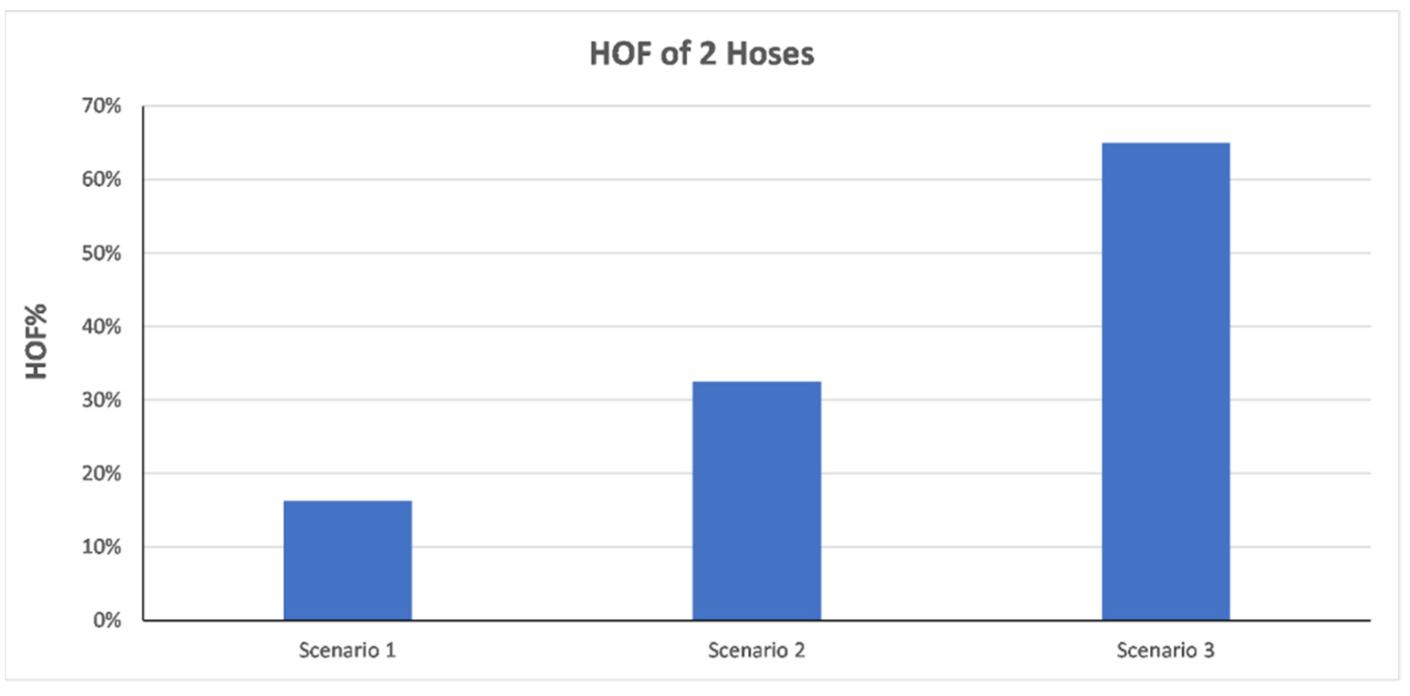
As for the sizing results, monthly demand determines the size of equipment. Consequently, the storage tank is the main component that can vary in each scenario to meet the refueling requirements. As previously mentioned, the storage tank is increased by 50% approximately when the number of FCEVs is doubled. In addition, the buffer tanks capacity between 25 and 100 FCEVs is about 18.8 kg. In the fourth scenario, a buffer tank with a capacity of around 37.6 kg is required, indicating that the size is doubled over 100 vehicles. For scenarios 5 and 6, the capacity is increased by about 25% compared with scenarios 3 and 4. The main tool for HRS sizing and evaluation of its operational efficiency is HOF. More precisely, the first case examined was with one dispenser for scenarios 1, 2, and 3. More specifically, in scenarios 1 and 2, HOF is 16% and 33%, respectively. In the third scenario, HOF equals 65%, indicating that two dispensers would be a proper solution for reducing the HOF index below or equal to 50%. However, economic indicators can significantly affect the final choice regarding the equipment that is applied. Overall, installing one dispenser seems to be the optimum solution for scenarios 1 and 2 (
Figure 7).
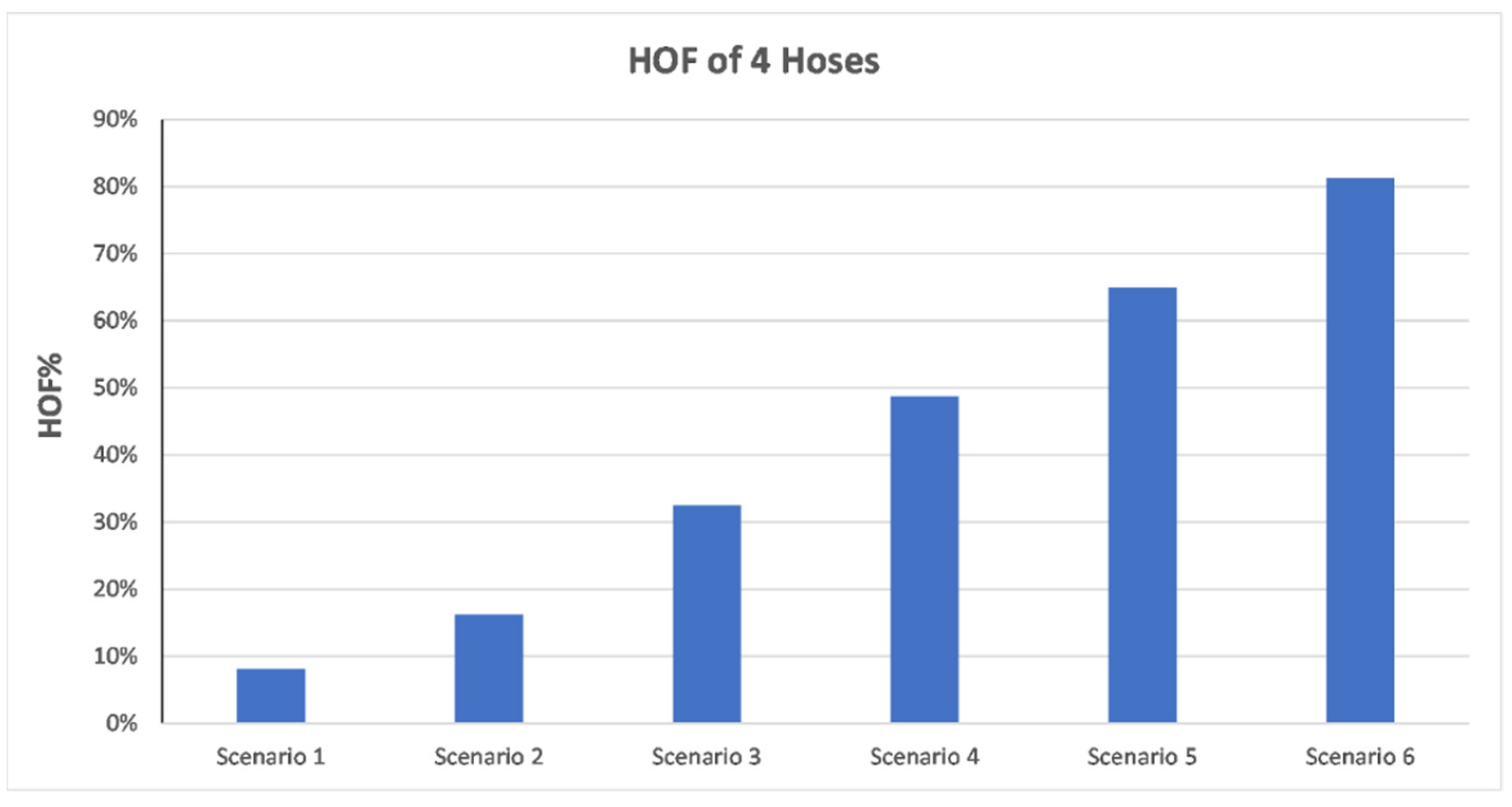
In
Figure 8, the case with two dispensers for all six scenarios was examined. Nonetheless, the application of two dispensers seems to be an oversized solution for scenarios 1 and 2 since HOF is about 8% and 16%, respectively. In addition, scenario 3 presented an improvement reaching HOF around 30%, while scenario 4 presents HOF at 49%. Moreover, scenarios 5 and 6 present HOF at 65% and 81%, indicating that more dispensers are required.
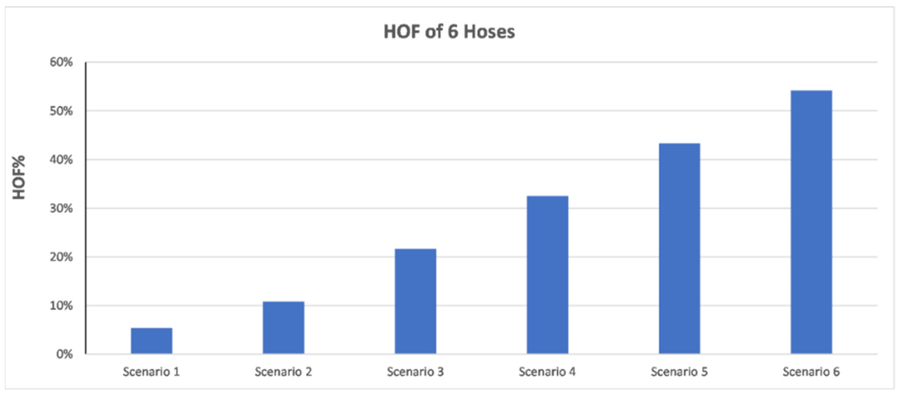
In
Figure 9, three dispensers for all six scenarios were examined, and it is concluded that the system in scenarios 1, 2, and 3 have been oversized. However, a significant improvement is noted in scenarios 4 and 5, reducing the HOF index from 49% to 33% and from 65% to 43%. However, scenario 6 presents a high HOF index indicating that a solution with four dispensers could be more appropriate.
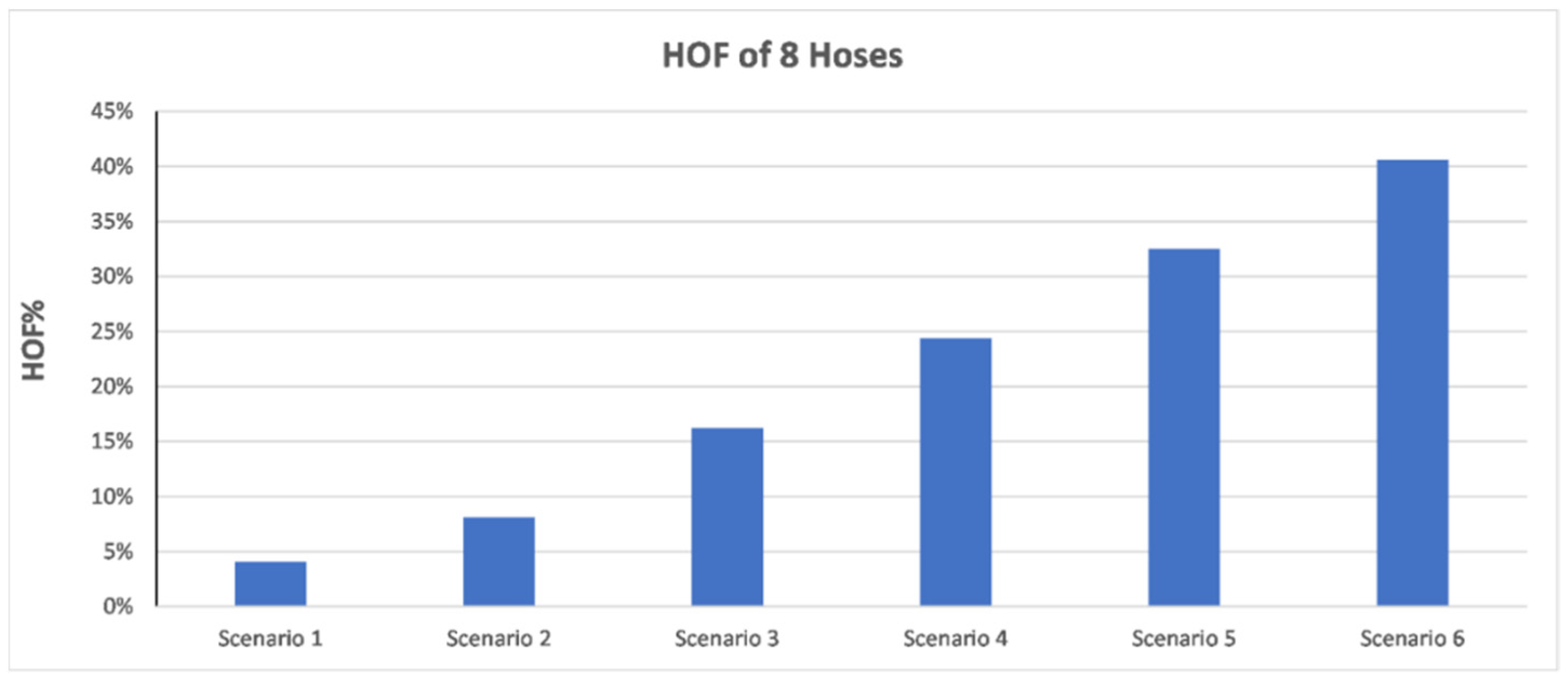
Finally, four dispensers for all six scenarios were examined. From
Figure 10, it is concluded that the HOF index has been within legitimate limits. Thus, this solution can be characterized as economically viable since the specific cost has not increased significantly. Nevertheless, in scenario 6, the HOF index was reduced to 41%. However, as mentioned previously, this scenario could be economically viable in developing regions with higher FCEV penetration.
The cryopumps are the most cost intensive part of the equipment reaching almost 32% of the total invested capital. Thus, due to the low number of FCEVs in remote regions, one pump is suggested. In this respect, the optimum tank capacity in relation to the number of vehicles that will be refueled can be determined. It should be considered that vessels can be found in the market in standard specific volumes, usually resulting in an oversized tank. Moreover, the number of dispensers is a crucial selection because this component balances the service time of FCEV, the cost of the equipment, and the forecasting for the fuel demand on a life cycle basis. The main criterion for this decision is the HOF, which should remain lower than 50%. However, this study focuses on remote regions where an increase in fuel demand seems to be impossible based on population and market capabilities.
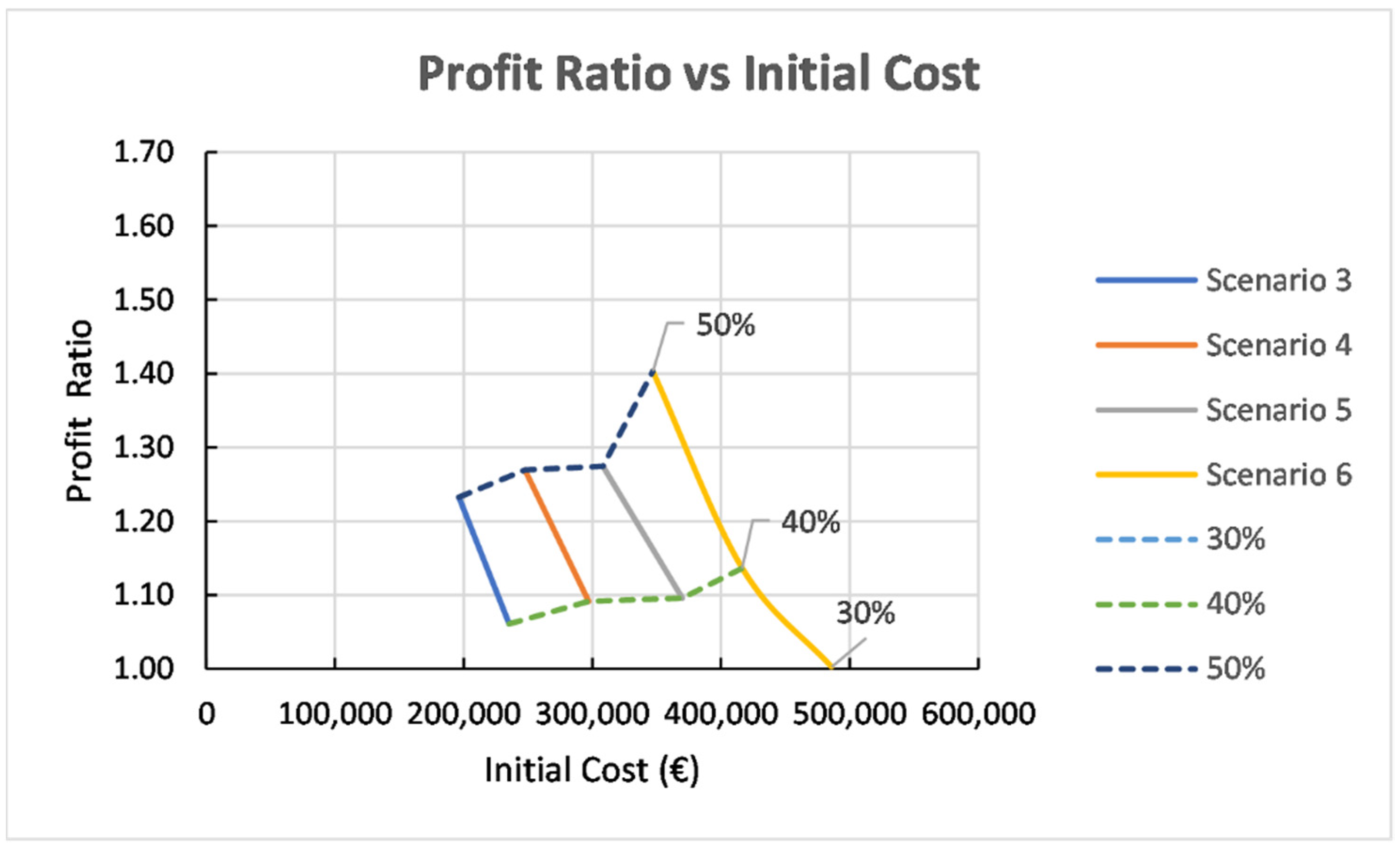
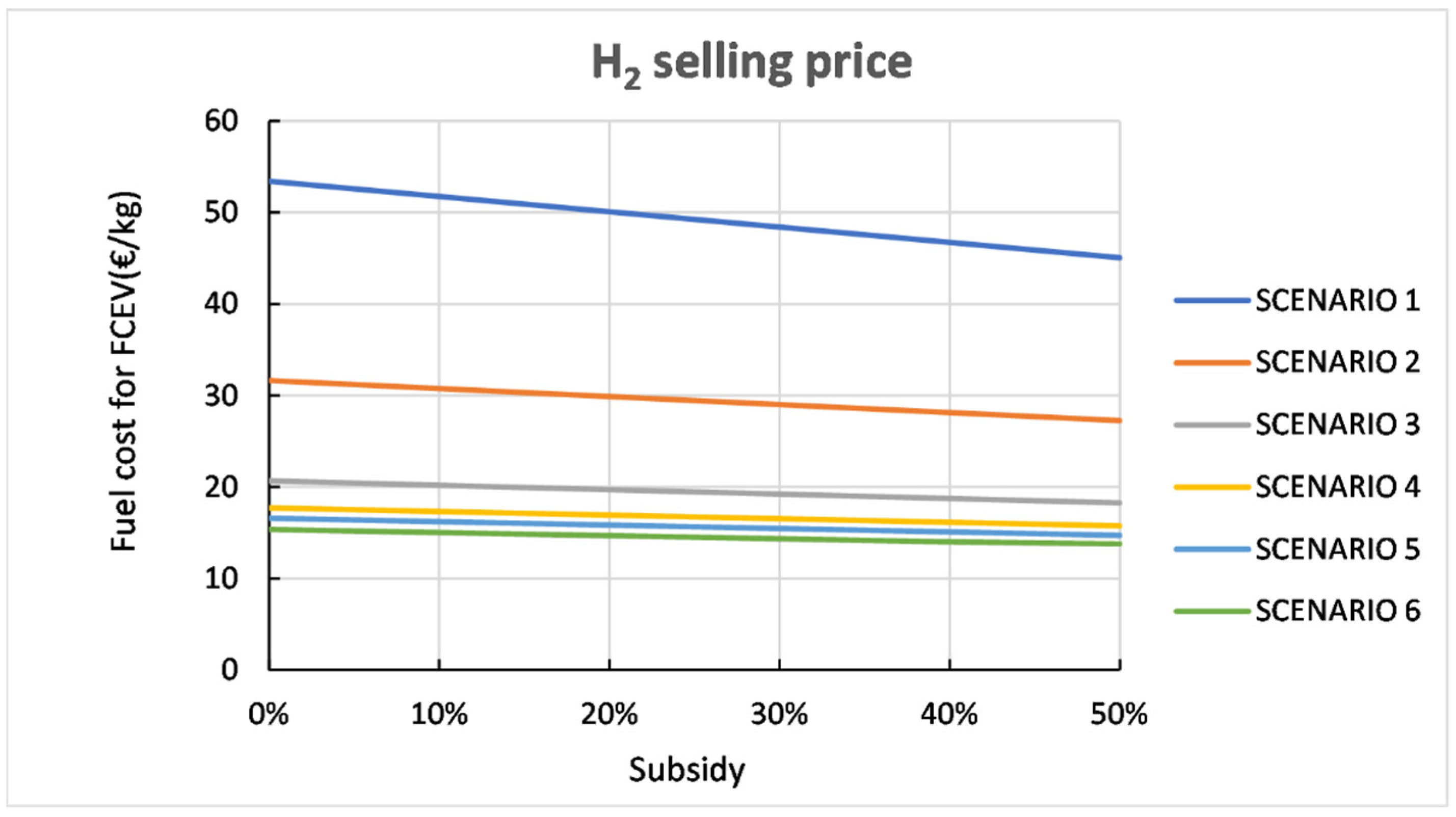
The cost of fuel, the selling price, and the corresponding payback period, IRR, and profit ratio for all six different scenarios considering various subsidy values were also investigated. By taking into consideration
Figure 11, it is concluded that increasing the demand reduces the cost of H
2. This implies that the size of the equipment applied in the HRS can affect the corresponding revenues. One thing that should also be considered is that, as the subsidy increases, the cost of H
2 decreases, highlighting that novel technologies should be supported.
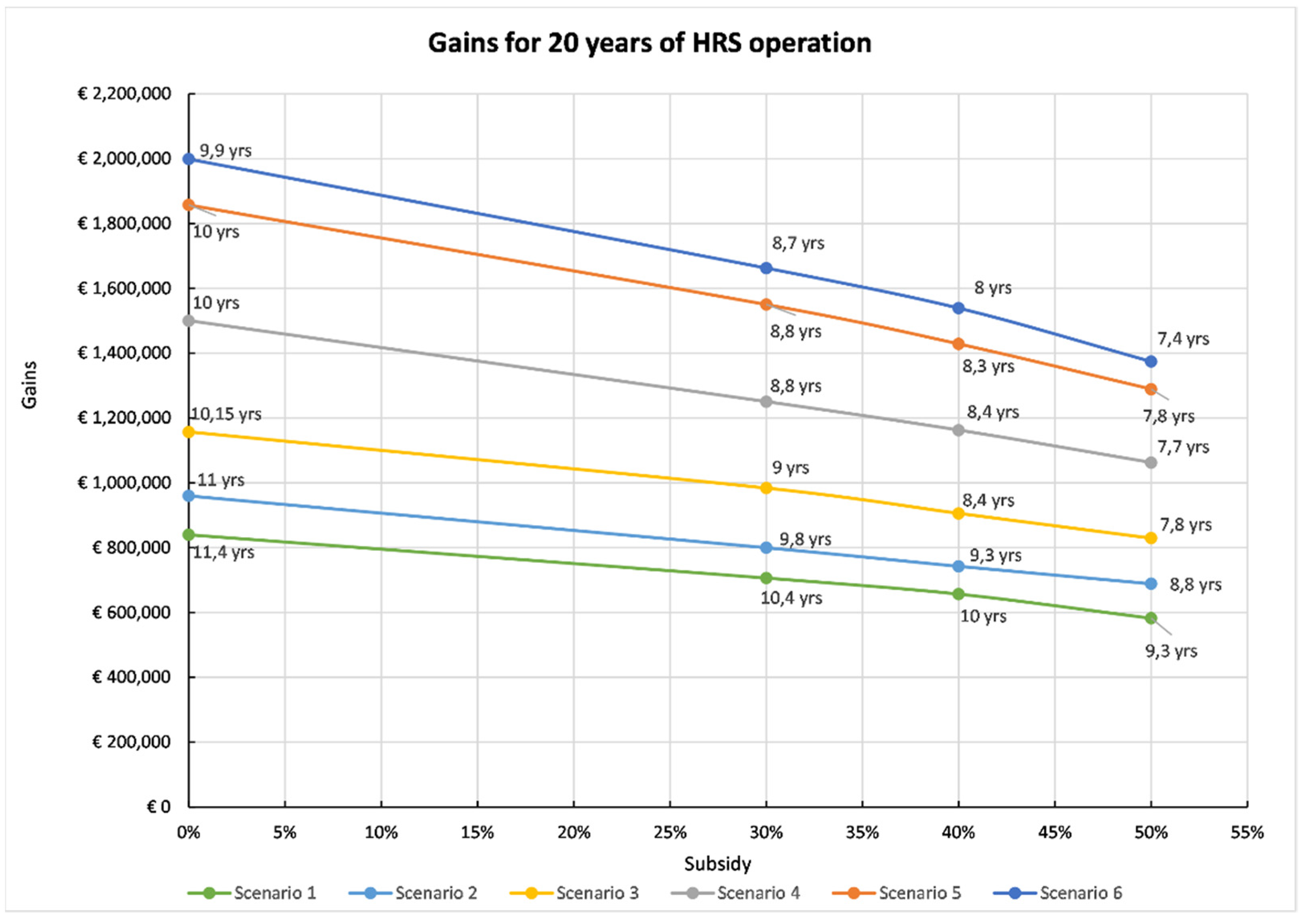
The analysis of initial cost, maintenance and operation costs, and the revenues on 20 years base can ensure the possibilities for the profitability of each scenario. However, it should be considered that the long-term evaluation can have significant deviations, which depend on the assumptions, reliability of data, and unexpected changes in the economy (market) and technology. Thus, a comparison between costs and revenues is beneficial (
Figure 12) in which the payback period is indicated with bullets.
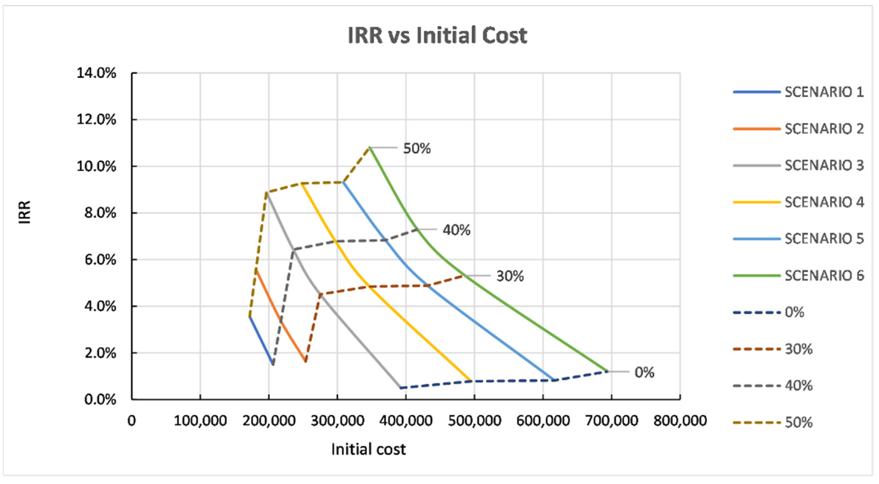
In scenario 1, the payback period ranges between 9.3 and 11.4 years (approximately), while the subsidy significantly affects the repayment of invested capital. In scenario 2, higher revenues are presented, and the payback period ranges from 8.8 to 11 years. Additionally, the economic support by the government has a vital role in minimizing the payback period. In scenario 3, the payback period is about 10.2 years without subsidy. Despite that, the payback period can be reduced to 7.8 years, with a subsidy at 50% approximately, motivating the investor for the specific scenario. Similar results are presented in scenario 4, while in scenarios 5 and 6, revenues are significantly increased compared to the third and fourth scenarios. Further evaluation should be conducted considering the values of IRR and PR for providing more accurate results. Scenario 1 presents low IRR and profit ratio values, indicating that the specific solution is not economically viable even if the subsidy reaches 50%, as presented in
Figure 13 and
Figure 14. Furthermore, similar results are obtained for scenario 2, although it presents slightly improved economic performance.
On the other hand, scenario 3 is the first one to be considered as a profitable one. However, at least a 35–40% subsidy is required to increase the initial value of the investment. In scenario 3, there is 6% capital growth when the subsidy reaches 40% (IRR = 6.4%). On the other hand, with a 50% subsidy, the growth increases by 2%. In addition, the profit ratio takes values above 1, indicating the economic viability of the specific scheme (
Figure 13). In the fourth scenario, a growth of the invested capital is presented compared with the third scenario, starting when the subsidy reaches 40%. Specifically, there is a 27% increase in PR value in conjunction with IRR (50% subsidize), which equals 9.3%, while the PR presents higher values than scenario 3. In scenario 5, there are slight differences in comparison with scenarios 3 and 4; thus, it can be considered as equal. Finally, in scenario 6, significant outcomes are presented considering a subsidy of 30% or less, presenting a maximum PR value around 1.40, indicating that the specific solution is the most economically viable.
As for the future of investments in remote regions, estimations could only be made. Because this technology is becoming more efficient (year by year) in all parts of its life cycle, the cost has significant possibilities to be reduced. Additionally, the spread and the evolution of other technologies affect the cost of H2. For example, more and more wind turbines are installed with high efficiency in many remote regions. This study also proves that the burden is the initial cost of the investment and, under appropriate conditions/arrangements, can be affordable (economic efficiency and penetration in the market).


