Abstract
Energy consumption in buildings is expected to increase by 40% over the next 20 years. Electricity remains the largest source of energy used by buildings, and the demand for it is growing. Building energy improvement strategies is needed to mitigate the impact of growing energy demand. Introducing a smart energy management system in buildings is an ambitious yet increasingly achievable goal that is gaining momentum across geographic regions and corporate markets in the world due to its potential in saving energy costs consumed by the buildings. This paper presents a Smart Building Energy Management system (SBEMS), which is connected to a bidirectional power network. The smart building has both thermal and electrical power loops. Renewable energy from wind and photo-voltaic, battery storage system, auxiliary boiler, a fuel cell-based combined heat and power system, heat sharing from neighboring buildings, and heat storage tank are among the main components of the smart building. A constraint optimization model has been developed for the proposed SBEMS and the state-of-the-art real coded genetic algorithm is used to solve the optimization problem. The main characteristics of the proposed SBEMS are emphasized through eight simulation cases, taking into account the various configurations of the smart building components. In addition, EV charging is also scheduled and the outcomes are compared to the unscheduled mode of charging which shows that scheduling of Electric Vehicle charging further enhances the cost-effectiveness of smart building operation.
1. Introduction
The worldwide electrical energy consumption of the building sector which includes both residential and commercial buildings is about 20% of the total energy produced [1]. The building sector alone is responsible for 35% of greenhouse gas emission, 65% of halo-carbon and approximately 30% of black carbon emissions [2]. Due to the rapid growth in population and fast economic growth, building energy consumption is expected to rise at a pace of 1.3% per year from 2018 to 2050 [3]. The detrimental environmental impact of this rising energy consumption has sparked widespread concern throughout the world. Therefore, it is very important to improve the energy efficiency in buildings in order to reduce the carbon emission and mitigate carbon footprint. For these reasons, buildings nowadays are required to be both energy efficient and environmentally friendly, with renewable energy being used in part or entirely instead of fossil energy, notably solar energy. Integration of passive solar systems in buildings is one option for sustainable growth in this direction. Annual heating demand can be reduced by up to 20% using passive solar approaches [4]. Several architectural elements, such as solar roofs [5], solar chimneys [6], Trombe walls [7], etc., are mostly employed in today’s construction of buildings. Trombe walls, also known as storage walls or solar heating walls, are a popular choice among these devices due to their ease of installation, high efficiency, and low operating costs [7]. Apart from being ecologically benign, putting a Trombe wall in a building may save up to 30% overall energy consumption. [8].
The rapid increase in global electrical energy demand and its generation from conventional resources, along with the increasing integration of intermittent and inexhaustible renewable energy resources to the electricity network called for enhancement and updating of the existing electrical grid infrastructure to obtain efficient, reliable, and clean energy [9]. Consequently, this emerges the concept of the smart grid from which the consumer can intelligently manage their energy consumption [10]. It is feasible to construct a two-way energy exchange system using Micro-Grids (MGs). MGs will not only be utilised for peak shaving, load shifting, and energy management, but will also strive to optimise RES integration in order to reduce power exchange with the main grid. [11]. When more than one energy source is used to fulfill a certain load, an efficient energy management system is required [12]. The construction of an Efficient and Intelligent Building Energy Management systems (BEMS) with the objective of minimizing energy cost by the integration of Fuel Cell, RES, EVs, BESS, and Heat Storage Tank is indeed a challenging task.
In this paper, a certain number of distributed energy resources (DER) components are connected to a large scale residential building connected to a bidirectional utility grid is considered. These components consist of a photo voltaic and wind turbine installation, a fuel cell based CHP system, a battery storage system (BSS), and a number of EVs used for day to day work-related trips. Stochastic characteristics are used to model the mobility behavior of EVs used in this study. A bi-directional energy flow mechanism is considered for the energy produced by the DERs between the grid and smart building. In this research work, the smart building energy management system (SBEMS) has been designed to optimize the energy consumption and building automation by utilizing the energy management system (EMS). SBEMS fulfills all the objectives of energy savings, centralized control of the system, decreased human resources, enhanced human security, and finally reduced human error. The major goal of utilizing SBEMS in buildings is to profit from the economic benefits and optimum control of energy consumption, as well as to provide a safe and peaceful environment. The SBEMS system can easily be accessed from anywhere, both outside and inside the building, by using appropriate software via internet and mobile communication.
1.1. Literature Review
The concept of a smart building (SB) is a novel issue in recent study, and it has a lot of potential for development due to its varied nature. Though SB appears to be highly appealing, it confronts a number of problems, particularly those related to energy management [13,14]. Numerous studies have been carried out to address issues and development of smart building energy management system (SBEMS), and the following is a detailed review of the available literature:
The author in [15] develops a mathematical model for building energy management that is compromised of a BSS, a PV, and a plug-in EV. Using a rule-based controller, the model in this study manages the power flow between the resources. The Author in [16] developed a new hybrid genetic-based harmony search (HGHS) approach for modelling the home energy management system, which helps to reduce consumers’ electricity bills and usage during peak load hours by scheduling both household appliances and smart home deployed energy resources during peak load hours. In Ref. [17], a Home Energy Management (HEM) system with small-scale renewable energy generation and BSS is being investigated. The model is built on a mixed-integer linear programming formulation that takes vehicle-to-grid (V2G) and demand response techniques into account. To better guide peak shaving techniques, researchers investigated the best energy management of a building energy system (BES) using multi-energy flexibility metrics, especially under the energy payback effect. It was discovered that load recovery is an unavoidable aspect of the demand side management (DSM) process, and that ignoring it might result in overestimating the response value and potentially have a detrimental impact on DSM goal outcomes [18]. The author in [19] presents a strategy for reducing a building’s power usage and electricity expenditures by optimizing the charging and discharging of Plug-In Hybrid Electric Vehicles (PHEVs). The main goal in the research work [20] is to minimize the daily electricity charges. Moreover, energy generated from PV and building load demand is forecasted using a stochastic model. In order to optimize the operation cost of a micro grid, the BSS scheduling optimization is presented in [21] on a micro grid application level. The deployed model’s restrictions include energy balance and power limitations for both EVs and BSS. Furthermore, binary variables are utilized to ensure that storage batteries are not both charged and drained at the same time. In Ref. [22], a mixed-integer linear programming model for EV charging is suggested, taking into account the use of PV production.
A review of EV charging techniques is presented in [23,24]. Charging techniques are broadly classified according to: un-regulated charging, off-peak hours charging, and charging to reduce peak demand and increase load factor. It has been noticed that the first two approaches are simple to execute but provide little value when compared to the last two techniques, whereas better voltage values and an improved frequency profile is achieved in the third and fourth techniques along with enhanced integration of renewable energy resources and also the load profile is flattened. In [25], the effects of EV charging on power system voltage are evaluated, and a strategy to mitigate the impacts of EV loading is presented.
The intermittent characteristics of renewable energy resources (RES), as well as the stochastic nature of EV departure and arrival timings, provide a challenge to the power grid. However, experts are researching ways to improve their combined operation both technically and economically [26,27]. In [28], a fast charging station is optimally designed for an EV integrated with BEES and renewable energy resources by using genetic algorithms and Monte Carlo techniques. For the combined operation of electric vehicle and renewable energy resources, an adaptive and robust optimization technique is suggested in [29], which considers the uncertainties in the time-in and time-out of EV.
When EV is used with micro-CHP, it generally results in better economy in comparison to when they are operated individually as reported by many authors [30,31,32,33]. A case study [30] was carried out in Italy, in which two semi-detached residential buildings are considered in two different sites and their combined operation is compared with their individual operation, and it is reported that up to 60% of cost saving is achieved in combined operation. The author in [31] developed a combined model of EV and micro-CHP and evaluated the system using an MILP technique, and the author found that the combined operation of both results in better efficiency.
The previous work contributes significantly to literature and provide a platform for future study, whereas the integrated behavior of RES, CHP, battery, EV, neighborhood heat exchange, and heat storage tank in a bidirectional electricity grid necessitates further observation as the present economic and environmental problems address for their combined use at the smart building. The aforementioned research work does not address the optimized scheduling and integrated operation of thermal and electrical demand of smart buildings [23,25,34,35,36,37,38,39,40,41,42,43,44,45,46]. Likewise, the rising trend of EV adaptability and its charging effects on power system needs significant attention because the EVs consist of a major part of the electrical demand in a modern smart building.
1.2. Contribution and Paper Organization
The research paper is organized and presented in the following manner:
- First of all, the smart building model is developed which includes a fuel cell based CHP system, heat storage tank, neighborhood heat exchange, electrical vehicles (EV), battery, PV, and wind turbine. Bidirectional utility is considered for this case flat and variable type of tariff is used for analysis.
- Optimization model of smart building is developed for the cost-effective working of Smart Building Energy Management System (SBEMS). Constraints for the system and device are carefully selected and well defined. A real coded genetic algorithm (RCGA) is utilized to solve the problem of building demand response and optimal scheduling of its resources.
- Eight different test cases are developed, based on different scenarios, in order to fully analyze and explore the role of different components installed in the smart building. The results obtained from these different cases revealed the fascinating attributes of the optimization process and the smart building energy management model.
The rest of the article is organized into: Section 2 specifically introduces the development of the smart building model and its different items. Section 3 explores the technique used for the optimization problem and their constraints related to SB’s load and components. Section 4 elaborates the use of RCGA and its implementation in the smart building model. Section 5 discusses simulation and results of test cases. Finally, Section 6 presents the conclusion and future work recommendations.
2. Development of the SB Model
The Smart Building considered in this study is a multi-story residential building having 100 residential apartments. Normal electric and thermal load have been considered for every individual apartment. In addition, a Plug-in Electric Vehicle (PEV) which acts as a load while in charging mode is considered for each apartment. The necessary building related details are given in Table 1. The schematics of a proposed modern SB model are given in Figure 1. The SB thermal and electrical demand is fulfilled from different types of power resources such as electric power and natural gas. The power flow is divided into two loops:

Table 1.
System parameters.
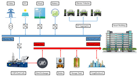
Figure 1.
Overview of a smart building.
Electrical Loop
It is composed of responsive and non-responsive electrical resources and demands (i.e., utility, Fuel Cell, RES, and BSS). Electricity from utilities, fuel cell, battery, and renewable energy resources powers the domestic appliances and charges the electric vehicle batteries. This study considers the two-way flow between utility companies and SB. Therefore, when power is needed, SB buys power from the utility and sends the excess power to the utility.
Thermal Loop
It is composed of heating load, boiler, heat obtained from fuel cell, heat exchange between the community, and heat storage tank. Natural gas is used to power fuel cells and auxiliary boilers. The heat energy wasted from fuel cell is obtained and is used to meet the building heating demand. If the heat obtained from fuel cell is inadequate to fulfill the overall demand of thermal energy, then auxiliary boiler, neighborhood heat exchange, and storage tank is used to provide the insufficient heat energy.
2.1. Modeling the Fuel Cell
Fuel cells are available in different sizes and shapes based on the fuel type used and their design. The different components of a typical FC are shown in Figure 2. A power conditioning unit, fuel processing unit, and a stack are all important parts of the fuel cell. This research study considered an FC based on proton exchange membrane operated on natural gas while providing heat and electrical powers as outputs.
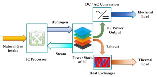
Figure 2.
Fuel cell based CHP model.
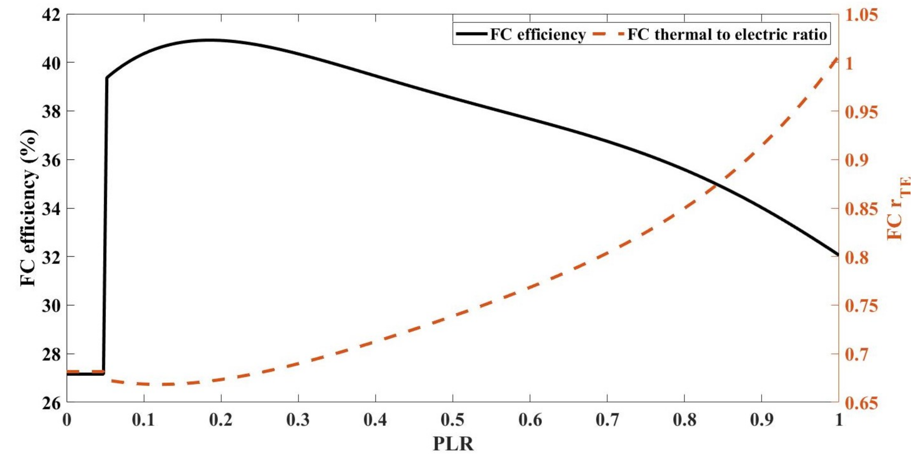
Part load ratio (PLR) is used to calculate the efficiency of fuel cell. The PLR is the ratio of electrical power obtained from a fuel cell at the i-th interval to its maximum power ratings, as calculated by Equation (1):
where is the PLR at the i-th interval for the output power of FC () during this interval.
Mathematically, the efficiency of fuel cell and thermal to electrical power ratio of FC () for the i-th interval is given below [47]:
When :
When :
Now, the thermal power generated by fuel cell at time interval i is measured as:
The relationship among FC efficiency and PLR is represented in Figure 3. It is evident from the curve that the FC’s performance is poor at low PLR because of large parasitic losses [47], whereas, after this low PLR area, the fuel cell operates at 30–40% efficiency. It is clear from the efficiency curve that the values of are relatively large at lower PLR regions as compared to peak power of FC’s usage.
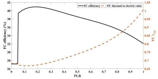
Figure 3.
Role of PLR on and of Fuel Cell.
2.2. Electric Vehicle Modeling
Modeling of electric vehicle relies on many factors, like deriving style, type of route, distance traveled by EV and state of charge at plug out time. In this paper, the area of study is focused on residential building, which is why we considered an electric vehicle for each apartment of the smart building. Four different types of EVs are selected from a list of top 10 EV models by sale in the USA [48]. Nissan Leaf [49], Chevy Volt [50], Kia Soul [51], and Tesla Model 3 [52] are selected for the analysis purposes. The different parameters of the four selected electric vehicles are given in Table 2. In this study, it is considered that all the participants’ EVs complete their battery charging when they leave the building in the morning. As the time interval () is taken as 60 min, the available slots in a particular day is therefore 24. AC level type 2 is taken as an EV charging device in this study.
Table 2.
Specification of EV models.
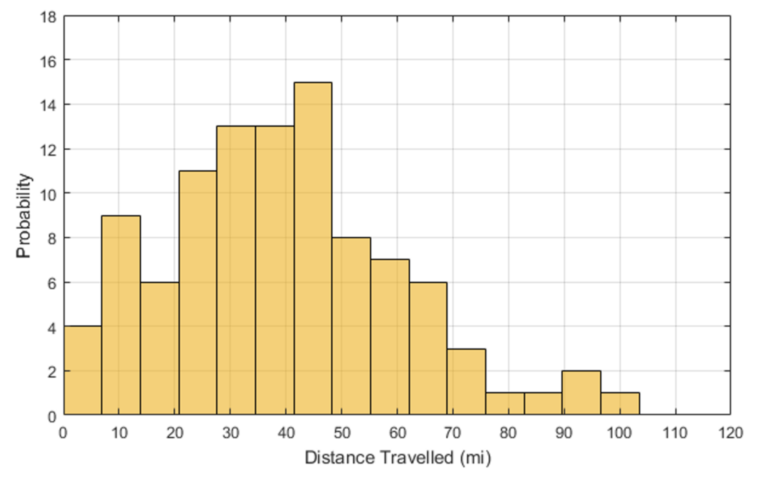
Required travel data of EVs such as time of arrival, time of departure, and daily distance traveled are randomly generated based on statistical probability by using data obtained from [53]. Random data sets for the arrival time and departure time are generated through normal distribution. To randomly generate EVs’ departure times from the building, the value of and are taken to randomly generate the departure time from the building and for the arrival time at the building the value of and are considered. Log-normal distribution with and is used to randomly generate the values for the daily traveled distance by EVs [54]. Matlab probability distribution function is used to calculate time of departure, time of arrival, and distance traveled per day are represented in Figure 4 and Figure 5.
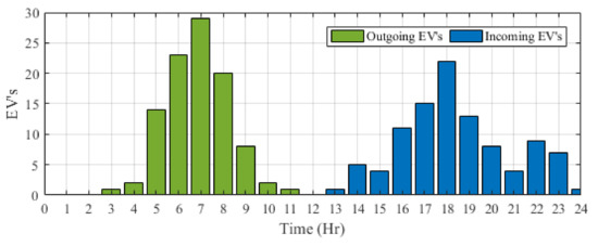
Figure 4.
Probability of EVs’ time in and time out.

Figure 5.
EVs’ daily distance traveled.
This research work considers SOC (state of charge) at plugged in-time depends on the distance traveled per day and used the data available in [55]:
where
Charging power (kW)
SOC of EV (%) at interval i
Plugged-IN SOC of EV
Plugged-OUT SOC of EV
Minimum SOC of EV(%)
d Daily travelled distance (km)
Net drive efficiency (km/kWh) of EV
EV battery capacity (kWh)
If the values of d and are available, then is determined by using Equation (7). It is clear from this equation that, in order to safeguard the EV batteries, a lower boundary condition is applied to .
Equation (8) schedules the charging process of EVs:
2.3. Modeling the Battery Storage System (BSS)
The battery storage system model is presented in Equation (9), which governs the process of charging and discharging of batteries:
where is the energy of the battery at the i-th interval, and denotes a power column vector that holds the battery charging and discharging powers, whereas is the charging efficiency and is the discharging efficiency. T is the simulation step time. When the battery is charging (), the valve of is taken as positive (+ve) and, when the battery is discharging (), the value of is taken as a negative value. It is also worth noting that the vector will only store one value (either positive or negative) at any given time interval and the other value will be placed at zero.
2.3.1. Modeling the Neighborhood Heat Exchange
The availability of the Neighborhood Smart Building (NSB) for buying from and selling to the SB is modeled as:
where and are the maximum buying and selling limits of the NSB, and is the availability of NSB for either heat buying from or selling to the SB at interval i. Note that +ve value of means that NSB has surplus heat to offer to the SB while negative values shows that it itself needs thermal energy.
2.3.2. Modeling the Heat Storage Tank
The storing of thermal energy to the HST is governed by Equation (11):
The discharging of thermal energy from the HST is governed by Equation (12):
Here, is -ve during heat storage and +ve when heat is removed from the HST.
2.4. Electricity Tariffs
Here, in this research paper, a ’peak valley tariff’ is used for selling (export) and for buying (import) of electricity from the utility [56,57]. The peak valley tariff is widely used across the globe as it offers different unit prices at different time intervals during the day for the electricity consumption. Another advantage of using a peak valley tariff is that it reduces the stress on the utility grid and also helps in improving the overall load factor of the utility grid. The peak valley tariff used in this study has three different blocks (valley, plain, and peak) used in their respective time as mentioned in Table 3. It is evident from Table 3 that the buying price () is higher then the selling price () of peak valley tariff in order to give benefit and attraction to the buyer to purchase electricity from a smart building.
Table 3.
Peak valley tariff.
2.5. Renewable Energy Generation
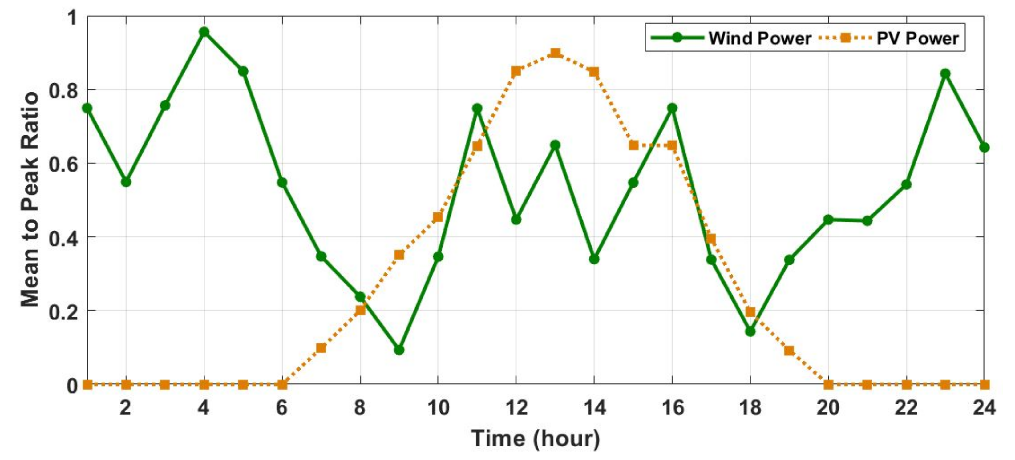
In this research, PV system and wind system are used as renewable energy resources. A typical power curve [58] PV and wind are shown in Figure 6. As we know, the power produced from wind and the PV system depends on weather conditions. During the day time (9:00 a.m.–5:00 p.m.), in the presence of sunlight, the PV produces its maximum generation while the wind power fluctuates sharply, whereas, during the night, the wind power produces its peak and PV stop working because of the unavailability of solar irradiance. It should be noted that both curves for wind and PV power are forecasted (estimated) and the mean-to-peak ratio value of wind power is 53.6% and PV power is 26.46%.

Figure 6.
PV and wind profile.
3. Optimization Model
This section introduces an optimization model of SBEMS for the proposed SB model. The primary objective of SBEM is the optimization of energy produced and utilization of various resources and demands to minimize the total system cost while fulfilling its constraints. Therefore, the objective of this research work is the minimization of daily energy cost of SB.
3.1. Objective Function
The objective function is the minimization of 24 h energy cost of the smart building, as given in (13):
where
n No of hours
T Span of time interval (h)
Startup cost of FC ($)
Shutdown costs of FC ($)
FC total cost ($)
Total cost Boiler ($)
Total cost of Utility ($)
Cost of battery at interval i ($)
Natural gas purchasing cost ($/kW)
Utility buying cost ($/kW)
Utility Selling cost ($/kW)
Battery operation and maintenance cost ($/kW)
Electrical output of FC at time i (kW)
Boiler heat generation at time i (kW)
Utility power at time i (kW).
Energy buying price of utility ($)
Energy selling price of utility ($)
FC efficiency
For purchasing the power from utility, the value of will be positive, and, for selling the power to utility, the value of will be negative.
3.2. Constraints
In this section, the constraints related to the power balance and devices installed in the smart building are explained and presented in the following subsections.
3.2.1. Power Balance Constraints
Electrical Power Balance Constraint
In order to avoid load shedding, the SBEMS should fulfill the electrical demand completely.
During the charging of battery, the power balance equation will be:
In addition, during the discharging of battery, the power balance equation will be:
where
Electrical load at interval i
Wind power at interval i
PV powers at i-th interval
BSS charging or discharging power at the i-th interval .
EV charging power at i-th interval
Charging efficiency of the BSS
Discharging efficiency of the BSS
During the charging interval of BSS, is negative, and, during the discharging interval, it is positive.
Thermal Power Balance Constraint
The heat requirement is fulfilled from FC, boiler, neighborhood heat exchange, and heat storage tank. Therefore, three different strategies are used for thermal power balance. The constraints related to each strategy are explained as under:
Strategy 1: Heat from FC and Boiler
where is the output of the boiler in at interval i.
Strategy 2: Neighborhood Heat Sharing
If heat is sold to the Neighborhood Smart Building:
If heat is bought from the Neighborhood Smart Building:
Strategy 3: Heat Storage Tank (HST)
When heat is stored in the HST:
If heat is sold to the Neighborhood Smart Building:
If heat is bought from the Neighborhood Smart Building:
when heat is removed from the HST:
If heat is sold to the Neighborhood Smart Building:
If heat is bought from the Neighborhood Smart Building:
3.2.2. Device Constraints
The smart building devices’ constraints are presented as below.
Fuel Cell Constraints
The rate of change in the fuel cell’s output power is subjected to the ramp rate constraints for smooth functioning of fuel cell:
Similarly, the FC output is controlled by the power generation’s minimum and maximum constraints:
where
Ramp Up rate of FC
Ramp down rates of FC
Minimum power of FC
Maximum power of FC
Electric Vehicle Constraints
In order to prevent any damages to the EV battery, its max charging and state of charge (SOC) limit must be taken into consideration:
where Maximum limit of EV charging power
Maximum limit of SOC of the EV battery
BSS Constraints
The following are the maximum energy and minimum energy constraints of the battery that must be fulfilled:
When the BSS is charging:
When the BSS is discharging:
where
BSS energy level at Time i-(kWh)
BSS energy lower limits
BSS energy upper limits
Maximum charging rates of battery
Maximum discharging rate of battery
Neighborhood Smart Building Thermal Constraints
If is the excessive or required thermal power at the NSB side at interval i, then it must fulfill the following maximum selling and buying constraints.
If NSB is buying thermal energy from the SB:
If NSB is selling thermal energy to the SB:
Constraints of Pipes Connecting the Buildings
A thermal efficiency of the pipes connecting the neighboring buildings is considered. The heat loss during the heat transfer intervals between the buildings will be taken care of by the building which is selling heat. Therefore:
If SB is buying from the NSB ( NSB is selling), then:
However if the SB is selling to the NSB ( NSB is buying), then:
Heat Storage Tank Constraints
The minimum energy and maximum energy constraints of heat storage tank that must be fulfilled are as follows:
During heat storing:
During heat releasing:
4. Real Coded Genetic Algorithm
Modern heuristic techniques are fast and emerging tools for optimizing nonlinear systems. They are generally superior to traditional derivative-based techniques, which have the limitations of trapping into local minima, computational complexity, or in-applicability to certain objective functions. The genetic algorithm (GA) is one of the most widely used evolutionary algorithms in power system applications. Its mechanism is based on the evolution of nature, and the algorithm essentially consists of genetic selection, hybridization, and mutation operations applied to chromosome populations. RCGA is an enhanced version of GA and is used for optimization in this research. For numerical optimization problems with real values, the integer or floating point representation of global variables in RCGA is better than the binary representation of variables in GA. Compared with GA, RCGA provides higher consistency, higher accuracy, and faster convergence speed [59].
RCGA is an efficient method, and the optimal solution can be found without deriving the objective function. Therefore, unlike linear programming or derivative-based techniques, RCGA can effectively deal with various objective functions and constraints, whether they are smooth or non-uniform; linear, nonlinear; continuous, discontinuous; convex, and non-uniform convex. Comprehensive details of RCGA are given in [60,61,62]. The following sections provide an overview of the processes involved in this method, which employ RCGA to model and solve the SBEMS optimization problem:
4.1. Step I: Initialization
The first stage of RCGA, like other global optimization approaches, is to construct the starting population. Chromosomes are the name for the first population. The chromosomes are made up of genes, each of which reflects the power (kW) of a certain device in the SB. If N represents the overall genes in a chromosome, then the location of i-th gene is illustrated by:
The SBEMS’ dimensionality must be taken into consideration. There are dependent and independent variables in the system given in this paper. The RCGA uses the independent variables for optimization. Here the independent variables are , , and . Dependent variables , , , , , etc. are calculated from fixed variables of power demands and resources. Lastly, these variables are utilized in Equations (14)–(19) to determine the overall cost of energy.
The cost of the SB is calculated by the RCGA during a 24-h period. This study employed a one-hour time period. As a result, the SBEMS is investigated for 24 time sections and four variables (, , , ) in each time slot determining the size of optimization problem .
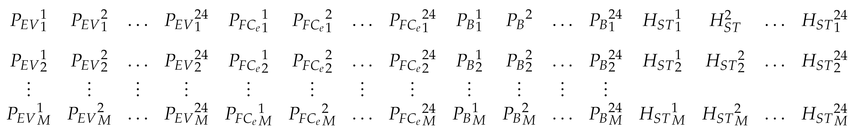
If M is the number of chromosomes in one generation then gives the dimensionality in terms of one generation of the RCGA as shown in Figure 7.
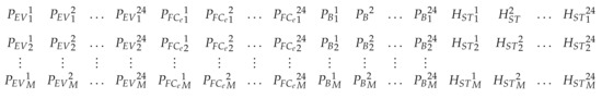
Figure 7.
Chromosomes in one generation of the RCGA.
4.2. Step 2: Implementation of the Constraints
During each time interval, the system constraints for and are checked. Section contains the equations that control this stage are given at Section 3.2.2. The flow chart in Figure 8 shows the logical process and variable operations in the RCGA for satisfying these requirements.
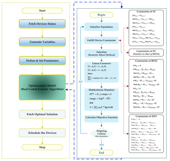
Figure 8.
Proposed SBEM flow chart.
4.3. Step 3: Using RCGA Operators
4.3.1. Selection
In the RCGA, one of the most important processes is the selection of the fittest person for each consecutive generation. Individuals (chromosomes) are chosen with care for future generations depending on their fitness value. Some frequent selection procedures include ranking, tournament, and roulette-wheel. The roulette-wheel selection technique is used in this work to carry out the selection operation [63].
4.3.2. Crossover
The search space must be reached by the starting population for the RCGA to effectively search for the potential solution. A crossover operation is performed to assure the GA’s global search feature. In RCGAs, this operator is quite important. In actuality, it is considered as its distinguishing feature [64]. It should be noted that this operator does not apply to all chromosomes throughout the process of establishing intermediate populations. The crossover rate, also called as the crossover probability, is used to quantify the likelihood of crossover application on a chromosomal pair [65].
4.3.3. Mutation
The mutation operator alters one or even more genes on a specific chromosome at random to increase the population’s basic variability. RCGA can prematurely converge to sub-optimal solutions if it is not subjected to mutation. This operator’s job is to reintroduce undiscovered or lost but viable solutions into the population’s search space. The RCGA method has a non-zero probability of arriving at any solution in the search space thanks to mutation. Every chromosomal location in the population has an arbitrary probability of suffering a random change. This phenomenon is expound by mutation probability, or mutation rate . Muhlenbeins Mutation operator presented in [66] is applied here.
With crossover and mutation, another selection strategy, called elitism is used to ensure that the finest chromosomes always remain uninjured from one population to the next [67].
The flowchart shown in Figure 8 depicts the different steps involved in implementing RCGA to optimize scheduling of the Smart Building Energy Management System (SBEMS).
5. Simulation Results
In this section, different simulation scenarios are presented which demonstrate the significant characteristics of the suggested optimization model of the smart building energy management system. The renewable energy resources, fuel cell, battery storage system, peak valley tariff, electric vehicle scheduling, and heat sharing between Neighborhood Building and Heat Storage Tank are included incrementally into the SBEMS as given in Table 4.
Table 4.
Proposed test cases.
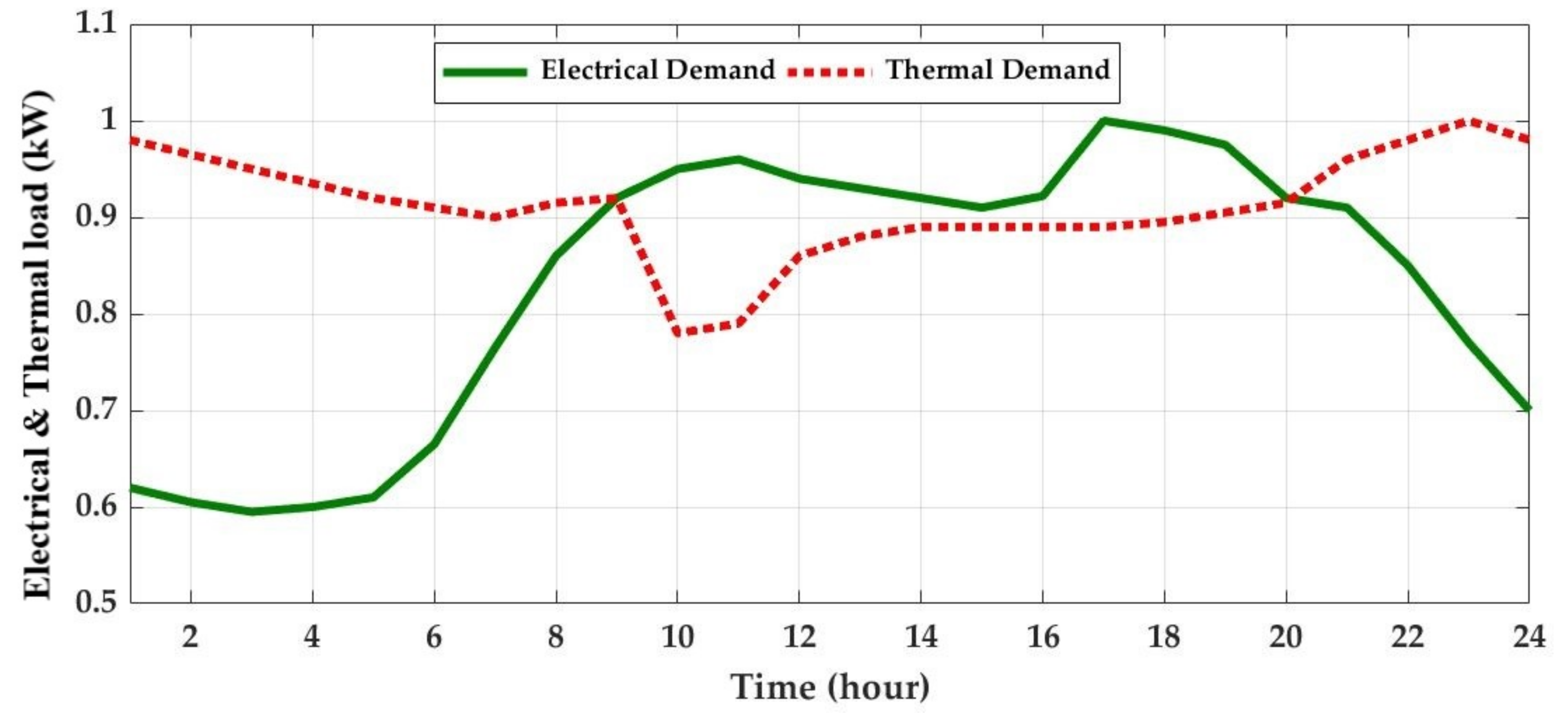
Figure 9 represents the normalized thermal and electrical load demands of a modern smart building [68]. The maximum thermal demand is taken as 50 kW, while the maximum electrical demand is taken as 200 kW. Table 1 summarized the values of different variables used in this study.

Figure 9.
Daily electrical and thermal load requirements of a smart building.
5.1. Base Case
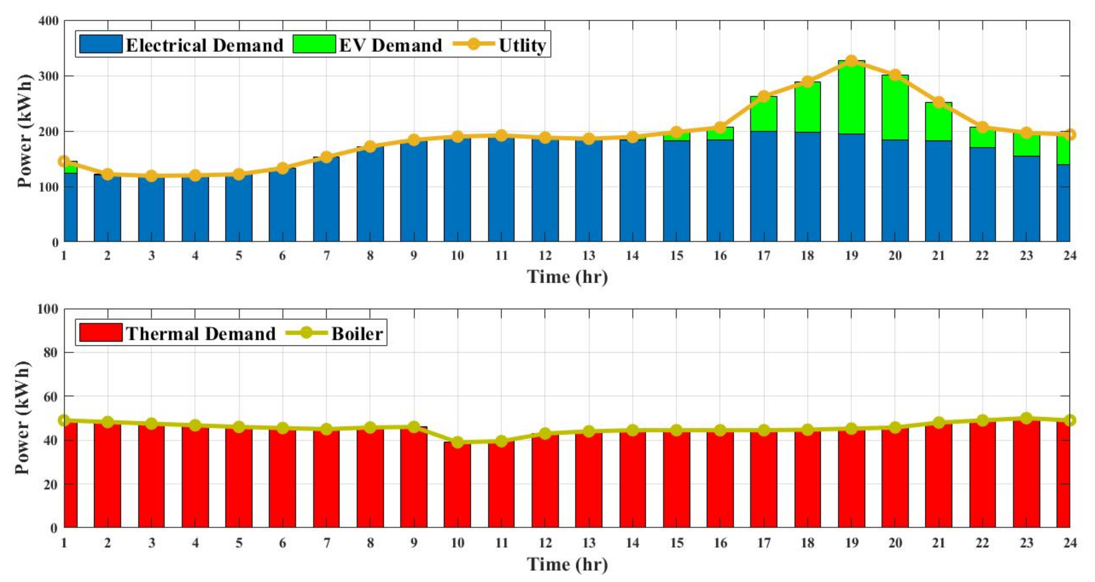
In this case, the smart building electrical demand is fulfilled by the utility and the thermal demand is fulfilled by the boiler which uses natural gas as shown in Figure 10. Unscheduled EV charging is adopted in this case; as soon as the EV arrived at the building, it starts charging. In this case, RES, BSS FC, scheduling of EVs, peak valley tariff, neighborhood sharing, and heat storage tank are not considered as shown in Table 4. The proposed optimization technique is not applicable in this case. This case will serve as a reference case for all other cases in this study. The net daily energy cost for this case is 658.95 ($/day).

Figure 10.
Base Case mode of house.
5.2. Case 1: Addition of Solar and Wind Resources
In this case, the impact of adding the solar and wind based RES to the smart building is analyzed. The solar and wind power resources have given priority in meeting the electrical demand of the building compared to the utility. While the heating demand of the building is fulfilled by using an auxiliary boiler. Utility is made bidirectional, so that the surplus amount of energy can be sold to the utility grid. Figure 11 represents the impact of adding solar and wind power to the building. Positive power indicates that power is purchased from the utility, while negative power indicated that surplus power sold back to the utility. In the intervals of 01:00–02:00, 03:00–06:00, 11:00–12:00, 13:00–14:00 and 16:00–17:00, the electrical demand of the building is less than the total RES generation, and the SB is selling excessive energy to the utility. The peak loading in the system occurs in 02:00–03:00, 06:00–11:00, 14:00–16:00 and 17:00–24:00 when the RES cannot fulfill the demand; therefore, the power is purchased from the utility. The net daily energy expenses for this case are $240.60, which is 63.48% lower than the base case.
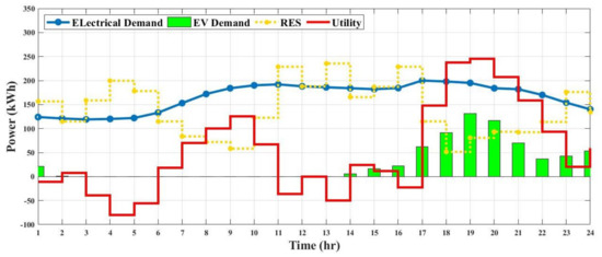
Figure 11.
Addition of renewable energy resources (RES).
5.3. Case 2: Addition of Fuel Cell Based CHP
In this case, a fuel cell base combined heat and power system is added to the smart building. The building thermal requirements are fulfilled by heat generated by FC and the boiler, whereas electrical demand is fulfilled by FC generated electrical power, RES, and a bi-directional utility.
As is evident from Figure 12 that the building electrical demand exceeded RES power at 7:00 a.m. and, from this time, FC initiates its operation to fulfill the increase load requirement. Most of the time, the building electrical demand is fulfilled from the the power generated from RES and fuel cell and the surplus amount of power is sold to the utility during time intervals 01:00–02:00, 03:00–06:00, 11:00–12:00, 13:00–14:00 and 16:00–17:00. Whereas, during time intervals 07:00–11:00 and 17:00–23:00, the combined generation of both FC and RES is insufficient to fulfill the building demand because of EV charging load from 5:00 p.m.–11:00 p.m. Therefore, the deficient power is purchased from the utility during these hours. The total daily energy cost of SB in this case is 212.44 $, which is 67.76% less as compared to the base case and 11.70% less than the previous case.
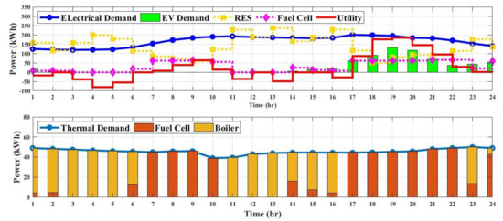
Figure 12.
Hybrid energy supply with the FC.
5.4. Case 3: Addition of Battery
In this case, the battery storage system is connected to the smart building and its impact is analyzed. It is worth noted that using utility and BSS together can only bring economic operation if and only if the product of BSS charging efficiency and discharging efficiency is greater than the valley-to-peak ratio. Due to this reason, BSS is charged during the valley region and discharged during peak hours. Therefore, it is important to introduce battery efficiency in this section, which is . In this research work, battery efficiency () is taken as 0.9, and the BSS charging and discharging pattern is shown in Figure 13. It is evident from Figure 13 that introducing a battery into the system results in economic operation. The daily operation cost of the smart building in this case is 203.30 $, which is 69.14% lower than the base case and 4.30% less than the previous case.
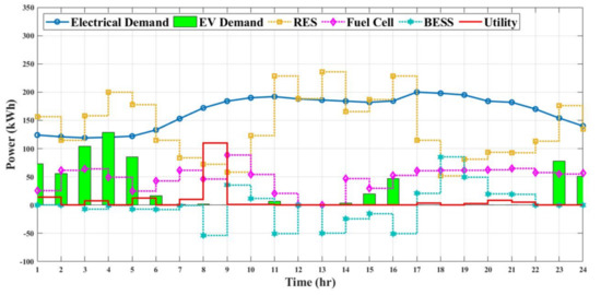
Figure 13.
Optimized generation schedule with BSS included.
5.5. Case 4: Introducing Peak Valley Tariff
Flat rate tariff is considered in all the previous cases in purchasing electricity from the utility. In this case, and the following cases, peak valley tariff is considered which is widely used in the present power market. The selling and buying rate of peak valley tariff are shown in Table 2. It is clear from Figure 14 that FC adjusts its output and BSS adjusts its charging in such a manner to take full advantage of the valley prices.
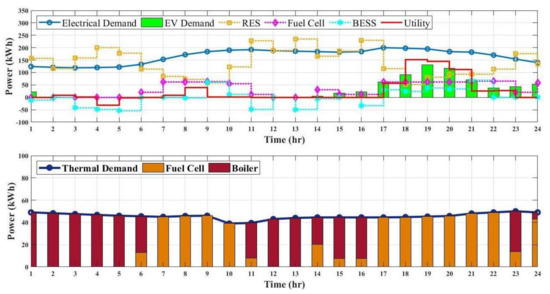
Figure 14.
Introduction of the peak valley tariff.
In order to obtain an economic operation in this case, the FC increases its output during peak hours and reduces its output during off-peak hours. Similarly, the BSS discharges during peak hours and starts charging during off-peak hours. This is because the optimization algorithm tries to get the minimum possible energy from the utility in order to achieve a nearly zero energy building concept. Due to the introduction of a variable tariff into the system, the net daily cost of the building reduces to 202.77 $, which is 69.22% less than the basic case and 0.25% less than the previous case.
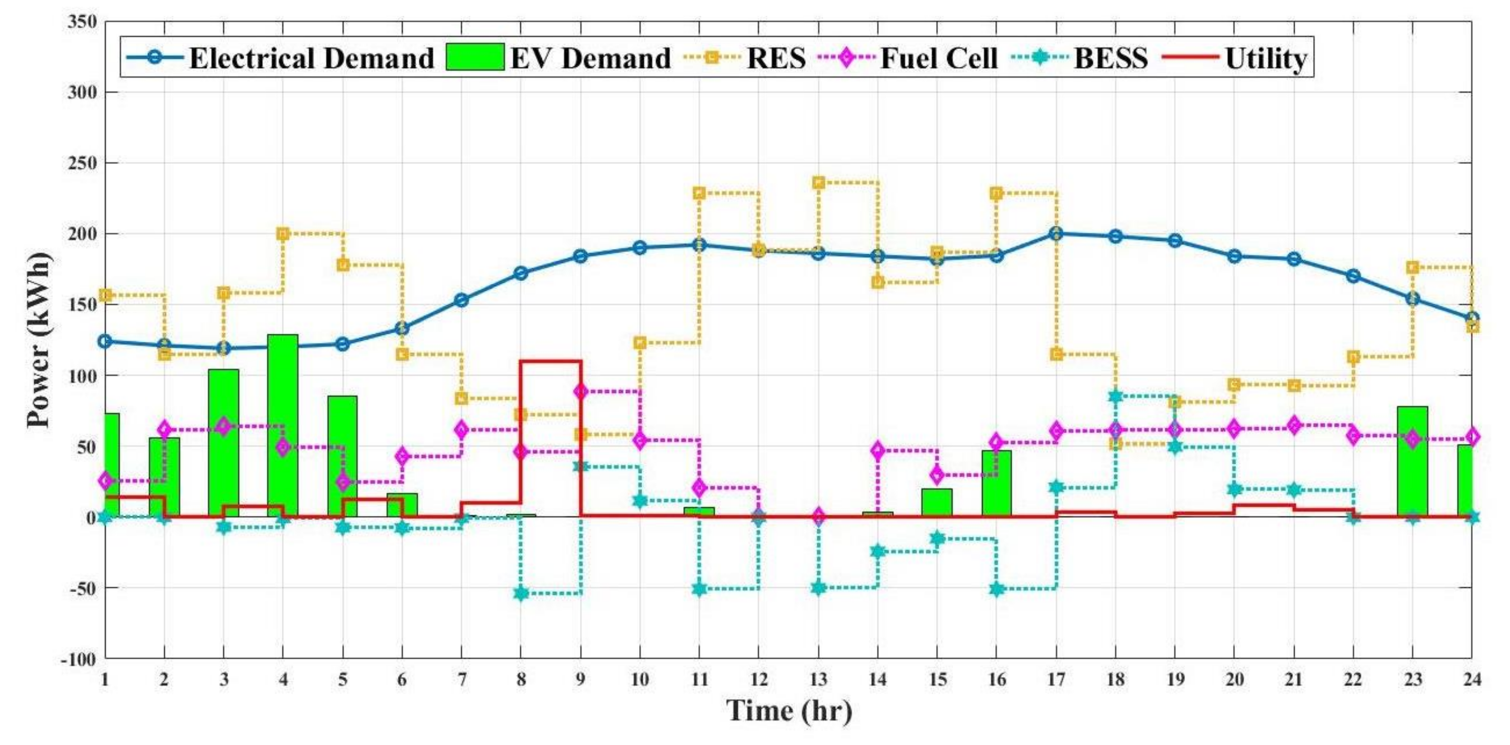
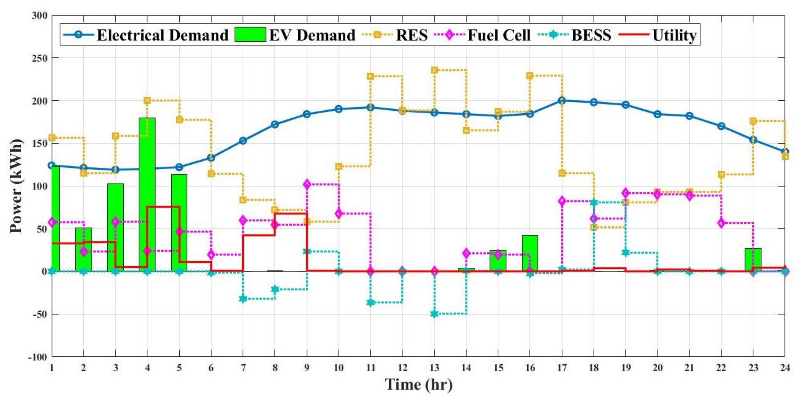
5.6. Case 5: EV Charging Scheduling
In this case, the electric vehicle charging scheduling is introduced into the system. As it is evident from the literature, scheduling the high power and non-critical electric load such as EVs, washing machine, etc. results in reducing the overall cost and improving technical benefits [44,45]. Figure 15 represents the scheduling of electric vehicle charging. The EV arrival time is shown in Figure 4. The EV is connected to the system as soon as it arrives at the building. However, the optimization algorithm schedules the charging of EV in those particular hours where consumers can get more benefits and reduces the overall cost of electricity. In this case, the net cost is reduced to 183.88 ($/day), which is 72.09% less than the base case and 9.31% less than the previous case.

Figure 15.
Results of the system with scheduling of EV.
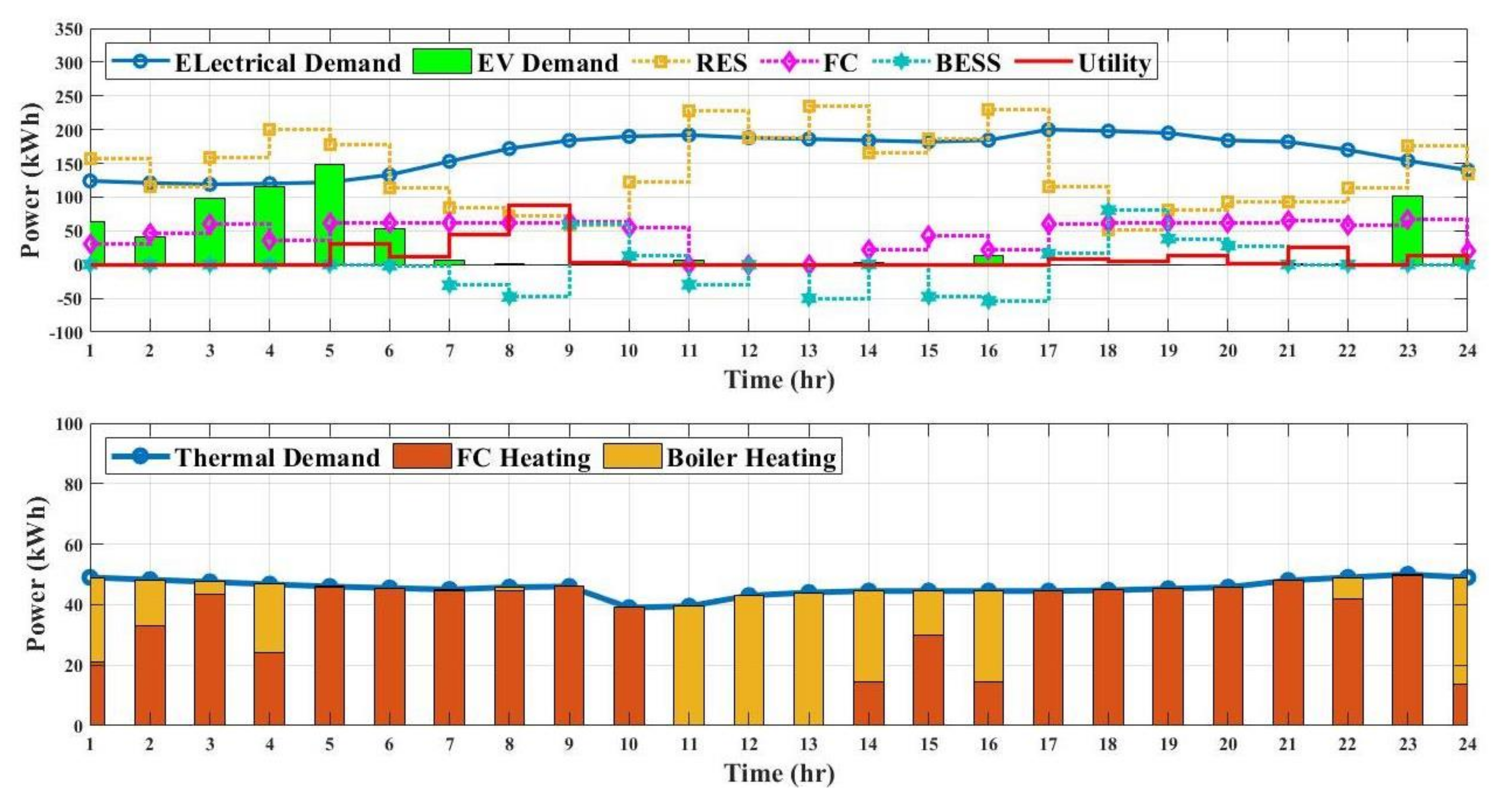
5.7. Case 6: Neighborhood Heat Sharing
In this case, a novel concept of buying and selling thermal energy from the neighborhood smart buildings is proposed. Figure 16 gives the electrical and Figure 17 depicts the thermal powers of the SB in this case.

Figure 16.
Electrical powers for Case 6.
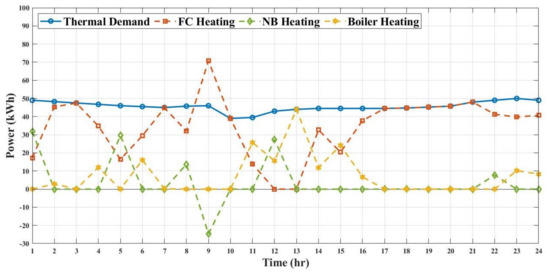
Figure 17.
Thermal powers for Case 6.
From 01:00–02:00, 04:00–06:00, 07:00–08:00, 11:00–13:00, and 21:00–23:00, the thermal demand is more than the FC thermal output and heat provided by the boiler. During these time intervals, the deficient heat is purchased from neighborhood smart buildings (NSB), and the SBEMS buys as much heat from the NSB as possible. The auxiliary boiler (AB) output is complementary to the heat availability from the NSB. For those hours, where NSB can provide more heat, AB output is comparatively less and vice versa. An interesting situation occurs at 04:00–06:00 and 11:00–13:00 hours. Here, FC can fulfill the SB’s thermal needs if it keeps on generating the same energy as it has been continuously providing. However, the SBEMS anticipated the heat availability from the NSB. It bought heat from the NSB and lowered the FC output, thus allowing FC to run on an improved efficiency. From 8:00 a.m. to 10:00 a.m., the heat generated from FC is more than the heat demand, so, during this period, the excess heat is sold out to the neighborhood smart building. For electrical loads of the SB, the utility output complements the FC and RES output. When FC and RES output is insufficient to fulfill the building requirements, then the utility provides the electrical energy in those hours. When electrical output from the RES and FC increases, buying from the utility decreases. The net daily cost in this strategy has reduced to 180.80 $, which is 72.56% less than the base case and 4.09% less than the previous case.
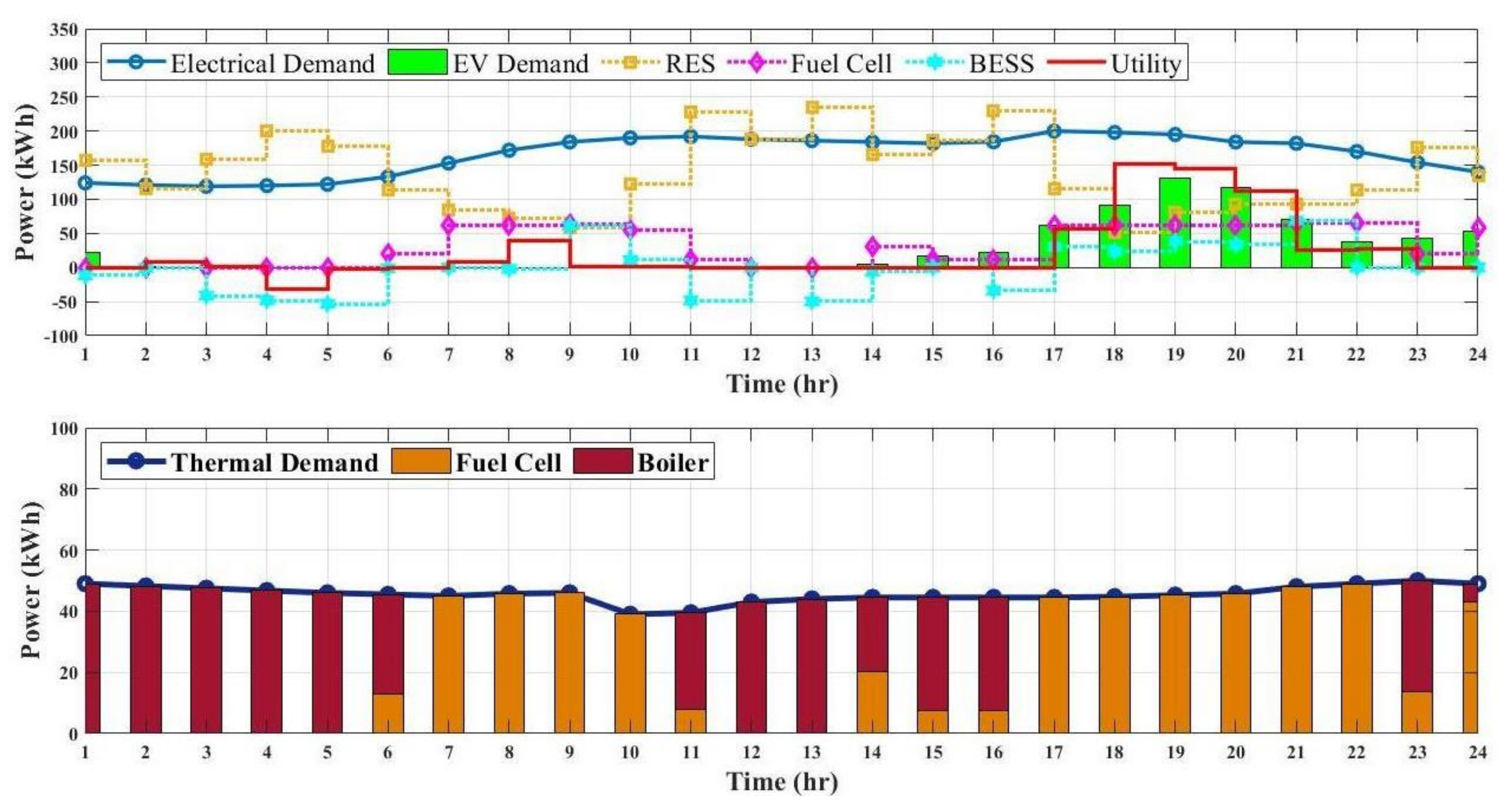
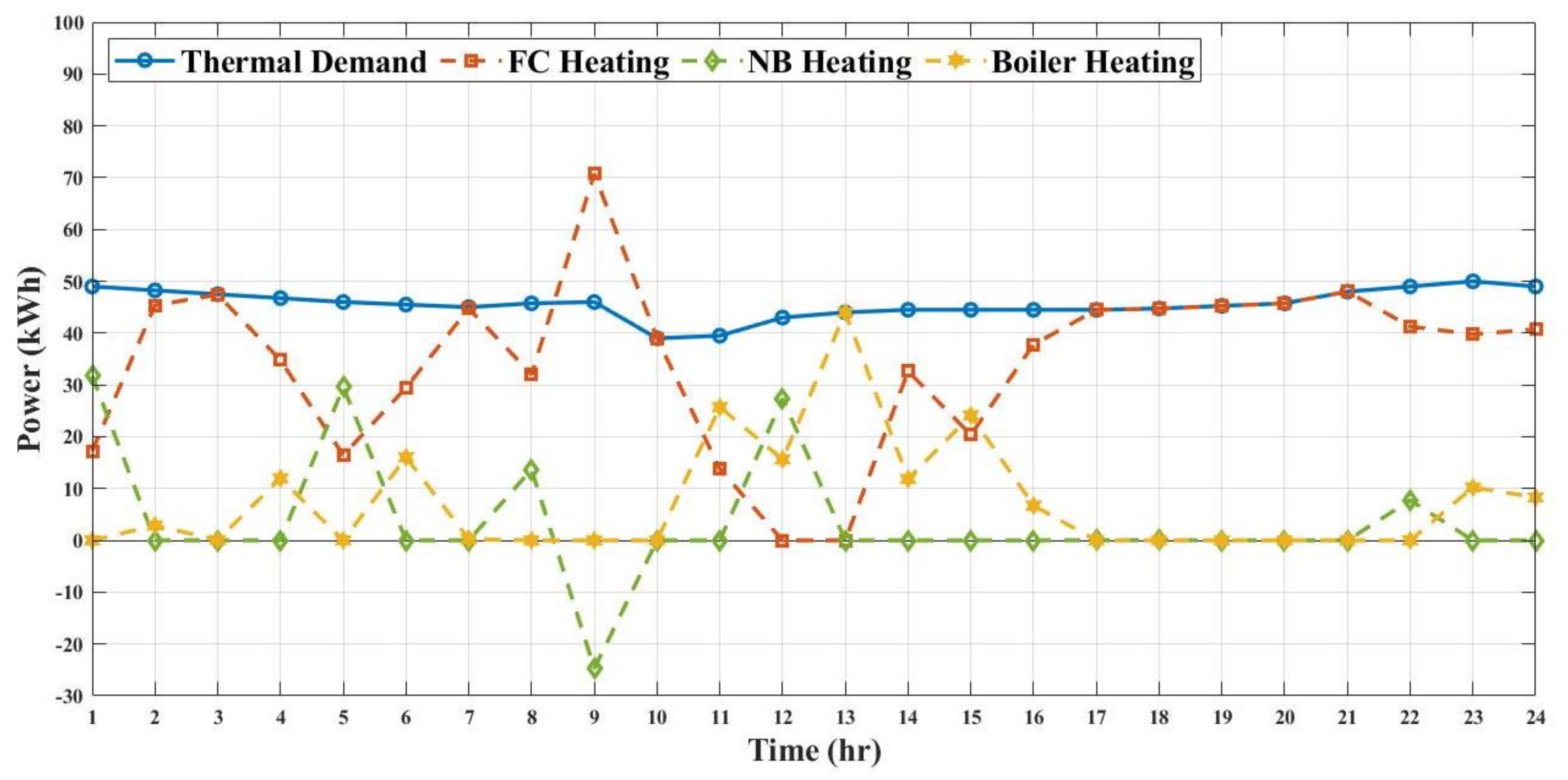
5.8. Case 7: Addition of Heat Storage Tank (HST)
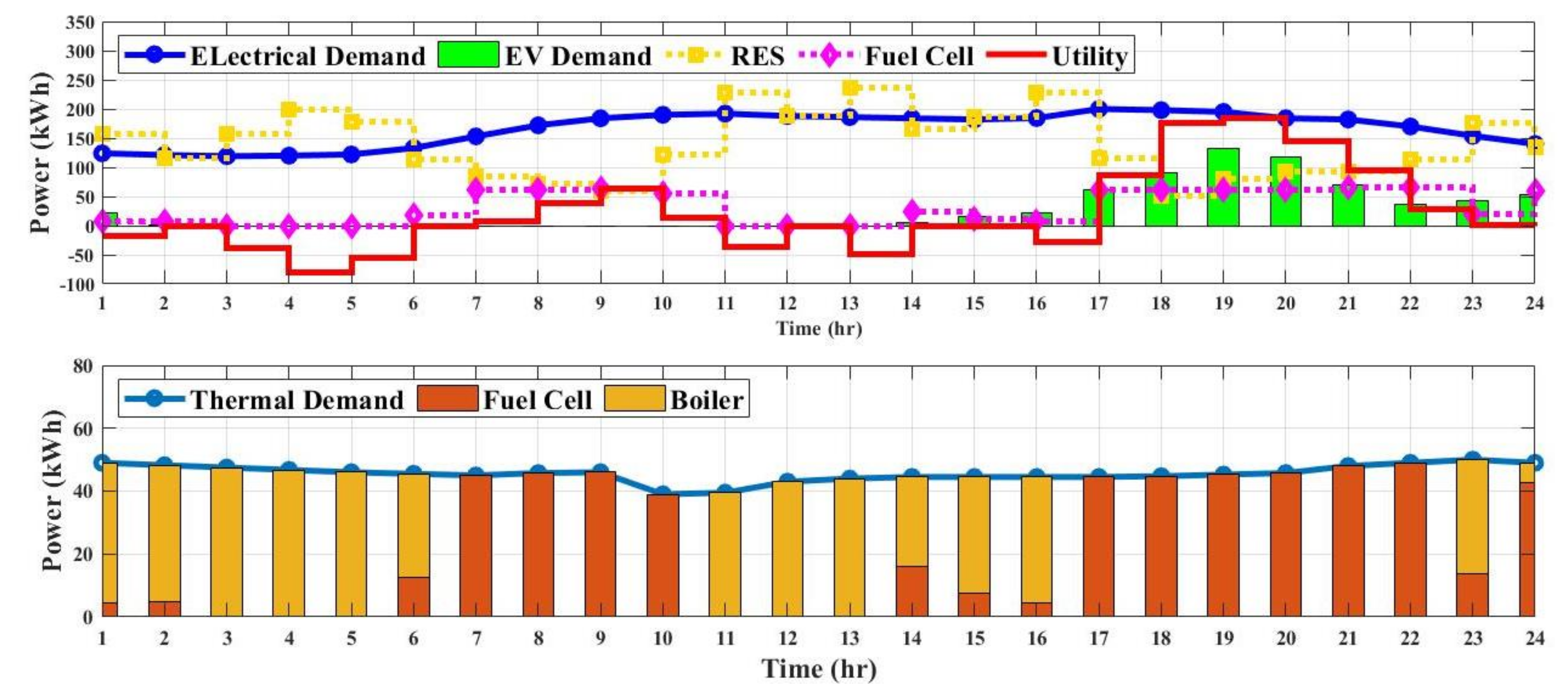
In this strategy, HST is installed in the SB. It works along with NSB energy buying and selling capability of the SB. The deficient power is also supplied by the AB. Figure 18 and Figure 19 depict the electrical and thermal powers of the SB respectively in this case. Similar to other strategies, the utility is complementing the FC electrical output in this case also. FC efficiency is higher in the middle hours of the day as compared to the starting and ending hours.
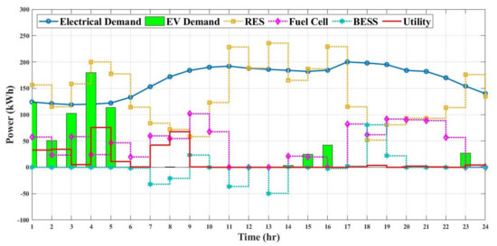
Figure 18.
Electrical powers for Case 7.
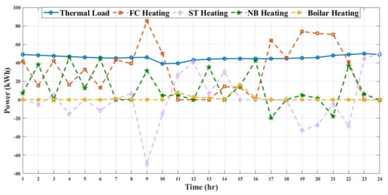
Figure 19.
Thermal powers for Case 7.
In the initial hours, between 1:00–10:00, the thermal energy usage and generation pattern are similar to the previous case. Thermal loading is more than FC thermal output and HST does not find any energy to store. The initial energy in the HST is considered zero; therefore, it does not provide any heating either. From 1:00 to 10:00 hours, the system buys heat from the NSB as much as available and, at 11:00, it buys according to its needs. Some of this heat is being provided to fulfill the needs of the SB and the remainder is being stored in the HST. Further heat storage in the HST starts at 12:00 p.m. when SB heat requirement decreases. The excessive thermal heating of the FC now stores in the HST. The storage of energy in the HST ends at 5:00 p.m. The SBEMS ensures that the HST is full from optimally storing the available energy from the FC and from the NSB before 6:00 p.m. ( when demand exceeds the FC output again) as shown in Figure 19. The net energy cost of SB in this case is 176.62$/day, which is 73.19% less than the base case and 2.30% less than the previous case.
Table 5 provides the cost of Utility, Boiler, Fuel Cell, and Neighborhood heat sharing for each case. It is clear from the table that Case 7 has the lowest cost as compared to the Base Case and all other cases. Table 6 illustrates the numerical values of the power demands and generations, and Table 7 provides 24-h operation cost of the smart building. The utility, FC, and boiler are mainly responsible for the total cost of operation on the smart building, whereas the operation and maintenance cost of battery and heat storage tank are negligible (i.e., $0.0062 per day).
Table 5.
Costs comparison table.
Table 6.
24 h power demands and generations.
Table 7.
24 h cost of the smart building.
6. Conclusions and Future Work
In the fight against climate change, with many global economies setting mid-century net zero carbon reduction targets, the pressure is on to develop strategies to bring down emissions in our cities, save energy, and speed up the transition to renewable energy. Therefore, using hybrid energy resources can play a significant role in not only reducing the reliance on fossil fuel depletable resources, but it can also bring a significant change in improving the environment both at global and regional levels. This research work has mainly focused on designing and modeling an SBEMS in the context of modern smart buildings to optimize their economic operation by utilizing RCGA which demonstrates the efficient usage of renewable energy resources in conjunction with grid connected energy resources which can potentially create a new ecosystem that can rely more on renewable energy, saving energy cost, minimising energy waste, and slashing carbon emissions.
In order to fulfil the electrical and thermal needs, the proposed SB model includes a hybrid energy system which incorporates electric power from a bidirectional utility, BSS, wind turbine, and a PV system as well as a thermal system including a natural gas fired fuel cell based CHP system, auxiliary boiler, heat exchange from neighbourhood buildings, and a heat storage tank. The model for these system devices were presented and the constraint of electrical and thermal power balance, minimum and maximum capacity constraints of the BSS, EV, storage tank and neighbourhood heat sharing were also modelled along with the maximum charging rate and discharging rate constraints of these devices. The FC’s start-up and shut-down costs and its ramp rate constraints were also considered. In this work, a bidirectional utility grid is considered where the building can sell out their surplus power to the grid. A typical EV charging scheduling was added, and their impact on the building economy was considered, keeping in mind the large loading implications of EVs. Different heating strategies were also incorporated for thermal load management. The system was optimized using a real coded genetic algorithm which gives optimal scheduling of hybrid energy resources to minimize the cost of 24-h energy consumption. According to simulation results, the proposed SBEMS optimally scheduled energy resources and EV charging at the same time, resulting in a cost-effective economic operation of the SB. To demonstrate the features of the proposed model, a comparison of the costs and savings of SB devices was summarized. The inclusion of RES, FC, and BSS resulted in 63.48%, 11.70%, and 4.30% reduction in energy costs, respectively. The scheduling of EV charging further reduces the cost by 9.31%; the inclusion of HST and NSB buying and selling resulted in better thermal energy routing and reduced the cost by 4.09% and 2.30%, respectively. This study shows that optimal usage of HES enhanced the economy of SB while reducing the utility dependency in the presence of EVs. It is evident from the simulation that the recommended SBEMS optimally schedules energy resources and loads to minimize the daily operating cost of the smart building. The effectiveness of the proposed formulation has been validated by means of various case studies, which have configured the efficient performance of this formulation. This work maybe unfold in the future to incorporate stochastic analysis of various components of SB. Furthermore, the benefits of SBEMS from the environmental aspect can further be investigated and analyzed. Similarly, considering bidirectional energy flow from electric vehicle (V2B and B2V) in the proposed model may yield interesting results. An optimal sizing of the CHP system and HST can also be performed for enhanced coordination of the installed devices and a better economy. A Matlab GUI could also be built that might select various devices, takes system parameters of the user choice, and generate the optimal cost by economically dispatching the installed devices.
Author Contributions
Conceptualization, M.H.K. and A.U.A.; methodology, M.H.K., N.U. and M.K.R.; software, M.H.K., M.K.R. and F.R.A.; validation, A.U.A., N.U., F.R.A. and M.K.R.; formal analysis, M.H.K.; investigation, M.H.K.; resources, N.U., F.R.A. and M.K.R.; data curation, M.H.K. and A.U.A.; writing—original draft preparation, M.H.K.; writing—review and editing, M.H.K., A.U.A. and M.K.R. All authors have read and agreed to the published version of the manuscript.
Funding
The authors would like to acknowledge the support from Taif University Researchers Supporting Project Number (TURSP-2020/331), Taif University, Taif, Saudi Arabia.
Conflicts of Interest
The authors declare no conflict of interest.
References
- Salam, R.A.; Amber, K.P.; Ratyal, N.I.; Alam, M.; Akram, N.; Gómez Muñoz, C.Q.; García Márquez, F.P. An Overview on Energy and Development of Energy Integration in Major South Asian Countries: The Building Sector. Energies 2020, 13, 5776. [Google Scholar] [CrossRef]
- Ahmad, T.; Zhang, D. A critical review of comparative global historical energy consumption and future demand: The story told so far. Energy Rep. 2020, 6, 1973–1991. [Google Scholar] [CrossRef]
- Yumashev, A.; Ślusarczyk, B.; Kondrashev, S.; Mikhaylov, A. Global indicators of sustainable development: Evaluation of the influence of the human development index on consumption and quality of energy. Energies 2020, 13, 2768. [Google Scholar] [CrossRef]
- Simões, N.; Manaia, M.; Simões, I. Energy performance of solar and Trombe walls in Mediterranean climates. Energy 2021, 234, 121197. [Google Scholar] [CrossRef]
- Fiaschi, D.; Bertolli, A. Design and exergy analysis of solar roofs: A viable solution with esthetic appeal to collect solar heat. Renew. Energy 2012, 46, 60–71. [Google Scholar] [CrossRef]
- Lohmann, V.; Santos, P. Trombe Wall Thermal Behavior and Energy Efficiency of a Light Steel Frame Compartment: Experimental and Numerical Assessments. Energies 2020, 13, 2744. [Google Scholar] [CrossRef]
- Hu, Z.; He, W.; Ji, J.; Zhang, S. A review on the application of Trombe wall system in buildings. Renew. Sustain. Energy Rev. 2017, 70, 976–987. [Google Scholar] [CrossRef]
- Zhang, H.; Tao, Y.; Shi, L. Solar Chimney Applications in Buildings. Encyclopedia 2021, 1, 409–422. [Google Scholar] [CrossRef]
- Kaygusuz, A. Closed loop elastic demand control by dynamic energy pricing in smart grids. Energy. 2019, 176, 596–603. [Google Scholar] [CrossRef]
- Davatgaran, V.; Saniei, M.; Mortazavi, S.S. Smart distribution system management considering electrical and thermal demand response of energy hubs. Energy 2019, 169, 38–49. [Google Scholar] [CrossRef]
- Martirano, L.; Rotondo, S.; Kermani, M.; Massarella, F.; Gravina, R. Power Sharing Model for Energy Communities of Buildings. IEEE Trans. Ind. Appl. 2021, 57, 170–178. [Google Scholar] [CrossRef]
- Zhou, B.; Li, W.; Chan, K.W.; Cao, Y.; Kuang, Y.; Liu, X.; Wang, X. Smart home energy management systems: Concept, configurations, and scheduling strategies. Renew. Sustain. Energy Rev. 2016, 61, 30–40. [Google Scholar] [CrossRef]
- Sanguinetti, A.; Karlin, B.; Ford, R.; Salmon, K.; Dombrovski, K. What’s energy management got to do with it? Exploring the role of energy management in the smart home adoption process. Energy Effic. 2018, 11, 1897–1911. [Google Scholar] [CrossRef] [Green Version]
- Ford, R.; Pritoni, M.; Sanguinetti, A.; Karlin, B. Categories and functionality of smart home technology for energy management. Build. Environ. 2017, 123, 543–554. [Google Scholar] [CrossRef] [Green Version]
- Moya, F.; Torres-Moreno, J.; Álvarez, J. Optimal Model for Energy Management Strategy in Smart Building with Energy Storage Systems and Electric Vehicles. Energies 2020, 13, 3605. [Google Scholar] [CrossRef]
- Ahmad, M.; Javaid, N.; Niaz, I.A.; Almogren, A.; Radwan, A. A Cost-Effective Optimization for Scheduling of Household Appliances and Energy Resources. IEEE Access 2021, 9, 160145–160162. [Google Scholar] [CrossRef]
- Erdinc, O.; Paterakis, N.G.; Mendes, T.D.P.; Bakirtzis, A.G.; Catalao, J.P.S. Smart Household Operation Considering Bi-Directional EV and ESS Utilization by Real-Time Pricing-Based DR. IEEE Trans. Smart Grid 2014, 6, 1281–1291. [Google Scholar] [CrossRef]
- Chen, L.; Xu, Q.; Yang, Y.; Song, J. Optimal energy management of smart building for peak shaving considering multi-energy flexibility measures. Energy Build. 2021, 241, 110932. [Google Scholar] [CrossRef]
- Thomas, D.; Deblecker, O.; Bagheri, A.; Ioakimidis, C.S. A scheduling optimization model for minimizing the energy demand of a building using electric vehicles and a micro-turbine. In Proceedings of the 2016 IEEE International Smart Cities Conference (ISC2), Trento, Italy, 12–15 September 2016. [Google Scholar] [CrossRef]
- Thomas, D.; Deblecker, O.; Genikomsakis, K.; Ioakimidis, C.S. Smart house operation under PV and load demand uncertainty considering EV and storage utilization. In Proceedings of the IECON 2017—43rd Annual Conference of the IEEE Industrial Electronics Society, Beijing, China, 29 October–1 November 2017. [Google Scholar] [CrossRef]
- Mistry, R.D.; Eluyemi, F.T.; Masaud, T.M. Impact of aggregated EVs charging station on the optimal scheduling of battery storage system in islanded microgrid. In Proceedings of the 2017 North American Power Symposium (NAPS), West, VA, USA, 17–19 September 2017. [Google Scholar] [CrossRef]
- Mouli, G.R.C.; Kefayati, M.; Baldick, R.; Bauer, P. Integrated PV Charging of EV Fleet Based on Energy Prices, V2G, and Offer of Reserves. IEEE Trans. Smart Grid 2017, 10, 1313–1325. [Google Scholar] [CrossRef]
- García-Villalobos, J.; Zamora, I.; San Martín, J.I.; Asensio, F.J.; Aperribay, V. Plug-in electric vehicles in electric distribution networks: A review of smart charging approaches. Renew. Sustain. Energy Rev. 2014, 38, 717–731. [Google Scholar] [CrossRef]
- Ashique, R.H.; Salam, Z.; Aziz, M.J.B.A.; Bhatti, A.R. Integrated photovoltaic-grid dc fast charging system for electric vehicle: A review of the architecture and control. Renew. Sustain. Energy Rev. 2017, 69, 1243–1257. [Google Scholar] [CrossRef]
- Dubey, A.; Santoso, S. Electric Vehicle Charging on Residential Distribution Systems: Impacts and Mitigations. IEEE Access 2015, 3, 1871–1893. [Google Scholar] [CrossRef]
- Liu, H.; Wang, B.; Wang, N.; Wu, Q.; Yang, Y.; Wei, H.; Li, C. Enabling strategies of electric vehicles for under frequency load shedding. Appl. Energy 2018, 228, 843–851. [Google Scholar] [CrossRef]
- Jin, C.; Sheng, X.; Ghosh, P. Energy efficient algorithms for Electric Vehicle charging with intermittent renewable energy sources. In Proceedings of the 2013 IEEE Power Energy Society General Meeting, Vancouver, BC, Canada, 21–25 July 2013; pp. 1–5. [Google Scholar] [CrossRef]
- Domínguez-Navarro, J.; Dufo-López, R.; Yusta-Loyo, J.; Artal-Sevil, J.; Bernal-Agustín, J. Design of an electric vehicle fast-charging station with integration of renewable energy and storage systems. Int. J. Electr. Power Energy Syst. 2019, 105, 46–58. [Google Scholar] [CrossRef]
- Choi, S.H.; Hussain, A.; Kim, H.M. Adaptive Robust Optimization-Based Optimal Operation of Microgrids Considering Uncertainties in Arrival and Departure Times of Electric Vehicles. Energies 2018, 11, 2646. [Google Scholar] [CrossRef] [Green Version]
- Angrisani, G.; Canelli, M.; Roselli, C.; Sasso, M. Integration between electric vehicle charging and micro-cogeneration system. Energy Convers. Manag. 2015, 98, 115–126. [Google Scholar] [CrossRef]
- Yokoyama, T.W.N.W.R. Energy-saving effect of a residential polymer electrolyte fuel cell cogeneration system combined with a plug-in hybrid electric vehicle. Energy Convers. Manag. 2014, 40–51. [Google Scholar] [CrossRef]
- Yokoyama, T.W.N.W.R. Feasibility study on combined use of residential SOFC cogeneration system and plug-in hybrid electric vehicle from energy-saving viewpoint. Energy Convers. Manag. 2012, 170–179. [Google Scholar] [CrossRef]
- Entchev, H.R.E. Exploring the potential synergy between micro-cogeneration and electric vehicle charging. Appl. Therm. Eng. 2014, 677–685. [Google Scholar]
- Khan, S.U.; Mehmood, K.K.; Haider, Z.M.; Bukhari, S.B.A.; Lee, S.J.; Rafique, M.K.; Kim, C.H. Energy Management Scheme for an EV Smart Charger V2G/G2V Application with an EV Power Allocation Technique and Voltage Regulation. Appl. Sci. 2018, 8, 648. [Google Scholar] [CrossRef] [Green Version]
- Benam, M.R.; Madani, S.S.; Alavi, S.M.; Ehsan, M. Optimal Configuration of the CHP System Using Stochastic Programming. IEEE Trans. Power Deliv. 2015, 30, 1048–1056. [Google Scholar] [CrossRef]
- El-Sharkh, M.Y.; Rahman, A.; Alam, M.S.; El-Keib, A.A. Thermal energy management of a CHP hybrid of wind and a grid-parallel PEM fuel cell power plant. In Proceedings of the 2009 IEEE/PES Power Systems Conference and Exposition, Seattle, WA, USA, 15–18 March 2009; pp. 1–6. [Google Scholar]
- Nehrir, M.H.; Wang, C. Hybrid Fuel Cell Based Energy System Case Studies. In Modeling and Control of Fuel Cells:Distributed Generation Applications; Wiley-IEEE Press: Hoboken, NJ, USA, 2009; pp. 219–264. [Google Scholar] [CrossRef]
- Adam, A.; Fraga, E.S.; Brett, D.J. Options for residential building services design using fuel cell based micro-CHP and the potential for heat integration. Appl. Energy 2015, 138, 685–694. [Google Scholar] [CrossRef]
- Xie, D.; Lu, Y.; Sun, J.; Gu, C.; Li, G. Optimal Operation of a Combined Heat and Power System Considering Real-time Energy Prices. IEEE Access 2016, 4, 3005–3015. [Google Scholar] [CrossRef]
- Feng, Z.B.; Jin, H.G. Part-load performance of CCHP with gas turbine and storage system. In Proceedings of the Chinese Society for Electrical Engineering, Turtle Bay, HI, USA, 19–21 April 2006; 26, pp. 25–30. [Google Scholar]
- Cao, Y.; Tang, S.; Li, C.; Zhang, P.; Tan, Y.; Zhang, Z.; Li, J. An Optimized EV Charging Model Considering TOU Price and SOC Curve. IEEE Trans. Smart Grid 2012, 3, 388–393. [Google Scholar] [CrossRef]
- Romano, R.; Siano, P.; Acone, M.; Loia, V. Combined Operation of Electrical Loads, Air Conditioning and Photovoltaic-Battery Systems in Smart Houses. Appl. Sci. 2017, 7, 525. [Google Scholar] [CrossRef] [Green Version]
- Mohsenian-Rad, H.; Ghamkhari, M. Optimal Charging of Electric Vehicles With Uncertain Departure Times: A Closed-Form Solution. IEEE Trans. Smart Grid 2015, 6, 940–942. [Google Scholar] [CrossRef]
- Saeed Uz Zaman, M.; Bukhari, S.B.A.; Hazazi, K.M.; Haider, Z.M.; Haider, R.; Kim, C.H. Frequency Response Analysis of a Single-Area Power System with a Modified LFC Model Considering Demand Response and Virtual Inertia. Energies 2018, 11, 787. [Google Scholar] [CrossRef] [Green Version]
- Haider, Z.M.; Mehmood, K.K.; Rafique, M.K.; Khan, S.U.; Soon-Jeong, L.; Chul-Hwan, K. Water-filling algorithm based approach for management of responsive residential loads. J. Mod. Power Syst. Clean Energy 2018, 6, 118–131. [Google Scholar] [CrossRef] [Green Version]
- Yao, L.; Damiran, Z.; Lim, W.H. Optimal Charging and Discharging Scheduling for Electric Vehicles in a Parking Station with Photovoltaic System and Energy Storage System. Energies 2017, 10, 550. [Google Scholar] [CrossRef]
- Gunes, M.B. Investigation of a fuel cell based total energy system for residential applications. Ph.D. Thesis, Virginia Tech, Blacksburg, VA, USA, 2001. [Google Scholar]
- The U.S. Electric Vehicle Industry—Statistics & Facts. Available online: https://www.statista.com/topics/4421/the-us-electric-vehicle-industry/#dossierKeyfigures (accessed on 27 June 2021).
- 2021 Nissan LEAF Specs & Prices|Nissan USA. Available online: https://www.nissanusa.com/vehicles/electric-cars/leaf/specs/compare-specs.html#modelName=S|40%20kWh (accessed on 27 June 2021).
- Chevrolet Bolt EV–2019. Available online: https://www.chevrolet.com/electric/bolt-ev (accessed on 27 June 2021).
- Kia Soul EV Specs|Compact Electric Car|Kia Motors Aruba. Available online: https://www.kia.com/aw/showroom/soul-ev/specification.html (accessed on 27 June 2021).
- Model 3|Tesla. Available online: https://www.tesla.com/model3 (accessed on 27 June 2021).
- National Household Travel Survey 2021. Available online: https://nhts.ornl.gov/ (accessed on 27 June 2021).
- Li, Y.; Xie, K.; Wang, L.; Xiang, Y. The impact of PHEVs charging and network topology optimization on bulk power system reliability. Electr. Power Syst. Res. 2018, 163, 85–97. [Google Scholar] [CrossRef]
- Wu, X.; Hu, X.; Yin, X.; Moura, S.J. Stochastic Optimal Energy Management of Smart Home With PEV Energy Storage. IEEE Trans. Smart Grid 2018, 9, 2065–2075. [Google Scholar] [CrossRef]
- Hu, Z.; Han, X.; Wen, Q. Integrated Resource Strategic Planning and Power Demand-Side Management; Power Systems; Springer: Berlin, Germany, 2013. [Google Scholar]
- Gianfreda, A.; Grossi, L. Zonal price analysis of the Italian wholesale electricity market. In Proceedings of the 2009 6th International Conference on the European Energy Market, Leuven, Belgium, 27–29 May 2009; pp. 1–6. [Google Scholar] [CrossRef]
- Gu, W.; Wu, Z.; Yuan, X. Microgrid economic optimal operation of the combined heat and power system with renewable energy. In Proceedings of the IEEE PES General Meeting, Atlanta, GA, USA, 25–29 July 2010; pp. 1–6. [Google Scholar] [CrossRef]
- Michalewicz, Z. Genetic Algorithms + Data Structures = Evolution Programs, 3rd ed.; Springer: London, UK, 1996. [Google Scholar]
- Damousis, I.G.; Bakirtzis, A.G.; Dokopoulos, P.S. Network-constrained economic dispatch using real-coded genetic algorithm. IEEE Trans. Power Syst. 2003, 18, 198–205. [Google Scholar] [CrossRef]
- Kuri-Morales, A.F.; Gutiérrez-García, J. Penalty Function Methods for Constrained Optimization with Genetic Algorithms: A Statistical Analysis. In MICAI 2002: Advances in Artificial Intelligence, Proceedings of the Second Mexican International Conference on Artificial Intelligence Mérida, Yucatán, Mexico, 22–26 April 2002; Coello Coello, C.A., de Albornoz, A., Sucar, L.E., Battistutti, O.C., Eds.; Springer: Berlin/Heidelberg, Germany, 2002; pp. 108–117. [Google Scholar] [CrossRef] [Green Version]
- Amjady, N.; Nasiri-Rad, H. Economic dispatch using an efficient real-coded genetic algorithm. IET Gener. Transm. Distrib. 2009, 3, 266–278. [Google Scholar] [CrossRef]
- Goldberg, D.E. Genetic Algorithms in Search, Optimization, and Machine Learning Artificial Intelligence; Addison-Wesley Publishing Company: New York, NY, USA, 1989. [Google Scholar]
- Ferragud, F.X.B. Control Predictivo Basado en Modelos Mediante Técnicas de Optimización Heurística. Aplicación a Procesos no Lineales y Multivariables. Ph.D. Thesis, Universitat Politècnica de València, Valencia, Spain, 1999. [Google Scholar]
- Herrera, F.; Lozano, M.; Verdegay, J.L. Tackling Real-Coded Genetic Algorithms: Operators and Tools for Behavioural Analysis. Artif. Intell. Rev. 1998, 12, 265–319. [Google Scholar] [CrossRef]
- Mühlenbein, H.; Schlierkamp-Voosen, D. Predictive Models for the Breeder Genetic Algorithm–I. Continuous Parameter Optimization. Evol. Comput. 1993, 1, 25–49. [Google Scholar] [CrossRef]
- De Jong, K.A. An Analysis of the Behavior of a Class of Genetic Adaptive Systems. Ph.D. Thesis, University of Michigan, Ann Arbor, MI, USA, 1975. [Google Scholar]
- Linkevics, O.; Sauhats, A. Formulation of the objective function for economic dispatch optimisation of steam cycle CHP plants. In Proceedings of the 2005 IEEE Russia Power Tech, St. Petersburg, Russia, 27–30 June 2005; pp. 1–6. [Google Scholar] [CrossRef]


Publisher’s Note: MDPI stays neutral with regard to jurisdictional claims in published maps and institutional affiliations. |
© 2022 by the authors. Licensee MDPI, Basel, Switzerland. This article is an open access article distributed under the terms and conditions of the Creative Commons Attribution (CC BY) license (https://creativecommons.org/licenses/by/4.0/).