Abstract
To achieve the goal of achieving carbon-neutral by 2060, the government of China has put forward higher requirements for energy conservation and consumption reduction in the energy industry. Therefore, it is necessary to reduce energy consumption in the process of transporting oil. In this paper, an optimization model that minimizes the total energy consumption of the entire pipeline system is proposed and the squirrel search algorithm (SSA) is used to solve the optimization model. Meanwhile, to improve the performance of the SSA, two strategies are proposed. One is the adaptive inertia weight strategy, and the other is the multi-group co-evolution strategy. The adaptive inertia weight can adjust the step size of the flying squirrels according to the difference of the objective function value and multi-group co-evolution is introduced to improve population diversity. The improved SSA is named multigroup coevolution-adaptive inertia weight SSA (MASSA). A total of 20 benchmark functions are used to test the performance of MASSA, including unimodal functions and multimodal functions. Compared with the other four algorithms, MASSA has better performance and convergence capabilities. In the case study experiment, an optimization model of the oil pipeline is built, which takes the minimum energy consumption of the whole pipeline as the objective function. Compared with the actual operating conditions, the electricity consumption optimized by MASSA decreases by 399,018.94 kgce, and the thermal energy dissipation decreases by 113,759.25 kgce. The total energy consumption is reduced by 512,778.19 kgce, which is 9.62%. These results indicate that the two improvement strategies are significant, and optimizing the operating parameters can reduce energy consumption.
1. Introduction
China strives to achieve the peak of carbon dioxide emissions by 2030 and carbon neutrality by 2060. How to achieve high-quality carbon peak and carbon-neutral goals has become an inevitable requirement for the development and transformation of China’s energy structure in the future. To achieve this goal, both energy production and transportation links must move toward a green and low-carbon path. Additionally, crude oil of the Qingtie Fourth-line has the characteristics of high viscosity and is easy to condense, and needs to be heated before being transported. Therefore, it needs to consume a lot of energy. Moreover, if the pipeline operating parameters do not meet the conditions, it will not only increase energy consumption and operating expenses but also cause the risk of pipeline condensation [1,2,3,4]. Therefore, it is meaningful to save energy and reduce consumption by adjusting the operating parameters of the pump.
In recent years, plenty of research has been carried out on reducing the energy consumption of oil pipeline transportation. These studies first establish the optimization model of the oil and gas pipeline system and then solve these models to find the fit operating parameters. In 2016, Jia et al. used the vacuum furnace dilution effect and uniform temperature disturbance to increase the water flow velocity in the heat exchange tube, which effectively extended the fouling time and maintenance cycled of the boiler pipe [5]. In 2017, Zhang et al proposed a model that took the minimum total cost of the energy assumption as the objective function, and due to more comprehensive considerations, the model was more practicable but also more complex [6]. In the same year, He et al. proposed to replace traditional heaters with high-temperature heat pumps, and replace traditional heating furnaces with high-temperature hot water to heat crude oil, reducing energy consumption [7]. Later, Liu et al adopted frequency control technology. In this way, a part of the energy wasted due to the adjustment of the outlet pressure regulating valve could be reduced, and due to the effective matching of motor output power and pipe flow, the energy consumption could be saved by 20~50%. Especially under the condition of low-flow pipeline operating, the application of this technology could produce more obvious economic benefits [8], and to better reflect the true and effective utilization of energy consumption, Cheng et al. took the unavoidable exergy loss rate as the evaluation index. The experiment results showed that the influence degree on the exergy loss rate in turn was: outbound temperature, flow, and outbound pressure [9]. In 2019, Liu et al analyzed the exergy loss and exergy efficiency of every component of the crude oil pipeline transportation system based on energy quality. The equipment arrangement and operating parameters of each station in the pipeline transportation system were optimized, and the results showed that the total oil transportation cost and the total exergy loss of the pipeline transportation system after optimization had seen an obvious improvement [10]. In 2020, Liu et al proposed an optimization model with compressor speed as a variable. The optimization results showed that not only the energy consumption was greatly reduced but also the pressure curve and temperature curve were more stable [11]. In 2022, Liu optimized and analyzed the transformed QT oil pipeline under the premise of ensuring safe production. The total energy consumption of the scheme optimized is reduced by 8.32%, the oil consumption is reduced by 7.99%, and the electricity consumption is reduced by 9.01% [12]. It can be seen from the above literature that adjusting the operating parameters of the pump or other equipment can effectively save energy. Moreover, discovered through data research, the ambient temperature near the Qingtie Fourth-line pipe is relatively low and the crude oil is highly viscous. In addition, there are multiple pumps in pumping stations, all of which are inverter pumps. Based on these conditions, an optimization model of the oil pipeline is proposed, which takes the minimum energy consumption of the whole pipeline as the objective function, and the variables are the speed of the invert pump, the pump unit combination mode, and the outlet temperature of the station. However, these parameters of the station are not isolated, it is difficult to empirically determine the operating parameters. Therefore, many heuristic algorithm solutions have been introduced.
The heuristic algorithm refers to a method of discovery based on empirical rules, such as genetic algorithm, particle swarm algorithm, and squirrel search algorithm [13,14,15]. Among them, SSA originated from the dynamic foraging and gliding behavior of flying squirrels [16], and a random search will be carried out that can improve the ability of the SSA greatly. In SSA, the hyper-parameter dg can effectively balance the exploitation capability and the exploration ability of SSA. Most heuristic algorithm solutions are easily falling into the local optimal. While compared with other heuristic algorithms, SSA can overcome this shortcoming to a certain extent because of its unique strategy. Therefore, it has been used in many fields and has been proven to be more effective for solving unimodal, multimodal, and multidimensional optimization problems [17,18,19,20,21]. However, SSA also has disadvantages. Therefore, some improvement measures have been implemented, which are shown in Table 1. Most of the literature mainly adjusts the value of predator presence probability or introduces another algorithm in SSA to improve its performance. In 2020, Zhang et al introduced a new parameter to adjust the step size of all squirrels [22]. While the calculated process of the new parameter was quite complicated, this parameter could not adjust the step size according to the position of every flying squirrel. Based on the above literature, an improved version of SSA called MASSA is proposed. In this paper, a new formula about dg is proposed, named adaptive inertia weight. This formula adjusts the value of the dg by measuring the difference in the fitness function value of each flying squirrel. Besides, the multi-group co-evolution is introduced to ensure population diversity, which can prevent SSA from falling into the local optimal in advance.

Table 1.
The results of some research in recent years.
This paper builds an optimization model that minimizes the total energy consumption of the entire pipeline system, as shown in Section 2, and, the optimization variables are the speed of the invert pump, the pump unit combination mode, and the outlet temperature of the station. The details of MASSA are shown in Section 3, and in Section 4, the performance of MASSA is verified by 20 test benchmark functions. In addition, this paper uses MASSA to solve the optimization model and analyzes the relationship between the optimization variables and the energy consumption.
2. Optimization Model
In this part, the objective function, the optimization variables, and the constraint conditions are introduced. This study is mainly based on the following assumptions:
- The conveying medium flows stably in the pipe;
- Single-phase (liquid phase) homogeneous flow of conveying medium in the pipe;
- The temperature of the conveying medium in the pipe is constant along the radial direction, and only the change of the axial temperature is considered.
2.1. Inverter Pump Processing
In this paper, to simulate the actual operating performance of the inverter pump, the flow-head equation and flow-power equation of the oil pump with the frequency converter are established based on multivariate linear formula, and the relationship between pressure head and power and flow rate and rotational speed. Meanwhile, the least square method is used to return the performance of the oil pump to a polynomial description. The flow-head and flow-power of the oil pump with the frequency converter are defined as the relationship between Equations (1) and (2). After many tests, it is found that this type of equation has the smallest error.
The flow-head relationship fitting equation of the inverter pump is as follows:
where H-Head provided by pump station [m]; A1, A2, A3, A4, A5, A6-The coefficient of the fitting equation of the relationship between flow and head, and the corresponding data of each station; Q-Volume flow of fluid [m3/s]; rs-Speed of invert pump in the ith pumping station [L/min].
The flow-power relationship fitting equation of the oil pump is as follows:
where P-Power provided by pump station [kW]; a1, a2, a3, a4, a5, a6-The coefficient of the fitting equation of the relationship between flow and head, and the corresponding data of each station; Q-Volume flow of fluid [m3/s]; rs-Speed of invert pump in the ith pumping station [L/min].
In addition, in this paper, station 1, 4, 6, and 7 have the same type of oil pumps, and the oil pumps of stations 3 and 5 are of the same model. Furthermore, there are no pumps in the station 2, 8, and 9. The fitting method used in this paper has high precision, with the error of the pressure head fitting within 5% and the power fitting error within 5%, and the fitting results are shown in Table 2.
Table 2.
The fitting results.
In Table 3, there are some related parameters of oil pumps at each station, and the simulation results of the model must be within the range of these parameters, otherwise it will not have practical value.
Table 3.
Related parameters of oil pumps at each station.
2.2. Objective Function
In the crude oil pipeline, the electricity consumption of the pump station and the thermal energy dissipation of the heating furnace are usually regarded as the main energy consumption. This model is based on the actual operating condition of the Qingtie Fourth-line. The objective function is the lowest energy consumption of the pipeline system in this paper [9,11].
where F—Pipeline energy consumption [kgce]; Se—Electricity consumption, [kgce]; Sh—Fuel consumption [kgce].
Electricity consumption Se can be expressed as:
where Np—the number of pump stations; G—the mass flow of crude oil in the pipe [kg/s]; —electricity conversion standard coal coefficient [0.1229 kgce/(kW h)]; Hi—head provided by pump station i [m]; g—acceleration constant of gravity [9.8 m/s2]; tpi—running time of pump station number i [h]; —mechanical efficiency and motor efficiency of the pump station numbered i.
Thermal energy dissipation Sh is shown as follow:
where Nh—the number of heating stations; G—the mass flow of crude oil in the pipe [kg/s]; —oil conversion standard coal coefficient [1428.6 kgce/t]; —specific heat capacity of the heated medium [kJ/(kg °C)]; —inlet and outlet temperature of heating station number i; —running time of heating station number i; —heating efficiency of the heating station; —low heating value of fuel [kJ/kg].
2.3. Optimization Variables
Through literature research and data collection, this paper finally chooses the speed of the invert pump, the pump unit combination mode of the pump station, and the outlet temperature of the station as the optimization variables.
where —pump unit combination mode of the ith pump station; rsi—speed of variable frequency pump of the pump unit in the ith pumping station; —the outbound temperature of heating station number i.
2.4. Calculation Process and Constrain
In this paper, to ensure the reliability of optimization results, eight constraint conditions are proposed. The main constraint conditions contain five aspects. The optimization model calculation process and the constraint conditions are shown in Figure 1. Besides, all the pump combinations are in series in the pump station, and the mode of three in use and one for standby is adopted.
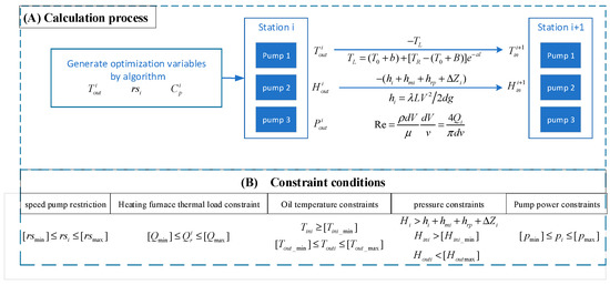
Figure 1.
Calculation process and constrain conditions.
3. Optimization Algorithm
3.1. Squirrel Search Algorithm
SSA is proposed based on the dynamic foraging and gliding behavior of flying squirrels [16]. It has a unique iteration mechanism, and the steps of SSA are as follow:
Step 1: Generate the initial population
The initial location of ith flying squirrel (FS) which distribute randomly in a forest is generated.
Step 2: Calculate objective function value
The objective function values of each flying squirrel are calculated, and there are three kinds of trees in the forest, hickory tree, acorn tree, and normal tree.
Step 3: Sort and Classify
The objective function values are sorted in ascending order. The flying squirrel with the global optimal value is assigned to the hickory nut tree. The next three best flying squirrels are on the acorn nuts trees. The rest of the flying squirrels are supposed to be on normal trees. This natural behavior is modeled by employing the location updating mechanism with predator presence probability.
Step 4: Regenerate new locations
- 1.
- Flying squirrels on acorn nut trees () will move toward hickory nut tree. In this case, the new location of squirrels can be obtained as follows:
where dg-a random gliding distance in the range [0.5, 1.1]. Gc is a constant that helps to balance exploration and exploitation capabilities in the model and in this paper the initial values of Gc is considered as 1.9. R1 is a random number in the range [0, 1]. is the location of flying squirrel that reached hickory nut tree, t -the current iteration.
- 2.
- Some flying squirrels on normal nut trees () may move toward acorn nut tree. In this case, the new location of squirrels can be obtained as follows:
where dg-a random gliding distance in the range [0.5, 1.1]. Gc is a constant that helps to balance exploration and exploitation capabilities in the model and in this paper the initial values of Gc is considered as 1.9. R1 is a random number in the range [0, 1]. is the location of flying squirrel that reached acorn nut trees, t-the current iteration.
- 3.
- The rest of the flying squirrels on normal nut trees will move toward hickory nut tree. In this case, the new location of squirrels can be obtained as follows:
where dg-a random gliding distance in the range [0.5, 1.1]. Gc is a constant that helps to balance exploration and exploitation capabilities in the model and in this paper the initial values of Gc is considered as 1.9. R1 is a random number in the range [0, 1]. is the location of flying squirrel that reached hickory nut tree, t- the current iteration.
Step 5: Seasonal monitoring condition
- 1.
- First calculate the seasonal constant () using Equation (10):
where t-the current iteration; is the location of flying squirrel that reached acorn nut trees; is the location of flying squirrel that reached hickory nut tree.
- 2.
- Calculate the minimum value of seasonal constant computed (Smin):
where t-the current iteration; tm-the maximum number of iterations.
When < Smin, the relocation of the remaining flying squirrel is modeled through Lévy distribution.
3.2. Multigroup Coevolution-Adaptive Inertia Weight SSA
In this paper, to improve the convergence efficiency of SSA and the searchability of the flying squirrel population, two strategies are utilized to improve SSA and named this improved SSA as MASSA. The details of MASSA are shown in Figure 2.
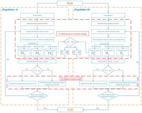
Figure 2.
MASSA algorithm frame.
3.2.1. Strategy 1: Multi-Group Co-Evolution
Co-evolution originated from the study of biology. In 1964, Ehrlich first put forward the concept of co-evolution when studying the relationship between butterflies and plants [27]. After that, it had been utilized in machine learning due to its characteristics [28,29,30,31,32].
There are two populations in MASSA, including population A and population B. As the iteration of MASSA continues, the global optimal flying squirrels in two populations will be compared, and the poor global optimal flying squirrel will be replaced by the better one. Additionally, at the beginning of the iteration process, this strategy can improve the population diversity, which can improve the searchability of SSA and avoid falling into local optima. Through many time tests, this paper finally chooses the dual populations’ system that performed relatively high in most cases.
3.2.2. Strategy 2: Adaptive Inertia Weight
In SSA, dg is an important constant, which is utilized to balance the exploitation capability and the exploration ability of SSA. Therefore, choosing a suitable dg can improve the performance of SSA. In 2021, Dalila et al. studied the influence of the dg parameter on algorithm performance. When dg is 0.85, the exploitation capability of SSA can be improved greatly, and when dg is 2.105, the SSA has excellent exploration ability [33]. The exploitation capability refers to the local optimization capability of the algorithm. While the exploration ability refers to the global optimization ability of the algorithm. In this paper, to balance the exploitation capability and the exploration ability of SSA, an adaptive inertia weight strategy is proposed. Through this strategy, the step size of flying squirrels close to the global optimal squirrel becomes smaller, so that these flying squirrels can carefully search the area around the global optimal. While the step size of these flying squirrels who are far away from the global optimal squirrel becomes longer, which can prevent the algorithm from over-converging in advance. The formula used in this strategy can be expressed as follow:
where dgi-a random gliding distance in the range [0.85, 2.105]; fi-the objective function value, , .
4. Experimental Set Up
4.1. Experimental Scheme Setting
In this part, this paper sets two experiments to verify the effectiveness of MASSA, and four heuristic algorithms are used for comparison. Experiment 1: A total of 20 well-known classic benchmark functions are taken to confirm the performance of MASSA. Experiment 2: Based on the Qingtie Fourth-line optimization model, which is established in Section 2, and MASSA is used to find the suitable pump operating parameters.
4.2. Experimental Parameters Setting
The parameters of the algorithms are shown in Table 4, and, to ensure the reliability of the results, the above two experiments are repeated 51 times, and the average results of 51 times are used for comparison. Besides, all the algorithms are implemented in PYCHARM 2019. All computations were run on a CPU: Intel(R) Core (TM)i5-6300HQ, 2.3 GHz, 8 G RAM, and Windows 10 (64-bit) operating system.
Table 4.
Parameters setting of algorithms.
5. Experimental Results and Analysis
5.1. Experiments on Function Study
In this paper, 20 benchmark functions are used to verify the effectiveness and applicability of the MASSA, which includes unimodal functions and multimodal functions [16,34]. The unimodal benchmark function contains only one optimal solution and is easy to solve. Therefore, they are often used to test the exploitation ability of algorithms. However, the multimodal functions have multiple local optimal solutions. Compared with unimodal benchmark functions, their global optimal is more difficult to obtain. It can be used to test the exploration ability of algorithms. Besides, as the number of N increases, it becomes more and more difficult to find the global optimal. The recorded results of statistical analysis are shown in Table 5 and Table 6, including the mean fitness values and standard deviation (SD). In addition, a convergence rate analysis on the benchmark functions is also carried out, which can reflect the performance of MASSA more clearly, and the convergence rate pictures are shown in Figure 3, Figure 4, Figure 5 and Figure 6, which can show the convergence performance of all algorithms.
Table 5.
Result of unimodal benchmark functions.
Table 6.
Result of multimodal benchmark functions.
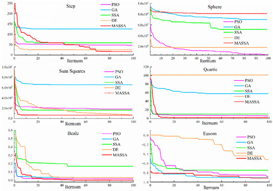
Figure 3.
Convergence results 1 of unimodal benchmark functions.
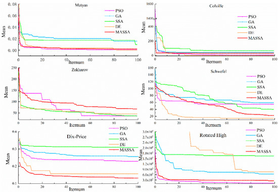
Figure 4.
Convergence results 2 of unimodal benchmark functions.
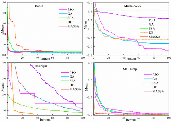
Figure 5.
Convergence results 1 of multimodal benchmark functions.
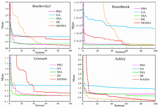
Figure 6.
Convergence results 2 of multimodal benchmark functions.
It can be seen from Table 5 that compared with the other four algorithms, the number of the smallest mean value in MASSA is more, especially when N is 30; as the test function becomes more complicated, the MASSA still has excellent performance and searchability. However, if the search range increase too much, the searchability of MASSA will drop sharply. The reason for this situation is that there are only 50 individuals in a population, so the single searchability of a single population has declined to a certain extent. In general, compared with SSA, the searchability of MASSA has been improved due to the adaptive inertia weight strategy and the multi-group co-evolution. Through these two strategies, the exploitation capability and exploration ability of MASSA have been well balanced. Meanwhile, the simulation results show the number of smallest SD in MASSA is as many as the PSO. This result shows that MASSA has great robustness. From Figure 3 and Figure 4, in most cases, all algorithms will converge within 100 generations. The convergence curve shows that, compared with other optimization methods, MASSA has superior convergence behavior with sufficient accuracy in comparison to other optimization methods. This is due to the multi-group strategy presence and the adaptive inertia weight in the search behavior of flying squirrels. The adaptive inertia weight can improve searchability by adjusting the step size of flying squirrels. Besides, the population diversity in MASSA can be guaranteed at the beginning. The above analysis results indicate that MASSA has an excellent performance in unimodal functions.
Table 6 shows the recorded results of statistical analysis of all algorithms in the multimodal benchmark functions. Figure 5 and Figure 6 show the convergence ability of the optimization algorithm in multimodal functions. From Table 6, it is evident from the results that MASSA is superior on Six Hump and Rastrigin. Besides, the MASSA also has the smallest mean values on Griewank and Ackley. These results show that the performance of MASSA on the multimodal function is still great. In addition, the performance of DE is also excellent on MichalEwicz, Boachevsky2, Rosenbrock, and Booth. In contrast, PSO is more stable than other optimization algorithms. It can be seen from Figure 5 and Figure 6 that the convergence ability of MASSA is also excellent. The reason is that the adaptive inertia weight can improve the searchability of the flying squirrels and prevent the algorithm from over-converging to a certain extent in advance. Additionally, the multi-group can also improve its searchability by improving its population diversity. These results show that the MASSA also can solve the multimodal functions.
The recorded results of statistical analysis show that all algorithms cannot find the global optimal. The reason is that the parameters, T, and population_size, are relatively small. The search range in the case study is relatively small and all algorithms will converge within 100 generations. If the parameter value is too large, it is equivalent to an exhaustive method, and there is not much actual use-value. In summary, the above analysis results show that the MASSA has excellent performance on unimodal function and multimodal functions. Besides, the convergence ability of MASSA is also great, which shows that the two improved strategies are effective. At the beginning of the algorithm iteration, the multi-group co-evolution strategy can ensure the population diversity, and this can prevent the MASSA from falling into the local optimal in advance. Meanwhile, through adaptive inertia weight, the step size of flying squirrels can be adjusted according to the difference of the fitness function value, which can balance the exploitation capability and the exploration ability effectively. These results show that is it feasible to solve the optimization model through MASSA.
5.2. Experiments on Case Study
To ensure the reliability of the result and convenience for comparison, a set of the actual operating data of the Qingtie Forth-line is collected in July 2018, as shown in Table 7 and Table A1 in Appendix A. Then, the optimized results by four algorithms are shown in Table 8 and Table A2, Table A3 and Table A4, and the Figure 7, Figure 8 and Figure 9 show the energy consumption, pressure changes and temperature changes in each station, respectively.
Table 7.
July actual operation scheme.
Table 8.
MASSA simulation operation scheme.
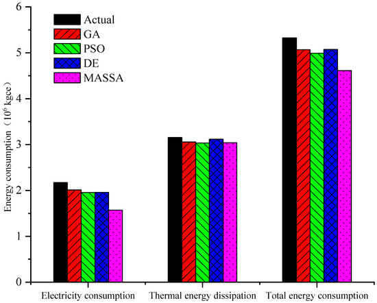
Figure 7.
Energy consumption comparison between the actual scheme and the four algorithms’ simulation operation schemes.
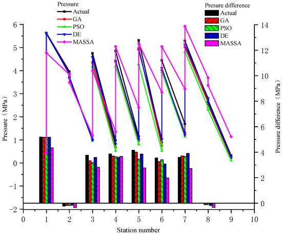
Figure 8.
Pressure comparison between the actual scheme and the four algorithms’ simulation operation schemes.
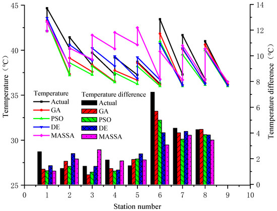
Figure 9.
Temperature comparison between the actual scheme and the four algorithms’ simulation operation schemes.
Form the Table 7 and Table A2, Table A3 and Table A4, compared with the actual operating situation, the total energy consumption of GA is reduced by 259,222.66 kgce, the total energy consumption of PSO is reduced by 334,900.94 kgce, the total energy consumption of DE is reduced by 252,988.57 kgce, and the total energy consumption of MASSA is reduced by 512,778.19 kgce, which is a reduction of 9.62%. From Figure 7, it can be seen that the reduction of electricity consumption is more obvious in these two types of energy consumption. Compared with the actual operating situation, the electricity consumption of GA, PSO, DE, and MASSA decrease by 161,228.22 kgce, 215,541.03 kgce, 214,985.33 kgce, and 399,018.94 kgce, respectively. In addition, the thermal energy dissipation of GA, PSO, DE, and MASSA decrease 97,994.44 kgce, 119,359.91 kgce, 38,003.24 kgce, and 113,759.25 kgce, respectively. Through analysis, it is found that although the number of pumps opened is the same, the speed of the pump changes, resulting in the total pressure drop in four algorithms being lower than the actual scheme. Besides, the total temperature drop in the four algorithms is lower than the actual scheme.
In Formula (4), the main variables related to electricity consumption are inlet pressure and out pressure. Therefore, this paper mainly analyzes the electricity consumption by comparing the inlet and outlet pressures of various oil transportation stations. It can be seen from Figure 8 that the pressure change trends of the optimized scheme and the actual scheme are extremely similar. In most stations, the inlet pressure optimized by algorithms is higher than the actual scheme. However, it is difficult to find out which scheme has less pressure energy consumption only based on the curve in the figure, because the outlet pressure of various schemes is not consistent. Therefore, this article uses the relevant data of each pumping station to calculate the total pressure drop of the pipe section. The total pressure drop of the actual scheme is 23.90 MPa. In GA, the total pressure drop is 22.89 MPa; in PSO, the total pressure drop is 22.27 MPa; in DE, the total pressure drop is 22.86 MPa; In MASSA, the total pressure drop is 19.65 MPa. In contrast, the total pressure drop optimized by MASSA is reduced by 4.25 MPa, which is 21.6%. In the pipe section, the main way to adjust the pressure in and out of the station is to change the speed of the pump or the number of pumps open. From Table 8 and Table A2, Table A3 and Table A4, the number of pumps of the actual scheme and four algorithms are the same. However, the speed of the pump decreases in station 3 and station 5~7. These results show that reducing the energy consumption is feasible through adjusting the operating parameters of the pumps and the results of optimization variables are of practical use value.
Formula (5) reveals that the thermal energy dissipation is related to the outlet temperature, the inlet temperature, and the flow. This paper mainly analyzes the total temperature drop to determine the optimization result. Form Figure 9, the total temperature drop of GA, PSO, DE, and MASSA is 20.89 °C, 18.83 °C, 20.75 °C, and 19.81 °C, respectively, and the total temperature drop of the actual scheme is 24.34 °C. Compared with the actual scheme, the total temperature drop optimized by MASSA is 4.53 °C, a drop of 18.6%. Therefore, choosing a suitable pipe temperature can not only save energy but also ensure the pipeline’s transport capacity.
It can be seen from the above analysis results that the optimization model is feasible. According to the simulation results, it is effective to reduce the energy consumption by optimizing the speed of the pump, the combination of the pump, and the outlet temperature of the pump. Through calculation, it can be known that under the same ratio, the reduction in electricity consumption is more obvious. This is because by adjusting the speed of the pump, the overall operating efficiency of the pump can be improved. Besides, the temperature in the area where the Qingtie Fourth Line is located is low, and the crude oil is high viscosity crude oil and is easy to condense. Therefore, the station should choose outlet temperature and reduce the heat exchange between the pipeline and the surrounding environment.
6. Conclusions
To reduce the operating energy consumption of Qingtie Fourth-line, this paper builds an optimization model of minimizing the total energy consumption of the whole pipeline system, and an improved heuristic algorithm named MASSA is proposed, which combined multi-group co-evolution strategy and adaptive inertia weight.
The statistical results of 20 benchmark functions show that the MASSA has excellent searchability and convergence performance in unimodal function and multimodal function. At the beginning of the iterative process, the multi-group co-evolution strategy can improve the population diversity, thereby ensuring searchability. However, due to too few individuals in each population, it affects the single searchability of the population to a certain extent. Besides, the adaptive inertia weight builds the relationship between the step size and the difference in the fitness function values. Therefore, adaptive inertia weight can effectively balance the exploitation capability and exploration ability of MASSA. These strategies can prevent the MASSA from over-converging to a certain extent in advance.
Besides, the optimization model is verified by the data of the Qingtie Fourth-line. Compared with the actual scheme, the total energy consumption optimized by MASSA is reduced by 512,778.19 kgce, which is a reduction of 9.62%, and the electricity consumption and thermal energy dissipation have been reduced by 399,018.94 kgce and 113,759.25 kgce, respectively. In MASSA, the total temperature drop is 19.81 °C and the total pressure drop is 19.65 MPa, and under the same ratio, the decrease in electricity consumption is more obvious. Therefore, in the actual operation of the Qingtie Fourth-line, the station should choose the fit operating parameters, including the speed of the pump, the combination of the pump, and the outlet temperature of the station. Besides, the station should set up enough insulation layers on the pipeline to reduce the heat exchange between the pipeline and the surrounding environment.
In this paper, an energy consumption optimization model of the oil transportation process is proposed with the pump as the main optimization variable. However, the station has a lot of production equipment. If these pieces of equipment can be considered in the model, the simulation results will be closer to the actual operation of the station and more reliable. In addition, the optimization algorithm should mainly consider its stability and solution accuracy when choosing it.
Author Contributions
Conceptualization, S.P.; methodology, S.P. and Z.Z.; software, Z.Z.; formal analysis, Y.J.; investigation, L.S.; writing—original draft preparation, Z.Z.; writing—review and editing, S.P.; funding acquisition, S.P. All authors have read and agreed to the published version of the manuscript.
Funding
This research was funded by CNPC science and technology major project, grant number: 2013B-3410.
Data Availability Statement
Not applicable.
Conflicts of Interest
The authors declare no conflict of interest.
Nomenclature
| Head provided by pump station ith | m | Reynolds number | |||
| Acceleration constant of gravity | 9.8 m/s2 | Fluid density | kg/m3 | ||
| Outlet temperature of heating station number ith | °C | d | Inside diameter of the pipe | m | |
| Inlet temperature of heating station number ith | °C | V | Flow rate of fluid in the pipeline | m/s | |
| Low heating value of fuel | KJ/kg | Dynamic viscosity | Pas | ||
| Speed of variable frequency pump of the pump unit in the ith pumping station | L/min | Qi | Volume flow of fluid in the pipeline | m3/s | |
| Oil temperature L meters from the start of the pipeline | °C | Friction loss along the line | m | ||
| The ground temperature of buried pipeline environment | °C | L | Length of pipe | m | |
| Oil temperature at the beginning of the pipeline | °C | d | Inside diameter of the pipe | m | |
| Thermal load of the ith heating station | KJ/kg | Friction coefficient | |||
| Rated heat load of the heating furnace (maximum heat load) | KJ/kg | Friction between pump stations | m | ||
| The minimum allowable speed of the pump | L/min | Local friction between pumping stations | m | ||
| The maximum speed allowed by the pump | L/min | Friction between heating stations | m | ||
| The outbound head of the ith pump station | m | Power of oil pump | kW | ||
| Maximum working head of pipeline | m | Inlet head of the ith pumping station | m | ||
| Minimum outbound temperature of the ith hot station | °C | Allowable minimum inlet head of the ith pumping station | m | ||
| Maximum outbound temperature of the ith hot station | °C | The outbound head of the ith pump station | m | ||
| Minimum heat load of the heating furnace | KJ/kg | Maximum working head of pipeline | m |
Appendix A
Table A1.
Heat transfer coefficient K and ground temperature between stations.
Table A1.
Heat transfer coefficient K and ground temperature between stations.
| Pipe Section between Stations | K (w/m2·K) | Ground Temperature (°C) |
|---|---|---|
| Station 1 to station 2 | 0.869 | 15.9 |
| Station 2 to station 3 | 0.970 | 16.5 |
| Station 3 to station 4 | 1.770 | 17.1 |
| Station 4 to station 5 | 1.815 | 17.1 |
| Station 5 to station 6 | 1.655 | 17.1 |
| Station 6 to station 7 | 1.552 | 17.1 |
| Station 7 to station 8 | 2.079 | 17.5 |
| Station 8 to station 9 | 1.738 | 17.7 |
Table A2.
GA simulation operation scheme.
Table A2.
GA simulation operation scheme.
| Number | Cp | rs (rpm) | Tin (°C) | Tout (°C) | Pin (MPa) | Pout (MPa) |
|---|---|---|---|---|---|---|
| 1 | 3 | 2890 | 42.12 | 43.31 | 0.44 | 5.61 |
| 2 | / | / | 37.33 | 39.13 | 3.86 | 3.68 |
| 3 | 2 | 2523 | 37.60 | 38.35 | 1.02 | 4.35 |
| 4 | 2 | 2890 | 36.51 | 37.74 | 0.68 | 4.38 |
| 5 | 2 | 2284 | 36.66 | 38.60 | 0.96 | 4.97 |
| 6 | 2 | 2323 | 36.15 | 41.84 | 0.75 | 4.02 |
| 7 | 2 | 2796 | 36.11 | 40.12 | 1.31 | 5.02 |
| 8 | / | / | 36.34 | 40.62 | 2.64 | 2.52 |
| 9 | / | / | 36.21 | - | 0.21 | - |
Monthly total energy consumption: 5,067,614.65 kgce. Electricity consumption: 2,011,106.87 kgce Thermal energy dissipation: 3,056,507.78 kgce.
Table A3.
PSO simulation operation scheme.
Table A3.
PSO simulation operation scheme.
| Number | Cp | rs (rpm) | Tin (°C) | Tout (°C) | Pin (MPa) | Pout (MPa) |
|---|---|---|---|---|---|---|
| 1 | 3 | 2890 | 42.12 | 43.18 | 0.44 | 5.61 |
| 2 | / | / | 37.20 | 38.60 | 3.84 | 3.66 |
| 3 | 2 | 2697 | 37.26 | 38.22 | 0.98 | 4.17 |
| 4 | 2 | 2890 | 36.44 | 37.48 | 0.52 | 4.18 |
| 5 | 2 | 2278 | 36.23 | 38.21 | 0.81 | 4.27 |
| 6 | 2 | 2409 | 36.00 | 41.00 | 0.53 | 3.94 |
| 7 | 2 | 2799 | 36.00 | 39.52 | 1.14 | 4.81 |
| 8 | / | / | 36.13 | 40.00 | 2.41 | 2.30 |
| 9 | / | / | 36.00 | - | 0.11 | - |
Monthly total energy consumption: 4,991,936.37 kgce. Electricity consumption: 1,956,794.06 kgce Thermal energy dissipation: 3,035,142.31 kgce.
Table A4.
DE simulation operation scheme.
Table A4.
DE simulation operation scheme.
| Number | Cp | rs (rpm) | Tin (°C) | Tout (°C) | Pin (MPa) | Pout (MPa) |
|---|---|---|---|---|---|---|
| 1 | 3 | 2890 | 42.12 | 43.58 | 0.44 | 5.61 |
| 2 | / | / | 38.20 | 40.6 | 3.84 | 3.68 |
| 3 | 2 | 2497 | 38.82 | 40.22 | 0.99 | 4.58 |
| 4 | 2 | 2890 | 38.21 | 39.33 | 0.82 | 4.42 |
| 5 | 2 | 2378 | 36.83 | 39.21 | 1.03 | 4.89 |
| 6 | 2 | 2389 | 36.70 | 40.72 | 1.03 | 4.11 |
| 7 | 2 | 2799 | 36.08 | 40.20 | 1.21 | 5.12 |
| 8 | / | / | 36.25 | 40.10 | 2.81 | 2.62 |
| 9 | / | / | 36.09 | - | 0.27 | - |
Monthly total energy consumption: 5,073,848.75 kgce. Electricity consumption: 1,957,349.76 kgce Thermal energy dissipation: 3,116,498.98 kgce.
References
- Liu, E.; Kuang, J.; Peng, S.; Liu, Y. Transient Operation Optimization Technology of Gas Transmission Pipeline: A Case Study of West-East Gas Transmission Pipeline. IEEE Access 2019, 7, 112131–112141. [Google Scholar] [CrossRef]
- Peng, S.; Zhang, Z.; Liu, E.; Liu, W.; Qiao, W. A new hybrid algorithm model for prediction of internal corrosion rate of multiphase pipeline. J. Nat. Gas Sci. Eng. 2021, 85, 103716. [Google Scholar] [CrossRef]
- PIPELINE-101. Other Means of Transport [EB/OL]. 2013. Available online: http://www.pipeline101.com/why-do-we-need-pipelines/other-means-of-transport (accessed on 21 July 2022).
- Zeng, C.; Wu, C.; Zuo, L.; Zhang, B.; Hu, X. Predicting energy consumption of multiproduct pipeline using artificial neural networks. Energy 2014, 66, 791–798. [Google Scholar] [CrossRef]
- Jia, C.; Chen, C.; Wang, L. Experimental research of descaling characteristics using circumfluence dilution and uniform-temperature perturbation in a vacuum furnace. Appl. Therm. Eng. 2016, 108, 847–856. [Google Scholar] [CrossRef]
- Zhang, H.; Liang, Y.; Liao, Q.; Wu, M.; Yan, X. A hybrid computational approach for detailed scheduling of products in a pipeline with multiple pump stations. Energy 2017, 119, 612–628. [Google Scholar] [CrossRef]
- He, Y.; Cao, F.; Jin, L.; Yang, D.; Wang, X.; Xing, Z. Development and field test of a high-temperature heat pump used in crude oil heating. Proc. Inst. Mech. Eng. Part E J. Process Mech. Eng. 2017, 231, 1989–1996. [Google Scholar] [CrossRef]
- Liu, C.; Jing, P.; Zhang, X.; Luo, Y.; Liu, Y.; Chen, D. Application of Variable Frequency Speed Regulation Technology in Oil Pipeline. Green Pet. Petrochem. 2018, 3, 48–51. (In Chinese) [Google Scholar]
- Cheng, Q.; Zheng, A.; Yang, L.; Pan, C.; Sun, W.; Liu, Y. Studies on energy consumption of crude oil pipeline transportation process based on the unavoidable exergy loss rate. Case Stud. Therm. Eng. 2018, 12, 8–15. [Google Scholar] [CrossRef]
- Liu, Y.; Cheng, Q.; Gan, Y.; Wang, Y.; Li, Z.; Zhao, J. Multi-objective optimization of energy consumption in crude oil pipeline transportation system operation based on exergy loss analysis. Neurocomputing 2019, 332, 100–110. [Google Scholar] [CrossRef]
- Liu, E.; Peng, Y.; Yi, Y.; Lv, L.; Qiao, W.; Azimi, M. Research on the steady-state operation optimization technology of oil pipeline. Energy Sci. Eng. 2020, 8, 4064–4081. [Google Scholar] [CrossRef]
- Liu, E.; Lai, P.; Peng, Y.; Chen, Q. Research on optimization operation technology of QT oil pipeline based on the Heuristic algorithm. Energy Rep. 2022, 8, 10134–10143. [Google Scholar] [CrossRef]
- Altan, A. Performance of metaheuristic optimization algorithms based on swarm intelligence in attitude and altitude control of unmanned aerial vehicle for path following. In Proceedings of the 2020 4th International Symposium on Multidisciplinary Studies and Innovative Technologies (ISMSIT), Istanbul, Turkey, 22–24 October 2020; pp. 1–6. [Google Scholar] [CrossRef]
- Karasu, S.; Altan, A.; Bekiros, S.; Ahmad, W. A new forecasting model with wrapper-based feature selection approach using multi-objective optimization technique for chaotic crude oil time series. Energy 2020, 212, 118750. [Google Scholar] [CrossRef]
- Qiao, W.; Yang, Z. Modified Dolphin Swarm Algorithm Based on Chaotic Maps for Solving High-Dimensional Function Optimization Problems. IEEE Access 2019, 7, 110472–110486. [Google Scholar] [CrossRef]
- Jain, M.; Singh, V.; Rani, A. A novel nature-inspired algorithm for optimization: Squirrel search algorithm. Swarm Evol. Comput. 2019, 44, 148–175. [Google Scholar] [CrossRef]
- Basu, M. Squirrel search algorithm for multi-region combined heat and power economic dispatch incorporating renewable energy sources. Energy 2019, 182, 296–305. [Google Scholar] [CrossRef]
- Ghosh, D.; Singh, J. Spectrum-based multi-fault localization using Chaotic Genetic Algorithm. Inf. Softw. Technol. 2021, 133, 106512. [Google Scholar] [CrossRef]
- Sakthivel, V.P.; Suman, M.; Sathya, P.D. Combined economic and emission power dispatch problems through multi-objective squirrel search algorithm. Appl. Soft Comput. 2021, 100, 106950. [Google Scholar] [CrossRef]
- Sanaj, M.S.; Prathap, P.M.J. Nature inspired chaotic squirrel search algorithm (CSSA) for multi objective task scheduling in an IAAS cloud computing atmosphere. Eng. Sci. Technol. Int. J. 2020, 23, 891–902. [Google Scholar] [CrossRef]
- Wang, Y.; Du, T. A Multi-objective Improved Squirrel Search Algorithm based on Decomposition with External Population and Adaptive Weight Vectors Adjustment. Physica A Stat. Mech. Its Appl. 2020, 542, 123526. [Google Scholar] [CrossRef]
- Zhang, X.; Zhao, K.; Wang, L.; Wang, Y.; Niu, Y. An Improved Squirrel Search Algorithm with Reproductive Behavior. IEEE Access 2020, 8, 101118–101132. [Google Scholar] [CrossRef]
- Zheng, T.; Luo, W. An improved squirrel search algorithm for optimization. Complexity 2019, 2019, 6291968. [Google Scholar] [CrossRef]
- Hu, H.; Zhang, L.; Bai, Y.; Wang, P.; Tan, X. A hybrid algorithm based on squirrel search algorithm and invasive weed optimization for optimization. IEEE Access 2019, 7, 105652–105668. [Google Scholar] [CrossRef]
- Cao, H.; Zheng, H.; Hu, G. The optimal multi-degree reduction of Ball Bézier curves using an improved squirrel search algorithm. Eng. Comput. 2021, 1–24. [Google Scholar] [CrossRef]
- Mandloi, A.; Pawar, S. Power and delay efficient fir filter design using ESSA and VL-CSKA based booth multiplier. Microprocess. Microsyst. 2021, 86, 104333. [Google Scholar] [CrossRef]
- Ehrlich, P.R.; Raven, P.H. Butterflies and plants: A study in coevolution. Evolution 1964, 18, 586–608. [Google Scholar] [CrossRef]
- Bozorgvar, M.; Zahrai, S.M. Semi-active seismic control of a 9-story benchmark building using adaptive neural fuzzy inference system and fuzzy cooperative coevolution. Smart Struct. Syst. 2019, 23, 1–14. [Google Scholar] [CrossRef]
- Cheng, M.; Lien, L. Hybrid Artificial Intelligence-Based PBA for Benchmark Functions and Facility Layout Design Optimization. J. Comput. Civ. Eng. 2012, 26, 612–624. [Google Scholar] [CrossRef]
- Kallis, G. When is it coevolution? Ecol. Econ. 2007, 62, 1–6. [Google Scholar] [CrossRef]
- Sun, L.; Lin, L.; Gen, M.; Li, H. A Hybrid Cooperative Coevolution Algorithm for Fuzzy Flexible Job Shop Scheduling. IEEE Trans. Fuzzy Syst. 2019, 27, 1008–1022. [Google Scholar] [CrossRef]
- Sun, Y.; Kirley, M.; Halgamuge, S.K. A Recursive Decomposition Method for Large Scale Continuous Optimization. IEEE Trans. Evol. Comput. 2018, 22, 647–661. [Google Scholar] [CrossRef]
- Fares, D.; Fathi, M.; Shams, I.; Mekhilef, S. A novel global MPPT technique based on squirrel search algorithm for PV module under partial shading conditions. Energy Convers. Manag. 2021, 230, 113773. [Google Scholar] [CrossRef]
- Liang, J.; Qu, B.; Suganthan, P.; Hernández-Díaz, A. Problem Definitions and Evaluation Criteria for the CEC 2013 Special Session on Real-Parameter Optimization; Technical Report 201212; Computational Intelligence Laboratory, Zhengzhou University: Zhengzhou, China, 2013. [Google Scholar]
Publisher’s Note: MDPI stays neutral with regard to jurisdictional claims in published maps and institutional affiliations. |
© 2022 by the authors. Licensee MDPI, Basel, Switzerland. This article is an open access article distributed under the terms and conditions of the Creative Commons Attribution (CC BY) license (https://creativecommons.org/licenses/by/4.0/).