Energy Productivity of Microinverter Photovoltaic Microinstallation: Comparison of Simulation and Measured Results—Poland Case Study

Abstract

From 2010 in Europe and from 2019 in Poland, the development of a significant number of photovoltaic (PV) microinstallations have been observed; for example, 1 million PV installations were built in Poland, September 2019–May 2022. A PV microinstallation is typically designed for a household (single-family house). Their capacity and energy productivity should be aligned with energy consumption in a given period, for example, a year (prosumer rules in Poland). The aim of this study is to verify the possibilities and accuracy of the use of PV energy production calculation methods in Polish conditions. The existing methods of calculating the energy produced may be inaccurate due to non-adaptation to terrain conditions, place, wind conditions, representativeness of PV panels in the installation, and many other factors. In the study, the HDKR (Hay, Davies, Klucher, Reindl) method was used based on data from the 0.25-degree (both longitude and latitude) mesh of ERA5 weather conditions. Then, the theoretical energy productivity from PV panels was calculated based on broadly used methods like those used in HOMER software. Statistical verification was done to compare the obtained energy production results from 10 PV panels with real results from microinstallations (energy productivity from each panel measured). The representativeness of the analysis period (one year) over the years was also checked using statistical methods. This is the first study to evaluate energy production from a microinverter installation in real conditions in Central Eastern Europe.

1. Introduction

In recent years, photovoltaics have become one of the cheapest sources of electricity in terms of Levelised Cost of Electricity. Moreover, in the conditions of Central and Eastern Europe, the energy from photovoltaics is several times cheaper than the market price of electricity. PV energy production is unpredictable due to weather conditions, but it is nevertheless possible to make estimates on a different time scale in terms of its quantity.

The design of photovoltaic installations is based on the calculation of the available solar radiation for the installation site. This available solar radiation is used to calculate the potential amount of PV energy production. Various calculation methodologies are used for this, which have been verified and validated in various countries, e.g., Serbia. Milosavljević et al. [1] conducted a study involving the testing and comparison of PV design tools: PVGIS (i.e., photovoltaic geographic information system), PVWatts, SolarGIS, RETScreen, BlueSol, PVsyst, HelioScope, PV * SOL, Solarius PV, Solar Pro, PV F-Chart, PolySun, SAM (i.e., the solar advisor model), and HOMER (i.e., the hybrid model for optimizing renewable electricity sources). This study was conducted based on experimental data obtained from a stationary photovoltaic system with a capacity of 2 kWp in 2019 in Nis. The smallest deviation of the simulation results compared to the measurements from the real installation was obtained for PVGIS [1]. The differences in the simulation results shown in this study may be inadequate because there is no information about the implementation of real weather data into the analyzed programs/methods. The validation of the model for a given area and a given type of PV panels has some disadvantages; e.g., it depends on the representativeness of the panels used in the installation. Often, in a single-inverter installation, the efficiency of the system depends on the worst PV panel (technical reasons, shading, dirt/powder).

Barco Jiménez et al. presented the methodology for the planning and validation of a PV microgrid connected to the grid using design support programs: HOMER Pro for planning and predicting the results of PV installations, and DigSILENT for validation. The validation of the results was carried out for the microgrid, i.e., the university campus, based on the actual data of PV energy production [2]. It has also been shown that the planning and exploitation of energy microgrids can be difficult because they are associated with many economic, technical, and environmental aspects [2].

Bentouba et al. conducted a study aimed at assessing the suitability of two commercially used methods, HOMER Pro and RETScreen Expert, for predicting the productivity of a large-scale photovoltaic power plant. The research PV power plant is in the province of Adrar in the south of Algeria, and this area is one of the hottest regions in the world. Therefore, it was worth checking the influence of temperature on the efficiency of energy production by PV panels both in theoretical and practical terms. A lower value of the prediction error between the actual data from 26 months of installation operation was demonstrated for HOMER compared to RETScreen. However, there is no information on the implementation of actual weather data into the analyzed programs/methods [3]. Roberts et al. also performed the test for the above-mentioned models and software, namely HOMER and RETScreen. They were compared in terms of determining PV efficiency against experimental data recorded on a real 2.2 kWp photovoltaic system in Magdeburg, Germany. In addition, it was shown that the combination of the solar module efficiency model by De Soto et al. using, among others, the HDKR (Hay, Davies, Klucher, Reindl) solar radiation model, produces the best results with an estimation error of less than 1% on a yearly scale (but there was not defined which year). The study also identified sources of uncertainty, i.e., differences between the model estimates and the actual measurements [4].

Studies have also been conducted on the performance of PV panels with microinverters; Çelik et al. investigated how the maximum power can be obtained from photovoltaic panels regardless of weather conditions, the fluctuations of which adversely affect the effective production of energy and the stable operation of photovoltaic systems [5]. Barros et al. proposed a multifunctional insulated microinverter that processes the maximum available power from PV panels and feeds it into the power grid while charging the electricity storage. They also presented the results of simulations and experiments to prove the feasibility of the proposed solution [5].

In terms of the reliability of PV installations, inverters as second photovoltaic panels play an important role. Many microinverters in an installation are potentially multiple points of failure and are associated with higher investment costs [6]. On the other hand, the failure of one microinverter does not stop energy production in the entire PV installation. The microinverter system allows you to identify and eliminate the negative impact of a damaged PV cell on the productivity of the entire installation. Gagrica et al. showed that the reliability of microinverters is influenced by their often-forced use in outdoor conditions and, thus, more extreme environmental conditions [7]. On the other hand, Chub et al. showed that home solar PV systems are usually built with string inverters for systems with an installed power above 1 kWp (reason: cost optimization, scale effect). This series connection of the PV modules in a string results in a relatively high DC voltage on the roof. This can create a fire hazard. In addition, the string inverter is a single point of failure that reduces the overall reliability of a PV power generation system [8].

Elanchezhian et al. showed that the microinverter system in PV installation in rooftop systems is rated as one of the best options to maximize energy extraction from each PV panel. This system allows for the improvement of efficiency and obtaining the maximum available power from each panel, both in the state of full access to solar radiation and in conditions of partial shade [9]. Panel shading, as demonstrated by Sinapis et al., is one of the main reasons for reducing electricity production in home PV systems [10,11]. Another advantage of using microinverters is the plug and play connection of PV panels, which also facilitates servicing [12]. Kouro et al. demonstrated that PV microinverters are a universal device for micro/small home PV systems that ensures the excellent scalability and reliability of the entire installation [13].

Chub et al. proposed a new methodology for estimating the annual energy production based on the annual insolation and ambient temperature profiles. The developed method was used to quantify the annual energy production for two geographic locations: Arizona USA and North Denmark [8].

PV plant performance models are mathematical representations used to estimate energy production at a specific site under certain weather conditions. These systems usually consist of a series of solar panels, inverters, charge controllers, and other components [4]. The methods usually apply to entire installations, not individual elements such as panels, inverters. This is the first study to evaluate energy production from a microinverter installation in real conditions in Central Eastern Europe. In this work, the HOMER computational methods based on ERA5 weather data [14] were tested on a PV installation with microinverters (each panel separately measured in terms of energy production).

The paper is structured as follows: Section 2 presents the research object (photovoltaic installation included 10 PV panels), and methods of insolation and PV energy production calculation. Section 3 focuses on the research results and discussion. Finally, Section 4 presents the conclusions of the research and analysis presented in the paper.

2. Materials and Methods

The research includes several methods, with an algorithm for determining the available solar radiation and estimating the energy productivity of PV installation. The other methods are a statistical comparison between the energy production values of individual PV panels and a comparison between the results of the above-mentioned methods and the recorded energy production values in a PV installation with microinverters (Section 2.1).

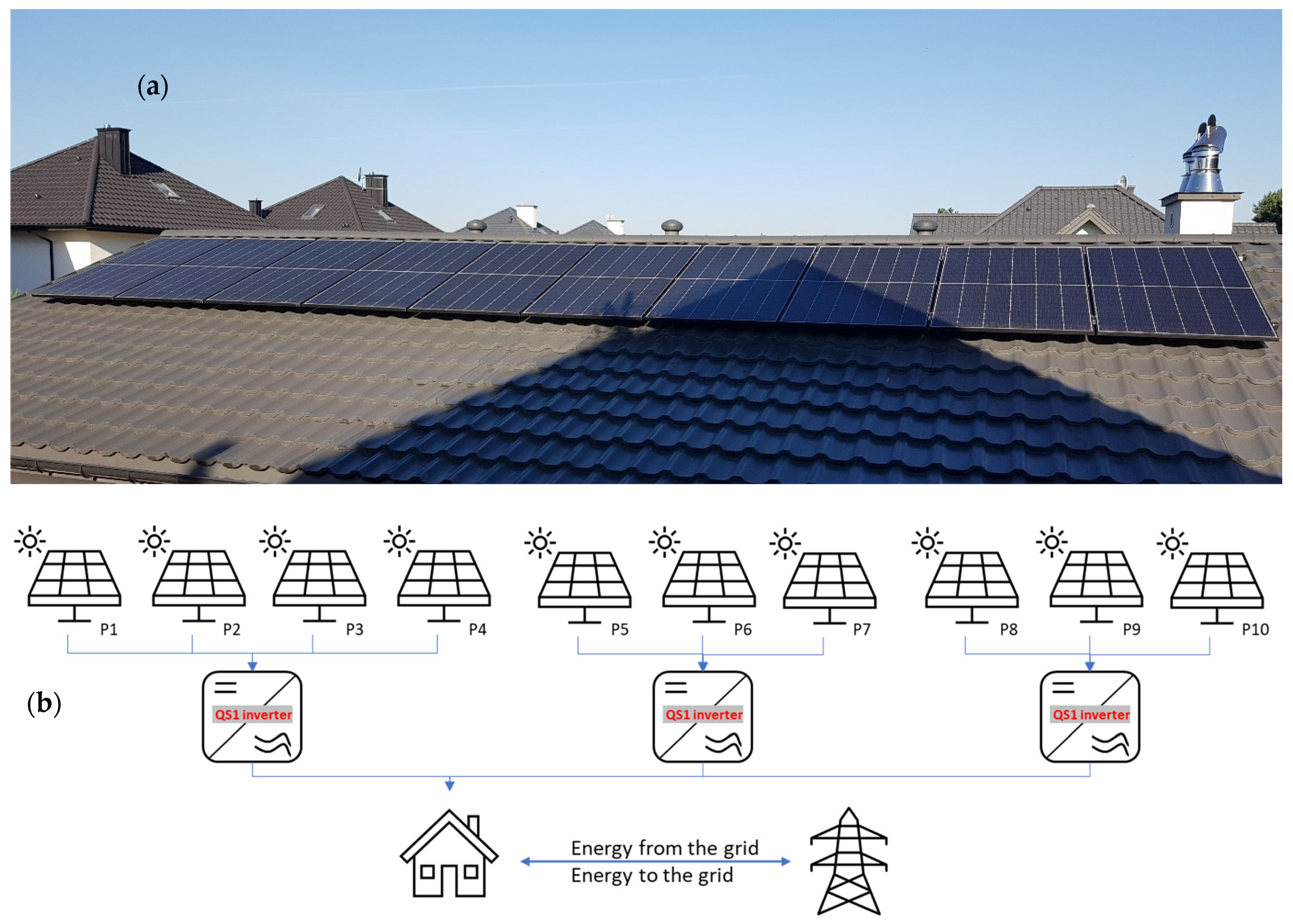
2.1. Research Object

The research object is located in the Piaseczno poviat in the voivodeship Mazowieckie in Poland. This facility is a prosumer micro-installation consisting of 10 Jinko PV panels [15] connected to microinverters. The orientation of the panels is 50° east, 30° inclination to the horizontal plane. This panel setting is based on the configuration of the roof surface (Figure 1), which also affects the temperature of the PV panels (adversely affecting energy productivity [16]). Geographical data of the installation site: 52.03° N, 21.11° E. Properties of PV panels are included in

Table 1. Characteristics of Jinko PV 440 Wp panels (Mono type P). Source: own study based on [15].

Parameter	Unit	Value
Nominal power	Wp	440
Total length	m	1.868
Total width	m	1.134
Panel efficiency ηP	%	20.77
Temperature coefficient of the short-circuit current	%/°C	0.048
Temperature coefficient of the open-circuit voltage	%/°C	−0.28
Temperature coefficient of the power αp	%/°C	−0.35

.

Three QS1 inverters [17] were used with an MPPT voltage range 22–48 V and an operating voltage range 16–55 V. The maximum input voltage is 60 V and the starting voltage is 20 V. Maximum input current is 12 A × 4. Maximum continuous power output is 1400 W. The adjustable output voltage range is 160–278 V. Peak efficiency: 96.5%, nominal MPPT efficiency: 99.5% [17].

The recorded values (from QS1 inverters) of PV energy production unit values in the form of daily sums are shown in Figure 2a, and the differences in the values of energy production between individual panels are included in Figure 2b.

The observed daily differences in the unit energy production between PV panels were below 0.4 kWh/kWp/day. In the winter months, the value was several dozen percent of the total unit energy production. It can be seen during which months the energy production was significantly reduced, and on which panels the shadow (in the morning) influenced this reduction. A detailed analysis is presented in the Results and Discussion section.

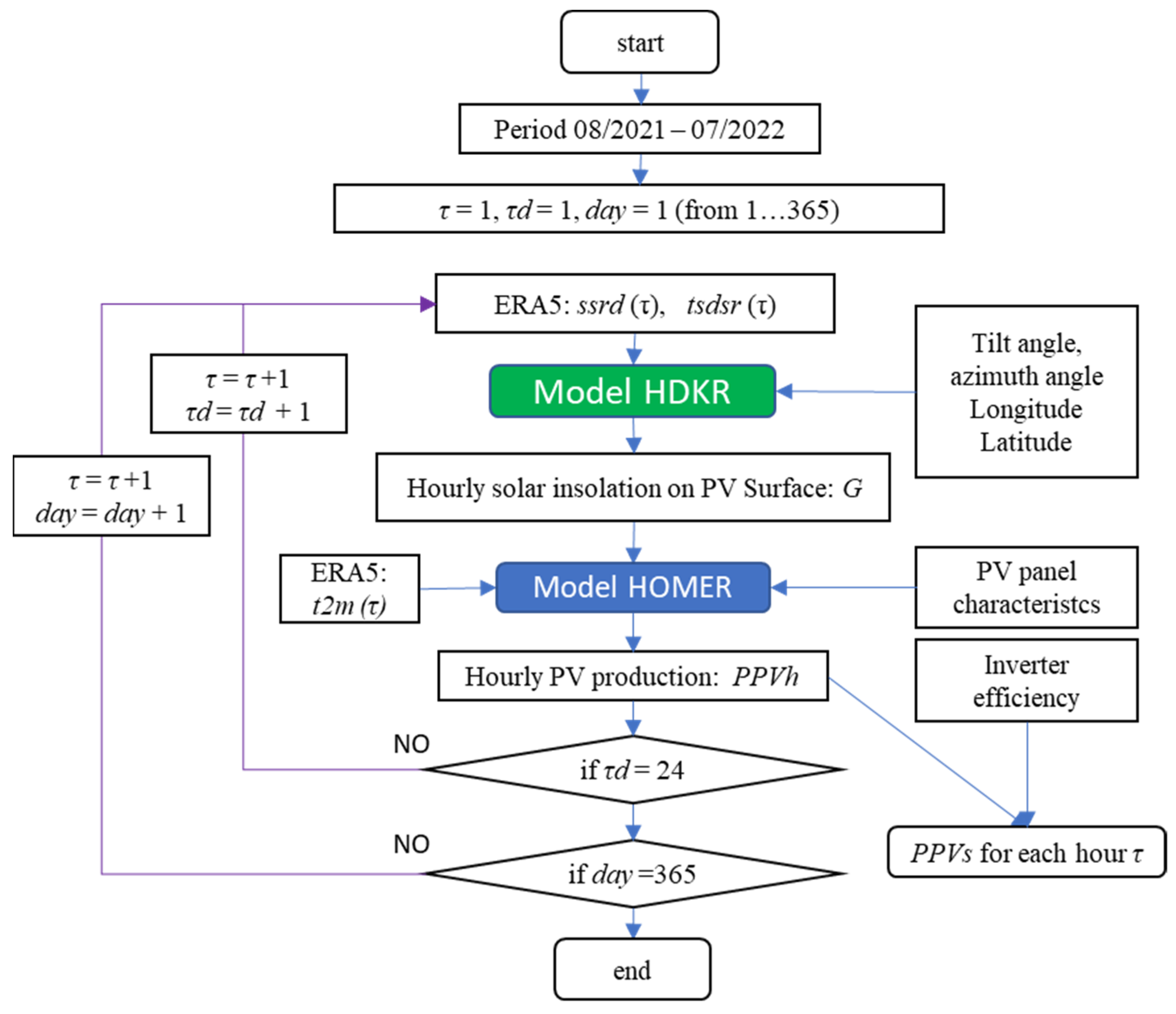
2.2. Solar Radiation Calculation Method

The first step in the calculations was to determine the available solar radiation for PV panels. For this purpose, weather data was collected for the period of operation of the installation (first year; 1 August 2021–31 July 2022). These data were included in the calculations of both the available solar radiation and the energy productivity of the installation (see the figures in Appendix A: Figure A1, Figure A2 and Figure A3). The data retrieved for each hour from ERA5 database [18] are:

• ssrd—surface solar radiation downwards comprises both direct and diffuse solar radiation [19],
• tsdsr—total sky direct solar radiation at surface [20],
• t2m—temperature of air at 2 m above the surface of land [21].

The HDKR model is one of the most accurate models for Central-Eastern European countries [22,23]. It considers the beam, solar radiation (similar to tsdsr), diffuse circumsolar radiation, diffuse isotropic radiation (Gd), diffuse horizontal radiation, and diffuse reflected radiation. The available solar radiation intensity on the plane was determined by the values of the angles γ and β at hour τ calculated using Equation (1) [24,25]. The following ranges of values were included in the analysis: azimuth angle (γ) starting from −90° € up to 90° (W), and tilt (inclination) angle (β) from 0° to 90°.

$$G\left(\tau ,\beta , \gamma \right)=Rb\left(\tau ,\beta , \gamma \right)·\left(tsdsr\left(\tau \right)+Ai\left(\tau \right)·Gd\left(\tau \right)\right)+Rd·\left(1-Ai\left(\tau \right)\right)·\left(1+Rlh\left(\tau ,\beta , \gamma \right)\right)+\rho ·Ro·\left(tsdsr\left(\tau \right)+Gd\left(\tau \right)\right)$$

(1)

where:

• G—available intensity of solar radiation incident on surface dependent on time, tilt angle, and azimuth angle, W/m²
• τ—hour of year
• β—tilt angle, °
• γ—azimuth angle, °
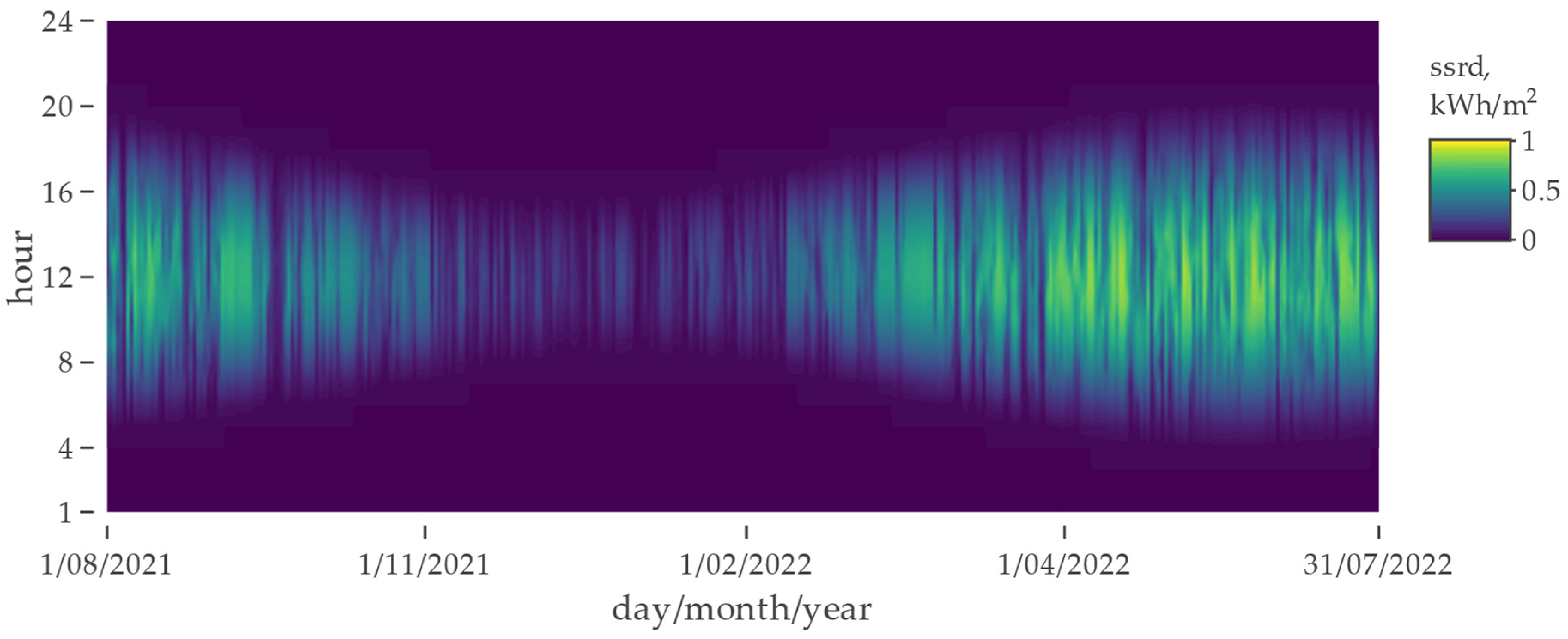
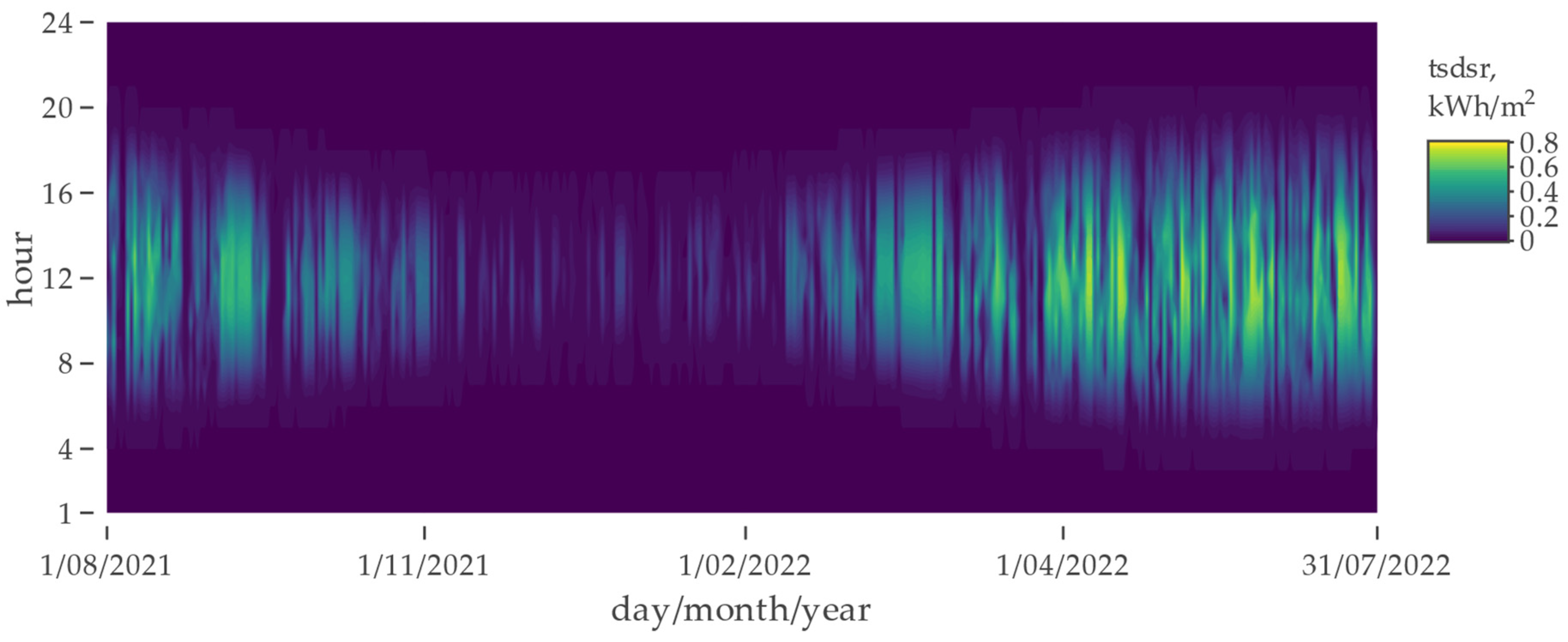
• tsdsr—beam radiation on a horizontal surface, from ERA5 database, please also see Figure A2, W/m²
• Gd—diffuse radiation on a horizontal surface, Equation (2), W/m²
• Ai—anisotropy index,
• Rb—geometric factor of beam radiation on the tilted surface to that on a horizontal surface, see reference [25,26],
• Rd—geometric factor for diffuse radiation, see reference [25,26],
• Rlh—geometric factor for diffuse brightness horizontal radiation, see reference [25,26]
• Ro—geometric factor for diffuse reflected radiation (reflected by surfaces in front of panel surface), see reference [25,26]
• ρ—reflection factor from the ground, see reference [25,26,27].

$$Gd\left(\tau \right)=ssrd\left(\tau \right)-tsdsr\left(\tau \right)$$

(2)

where:

• Gd—diffuse radiation on a horizontal surface, W/m²
• ssrd—direct and diffuse solar radiation, from ERA5 database—Figure A1, W/m²
• tsdsr—total sky direct solar radiation at surface, from ERA5 database—Figure A2, W/m²

The annual insolation value for the plane defined by the values of the γ and β angles was determined according to the following equation [27]:

$$I\left(\beta ,\gamma \right)={{\displaystyle \sum }}_{\tau =1}^{8760 }G\left(\tau ,\beta ,\gamma \right)·\frac{1 h}{1000}$$

(3)

where:

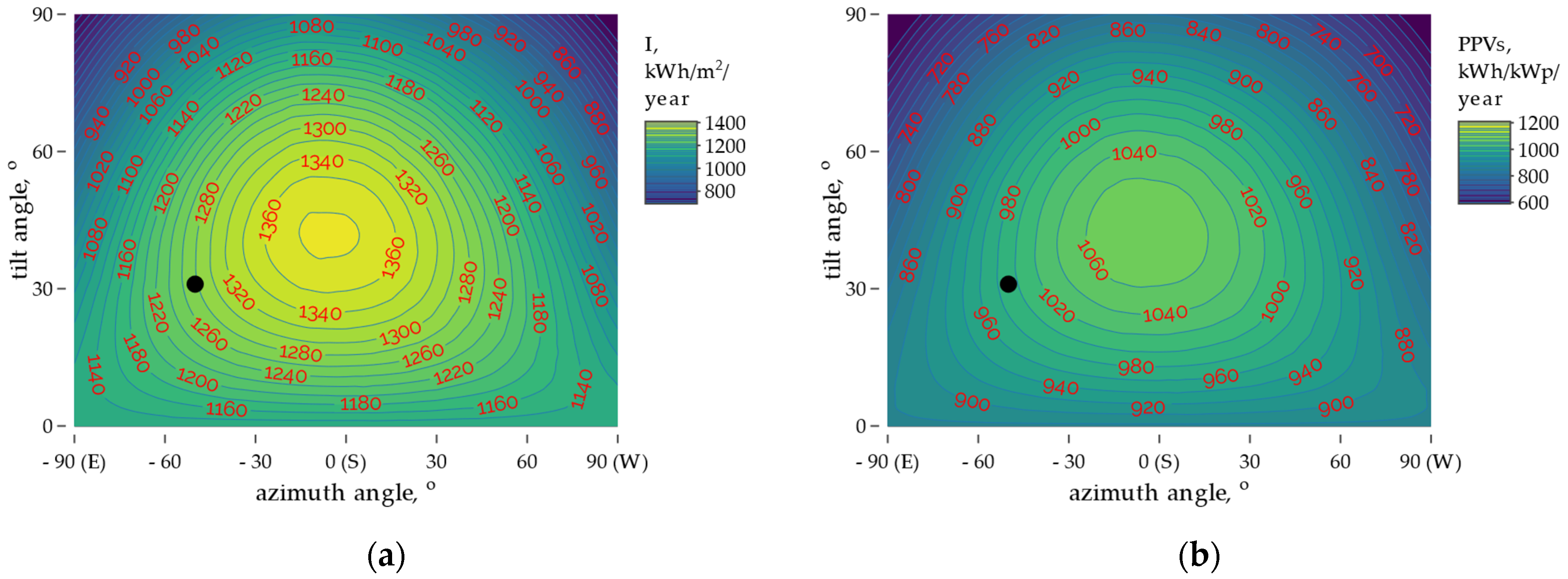
• I—insolation, kWh/m²/year
• G—available intensity of solar radiation incident on surface dependent on time, tilt angle β, and azimuth angle γ, W/m²

2.3. PV Energy Production Calculation Method

The mean (for 10 PV panels) value of hourly PV unit energy production (PPVh) was calculated in accordance with the methodology of the HOMER software [28] and also based on the work of Jordan [29]—Equation (4).

$$PPVh\left(\tau ,\gamma ,\beta \right)=YPV·FPV·\frac{G\left(\tau ,\gamma ,\beta \right)}{GSTC}·\left(1+\alpha p·\left(TC-TSTC\right)\right)·SF\left(year\right)·1h$$

(4)

where:

• PPVh—mean (for 10 PV panels) hourly energy output of photovoltaic panels, kWh/kWp
• YPV—rated capacity of the PV array, which implies that its output power under standard test conditions (1 kWp was used), kW/kWp
• FPV—PV derating factor, 0.90 [27,30]
• G—available intensity of solar radiation incident on surface (for analysed installation: β = 30°, γ = −50° south-east direction) dependent on time, based on ERA5 data and HDKR model, W/m²
• GSTC—incident radiation at Standard Test Conditions, 1 kW/m²
• αp—temperature coefficient of power, based on Jinko PV Data (Table 1: 0.35) %/°C
• TC—PV cell temperature, based on equation included in [31] and ERA5 data (please see Equation (5)), °C
• TSTC—PV cell temperature under standard test conditions (25 °C)
• SF—Shadow factor of PV panels—Equation (6)

PV cell temperature for each hour was calculated based on Equation (5).

$$TC\left(\tau ,\gamma ,\beta \right)=t2m\left(\tau \right)+G\left(\tau ,\gamma ,\beta \right)·\frac{TC.NOCT-Ta.NOCT}{G.NOCT}·\left(1-\frac{\eta p}{ta}\right)$$

(5)

where:

• TC—PV cell temperature, °C
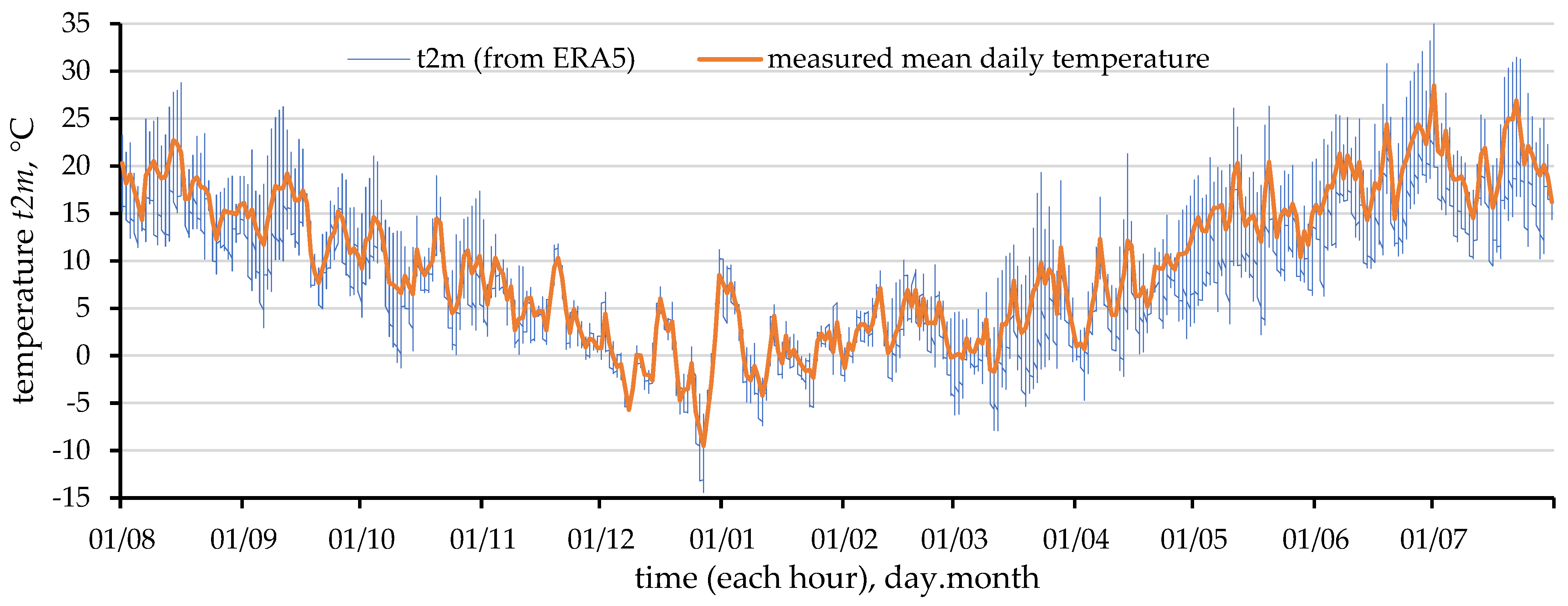
• t2m—temperature of air at 2 m above the surface of land, from ERA5 database, please also see Figure A3, °C
• TC.NOCT—nominal operating cell temperature (45 °C [15]), °C
• Ta.NOCT—ambient temperature at which the NOCT is defined (20 °C [15]), °C
• G.NOCT—solar radiation at which the NOCT is defined (0.8 kW/m² [15,27]), W/m²
• ηp—panel efficiency (from Table 1),
• ta—coefficient of transmittance and absorptance, 0.9 [25]

The shadow factor of PV panels was calculated based on the following equation:

$$SF\left(year\right)=\frac{min2P\left(year\right)}{PPV6m\left(year\right)}$$

(6)

where:

• SF—shadow factor of PV panels
• min2P—mean measured value of two PV panels with minimum yearly energy production, kWh/kWp/year
• PPV6m—mean measured value of PV energy production from 6 PV panels (with mean energy production from 10 PV panels), kWh/kWp/year

The daily unit electricity production ($PPVs$) in a photovoltaic installation was calculated by Equation (7).

$$PPVs\left(day,\gamma ,\beta \right)={{\displaystyle \sum }}_{\tau d=1}^{24}PPVh\left(\tau d,\gamma ,\beta ,day\right)·{\eta }_{inverter}$$

(7)

where:

• PPVs—theoretical daily unit electricity production in PV installation in, kWh/kWp/day
• PPVh—hourly energy output of photovoltaic panels, kWh/kWp/hour
• η_inverter—inverter efficiency, %
• τd—day hour, extracted from hour of year (τ)
• day—the following day of first PV installation operational year

The simplified algorithm of calculation for daily unit electricity production ($PPVs$) is presented in Figure 3.

The comparison of daily and monthly calculated values of PV energy production with the measured values was made according to the following equations for RSME [32], d. and for rMBE.

$$RSME\left(PPV\right)=\sqrt{\frac{{{\displaystyle \sum }}_1^n{\left(PPVm\left(day\right)-PPVs\left(day,\gamma =-50°,\beta =30°\right)\right)}^2}{n}}$$

(8)

where:

• n—total number of daily observations, whole year, n = 365
• day—day of calculation
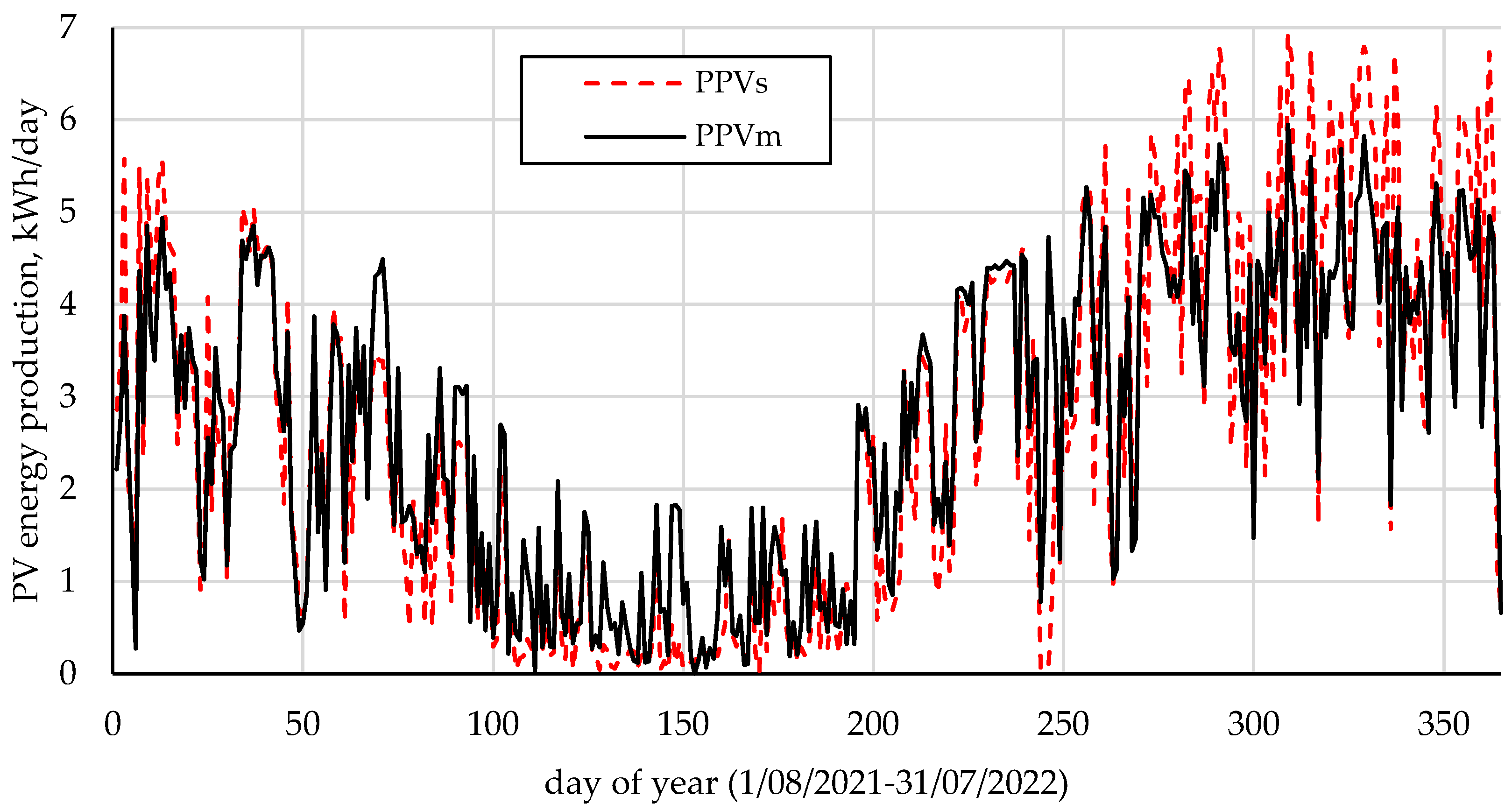
• PPVm—measured value of daily PV energy production, kWh/kWp/day
• PPVs—simulated value of daily PV energy production, kWh/kWp/day

The percentage difference between the simulation results and the measured values was calculated according to Equation (9).

$$d.\left(month\right)=\frac{PPVs\left(month, \gamma =-50°,\beta =30°\right)-PPVm\left(month\right)}{PPVm\left(month\right)}$$

(9)

where:

• d.—percentage difference between simulated (from model) and measured results (PV energy production), %
• month—month of calculation

The comparison of the daily and monthly (analogically determined as for the daily) calculated values of PV energy production with the measured values was made according to the following equation on relative mean bias error (rMBE) [33]:

$$rMBE=\frac{{{\displaystyle \sum }}_{day}\left(PPVs\left(day,\gamma =-50°,\beta =30°\right)-PPVm\left(day\right)\right)}{{{\displaystyle \sum }}_{day}PPVm\left(day\right)}$$

(10)

3. Results and Discussion

3.1. Insolation and Theoretical Productivity Simulation Results

Based on the HDKR method and ERA5 weather data, access to solar radiation in the form of insolation was estimated (as a function of azimuth and tilt angle, Equation (3))—Figure 4a. Figure 4b contains the results in the form of estimated electricity production from PV panels.

In the first analyzed year of installation (August 2021–July 2022), the horizontal insolation value (yearly sum of ssrd) reached 1126 kWh/m2/year, which is 1% higher than the average annual value of horizontal insolation for 2001–2021 (1111 kWh/m2/year) [18]. The maximum available insolation can be observed for the south-facing plane with an inclination of approximately 40° and is approximately 1380 kWh/m²/year. The configuration of the location of the analyzed PV installation results in the availability of insolation of 1275 kWh/m²/year.

The annual energy production for panels located on the horizontal plane would be 880 kWh/kWp/year. For the analyzed PV installation, this value was 995 kWh/kWp/year, which is 80 kWh/kWp/year lower than for the configuration causing the highest theoretical productivity of the PV installation (1075 kWh/kWp/year for the south-oriented PV panel and tilt angle 40°).

Determination of the shading factor.

The cumulative values of differences in the production of individual PV panels are shown in Figure 5. They were used to determine the shading coefficient SF (Equation (6)).

During the first year of operation of the PV installation, the P8 panel produced 3.8% (16.4 kWh/year, i.e., 37.3 kWh/kWp/year) less energy than the calculated average value (969.1 kWh/kWp/year) for all PV panels in the installation. On the other hand, the P3 panel produced 3.4% more energy than the above-mentioned average value. In the case of five panels, the difference between the average value of energy produced and that which was measured for a given panel did not exceed 2%. Significantly, the largest difference, calculated between the deviations calculated from the mean value, was noted for the P7 panel (+2.6% above the mean) compared to the P8 panel (−3.8%). In the case of the P8 panel, the reason for the lower-than-average value of energy production could be (compared to other panels in the installation) partial shading, especially in the morning (please also see Figure 2). However, an adjacent panel (P7) produced more energy than the calculated average.

Data on the energy production from the two panels with the lowest energy production (i.e., P8 and P9) were used to determine the min2P value. The average production value of 6 panels with an average energy production of 10 is the value of PPV6m. Thanks to the determination of these values, the value of the SF index equal to 0.98 for the first year was calculated.

3.2. Comparison of Measured and Simulated Data of PV Energy Productivity

A comparison of the daily values of energy production from PV installations (measured and simulated data) is included in Figure 6.

In the spring–summer period, the measured daily energy production values were higher than the calculated values in the model. On the other hand, in the winter period, the energy production values from the model were higher than those measured. One of the reasons for the lower than expected energy production value in the winter period could be snow (due to the low value tilt angle i.e., lower than 40°), or the icing or shading of the PV panels.

The values presented in Figure 6 have been aggregated to monthly sums—Figure 7.

The highest percentage difference was achieved for December 2021 (139.3% higher energy production according to the model than according to the measurement). This result is similar to that observed for the Leki installation [27]. Differences below 10% were recorded for August, September, March, and May. In total, the unit annual energy production amounted to 986.9 kWh/kWp as the result of the calculations (presented methodology) and 969.1 kWh/kWp as the measured value (inverters). This means that the value of energy production calculated according to the presented methodology is 1.8% higher than the measured value.

The RSME value is 0.79 kWh/kWp/day with an average daily energy production value of 2.66 kWh/kWp/day. The rMBE value is 0.018.

4. Conclusions

The operation of an installation consisting of 10 photovoltaic panels over a period of one year in the conditions of central Poland was analyzed. Discrepancies in the amount of energy production between individual photovoltaic panels were shown, this being up to 3.8% per year, i.e., 37.3 kWh/kWp/year). The solar radiation availability was calculated based on the HDKR model and ERA5 weather data. Next, the theoretical productivity of the photovoltaic installation was calculated on an hourly scale and aggregated to a daily scale. The obtained results in the form of theoretical values and practical values were compared, and the largest discrepancies in the percentage scale were achieved for December. The shading coefficient was also determined based on the difference in energy production by PV panels.

Based on the research, it can be concluded that the HOMER method works well for the installation of single-sided photovoltaic panels with microinverters (difference in the annual period of less than 2%, rMBE value 0.018). The future direction of research will be:

• a detailed analysis of the influence of the shading of the installation on the productivity of individual panels and the determination of their representativeness,
• economic analyses—comparison between PV installation with standard inverter and with micro-inverters for households PV.

References

1. Milosavljević, D.D.; Kevkić, T.S.; Jovanović, S.J. Review and validation of photovoltaic solar simulation tools/software based on case study. Open Phys. 2022, 20, 431–451. [Google Scholar] [CrossRef]
2. Barco Jiménez, J.; Pantoja, A.; Caicedo Bravo, E. Optimal sizing of a grid-connected microgrid and operation validation using HOMER Pro and DIgSILENT. Sci. Tech. 2022, 27, 28–34. [Google Scholar]
3. Bentouba, S.; Bourouis, M.; Zioui, N.; Pirashanthan, A.; Velauthapillai, D. Performance assessment of a 20 MW photovoltaic power plant in a hot climate using real data and simulation tools. Energy Rep. 2021, 7, 7297–7314. [Google Scholar] [CrossRef]
4. Roberts, J.; Cassula, A.; Freire, J.; Prado, P. Simulation and Validation Of Photovoltaic System Performance Models. In Proceedings of the XI Latin-American Congress on Electricity Generation and Transmission–CLAGTEE 2015, Sao Paulo, Brazil, 8–11 November 2015. [Google Scholar]
5. Barros, L.A.M.; Tanta, M.; Sousa, T.J.C.; Afonso, J.L.; Pinto, J.G. New Multifunctional Isolated Microinverter with Integrated Energy Storage System for PV Applications. Energies 2020, 13, 4016. [Google Scholar] [CrossRef]
6. Tariq, M.S.; Butt, S.A.; Khan, H.A. Impact of module and inverter failures on the performance of central-, string-, and micro-inverter PV systems. Microelectron. Reliab. 2018, 88–90, 1042–1046. [Google Scholar] [CrossRef]
7. Gagrica, O.; Marzec, M.; Uhl, T. Comparison of reliability impacts of two active power curtailment methods for PV micro-inverters. Microelectron. Reliab. 2016, 58, 133–140. [Google Scholar] [CrossRef]
8. Chub, A.; Vinnikov, D.; Stepenko, S.; Liivik, E.; Blaabjerg, F. Photovoltaic Energy Yield Improvement in Two-Stage Solar Microinverters. Energies 2019, 12, 3774. [Google Scholar] [CrossRef] [Green Version]
9. Elanchezhian, P.; Chinnaiyan, V.K. Modeling and Simulation of High-Efficiency Interleaved Flyback Micro-inverter For Photovoltaic Applications. Mater. Today Proc. 2017, 4, 10417–10421. [Google Scholar] [CrossRef]
10. Sinapis, K.; Litjens, G.B.M.A.; van den Donker, M.N.; Folkerts, W.; van Sark, W. Outdoor characterization and comparison of string and MLPE under clear and partially shaded conditions. Energy Sci. Eng. 2015, 3, 510–519. [Google Scholar] [CrossRef]
11. Sinapis, K.; Tzikas, C.; Litjens, G.; van den Donker, M.; Folkerts, W.; van Sark, W.G.J.H.M.; Smets, A. A comprehensive study on partial shading response of c-Si modules and yield modeling of string inverter and module level power electronics. Sol. Energy 2016, 135, 731–741. [Google Scholar] [CrossRef] [Green Version]
12. Sher, H.A.; Addoweesh, K.E. Micro-inverters—Promising solutions in solar photovoltaics. Energy Sustain. Dev. 2012, 16, 389–400. [Google Scholar] [CrossRef]
13. Kouro, S.; Leon, J.I.; Vinnikov, D.; Franquelo, L.G. Grid-Connected Photovoltaic Systems: An Overview of Recent Research and Emerging PV Converter Technology. IEEE Ind. Electron. Mag. 2015, 9, 47–61. [Google Scholar] [CrossRef]
14. European Centre for Medium-Range Weather Forecasts (ECMWF) ERA5. Available online: https://confluence.ecmwf.int/display/CUSF/ERA5+hourly+data+on+single+level+and+ERA5+hourly+on+pressure+levels+available+again+from+the+CDS?src=contextnavpagetreemode (accessed on 28 August 2022).
15. Jinko. PV Jinko 440 Wp Monofacial. Available online: https://sklep.enexon.pl/amfile/file/download/file/268991/product/99172/ (accessed on 26 August 2022).
16. Canales, F.A.; Jadwiszczak, P.; Jurasz, J.; Wdowikowski, M.; Ciapała, B.; Kaźmierczak, B. The impact of long-term changes in air temperature on renewable energy in Poland. Sci. Total Environ. 2020, 729, 138965. [Google Scholar] [CrossRef] [PubMed]
17. APSystems. Micro–Inwerter QS1. Available online: https://b2b.eltech.net.pl/pl/product/83977,micro-inwerter-qs1 (accessed on 31 August 2022).
18. Copernicus. ERA5 Hourly Data on Single Levels from 1979 to Present. Available online: https://cds.climate.copernicus.eu/cdsapp#!/dataset/reanalysis-era5-single-levels?tab=overview (accessed on 16 March 2022).
19. ECMWF. Surface Solar Radiation Downwards. Available online: https://apps.ecmwf.int/codes/grib/param-db?id=169 (accessed on 3 September 2022).
20. ECMWF. Total Sky Direct Solar Radiation at Surface (fdir). Available online: https://apps.ecmwf.int/codes/grib/param-db?id=228021 (accessed on 3 September 2022).
21. ECMWF. 2 Metre Temperature. Available online: https://apps.ecmwf.int/codes/grib/param-db?id=167 (accessed on 3 September 2022).
22. Karlsson, J. Windows—Optical Performance and Energy Efficiency; Acta Universitatis Upsaliensis: Uppsala, Sweden, 2001. [Google Scholar]
23. Chwieduk, D.; Chwieduk, M. Determination of the Energy Performance of a Solar Low Energy House with Regard to Aspects of Energy Efficiency and Smartness of the House. Energies 2020, 13, 3232. [Google Scholar] [CrossRef]
24. Chwieduk, D.A. Recommendation on modelling of solar energy incident on a building envelope. Renew. Energy 2009, 34, 736–741. [Google Scholar] [CrossRef]
25. Duffie, J.A.; Beckman, W.A. Solar Engineering of Thermal Processes; John Wiley & Sons: Hoboken, NJ, USA, 2006. [Google Scholar]
26. Olek, M.; Olczak, P.; Kryzia, D. The sizes of Flat Plate and Evacuated Tube Collectors with Heat Pipe area as a function of the share of solar system in the heat demand. In Proceedings of the 1st International Conference on the Sustainable Energy and Environment Development (SEED 2016), Kraków, Poland, 17–19 May 2016; Volume 10, p. 00139. [Google Scholar]
27. Olczak, P.; Komorowska, A. An adjustable mounting rack or an additional PV panel? Cost and environmental analysis of a photovoltaic installation on a household: A case study in Poland. Sustain. Energy Technol. Assess. 2021, 47, 101496. [Google Scholar] [CrossRef]
28. HOMER. Homer Energy. Available online: https://www.homerenergy.com/index.html (accessed on 20 October 2020).
29. Jordan, D.C.; Deceglie, M.G.; Kurtz, S.R. PV Degradation Methodology Comparison—A Basis for a Standard. In Proceedings of the 2016 IEEE 43rd Photovoltaic Specialists Conference (PVSC), Portland, OR, USA, 5–10 June 2016. [Google Scholar]
30. Al Garni, H.Z.; Awasthi, A.; Ramli, M.A.M. Optimal design and analysis of grid-connected photovoltaic under different tracking systems using HOMER. Energy Convers. Manag. 2018, 155, 42–57. [Google Scholar] [CrossRef]
31. Olczak, P.; Żelazna, A.; Matuszewska, D.; Olek, M. The “My Electricity” Program as One of the Ways to Reduce CO2 Emissions in Poland. Energies 2021, 14, 7679. [Google Scholar] [CrossRef]
32. Shukla, K.N.; Rangnekar, S.; Sudhakar, K. Comparative study of isotropic and anisotropic sky models to estimate solar radiation incident on tilted surface: A case study for Bhopal, India. Energy Rep. 2015, 1, 96–103. [Google Scholar] [CrossRef] [Green Version]
33. O’Sullivan, B.; Chalhoub-Deville, M. Language Testing for Migrants: Co-Constructing Validation. Lang. Assess. Q. 2021, 18, 547–557. [Google Scholar] [CrossRef]
34. IMGW. Temperature for Warszawa Filtrowo Weather Station. Available online: https://danepubliczne.imgw.pl/data/dane_pomiarowo_obserwacyjne/dane_meteorologiczne/dobowe/klimat/ (accessed on 27 September 2022).
Figure 1. (a) Microinverter Photovoltaic Microinstallation in Masovian Region—Poland. From left P1 to right up to P10 number of PV panel; (b) PV panels configuration scheme.
Energies 15 07582 g001
Figure 2. (a) Daily sum energy production from 10 PV panels; (b) difference between daily PV energy production and 10 panels daily mean energy production for the first operational year: 1 August 2021–31 July 2022. Source: own study.
Energies 15 07582 g002
Figure 3. Simplified algorithm of calculation for PV energy production for each hour.
Energies 15 07582 g003
Figure 4. Results of calculation for the first operational year: (a) Insolation as a function of azimuth and tilt angle for the first operational year, based on HDKR model and ERA5 data; (b) PV energy productivity (from model: PPVs, based on Equation (7)) as a function of azimuth and tilt angle, based on HDKR model, ERA5 data, and HOMER method; ●—value for existing PV installation.
Energies 15 07582 g004
Figure 5. Comparison of energy production from 10 PV panels for the first operational year, August 2021–July 2022.
Energies 15 07582 g005
Figure 6. Comparison of measured (PPVm) and simulated (from model: PPVs, Equation (7)) daily results of photovoltaic energy productivity for the first operational year.
Energies 15 07582 g006
Figure 7. Comparison of simulation and measured monthly results of energy photovoltaic productivity for the first operational year August 2021–July 2022. d.—percentage difference between simulated (from model, PPVs) and measured (PPVm) energy production results.
Energies 15 07582 g007