A Review of Laboratory and Numerical Techniques to Simulate Turbulent Flows

Abstract

Turbulence is still an unsolved issue with enormous implications in several fields, from the turbulent wakes on moving objects to the accumulation of heat in the built environment or the optimization of the performances of heat exchangers or mixers. This review deals with the techniques and trends in turbulent flow simulations, which can be achieved through both laboratory and numerical modeling. As a matter of fact, even if the term “experiment” is commonly employed for laboratory techniques and the term “simulation” for numerical techniques, both the laboratory and numerical techniques try to simulate the real-world turbulent flows performing experiments under controlled conditions. The main target of this paper is to provide an overview of laboratory and numerical techniques to investigate turbulent flows, useful for the research and technical community also involved in the energy field (often non-specialist of turbulent flow investigations), highlighting the advantages and disadvantages of the main techniques, as well as their main fields of application, and also to highlight the trends of the above mentioned methodologies via bibliometric analysis. In this way, the reader can select the proper technique for the specific case of interest and use the quoted bibliography as a more detailed guide. As a consequence of this target, a limitation of this review is that the deepening of the single techniques is not provided. Moreover, even though the experimental and numerical techniques presented in this review are virtually applicable to any type of turbulent flow, given their variety in the very broad field of energy research, the examples presented and discussed in this work will be limited to single-phase subsonic flows of Newtonian fluids. The main result from the bibliometric analysis shows that, as of 2021, a 3:1 ratio of numerical simulations over laboratory experiments emerges from the analysis, which clearly shows a projected dominant trend of the former technique in the field of turbulence. Nonetheless, the main result from the discussion of advantages and disadvantages of both the techniques confirms that each of them has peculiar strengths and weaknesses and that both approaches are still indispensable, with different but complementary purposes.

1. Introduction

Turbulence can be defined in several ways but all of them in some way remark that a turbulent flow is as a state of a fluid flow which is very irregular in time and in space: one of the ascertained consequences of this irregularity is that turbulence is not deterministic, i.e., it is not completely predictable from some initial or boundary conditions, as an infinitesimal change in those initial conditions produces a finite change in the following motion. On the opposite, a laminar flow is regular in time and in space and, given some initial or boundary conditions, predictable, with the same degree of approximation of the given initial conditions: so, in other words, it is deterministic (see, among the others, Tennekes and Lumley [1], Falkovich et al. [2], and Davidson [3]). Even if several descriptions of turbulence features have been given during the centuries, starting from Leonardo da Vinci’s descriptions, (Marusic and Broomhall [4]), a definitive definition of turbulence, taking into account all its characteristics, is still difficult to be achieved, even if some common features can be identified, such as fluctuating velocities, a multiscale behavior, the presence of organized structures in the form of vortex filaments and of stagnation points, just to recall the most common (Davidson [3]). The most relevant consequence in everyday life of this lack of a complete comprehension of turbulent flows is that, after almost one and a half centuries from the seminal experiments of Reynolds (Reynolds [5], but see also the critical review of Jackson and Launder [6]) and despite the fact that the governing equations (the Navier–Stokes equations, see Equation (1) below) have been known since the XIX century, a complete understanding of turbulent flows is far from being achieved, leaving turbulence as an “undefinable concept”, according to Frisch [7], and as the only unresolved field of classical Mechanics. This often-mentioned sentence by Sir Horace Lamb (see, e.g., Goldstein and Hultgren [8]) can give an idea of the difficulties encountered in the field of turbulence: “I am an old man now, and when I die and go to Heaven there are two matters on which I hope enlightenment. One is quantum electro-dynamics and the other is turbulence. About the former, I am really rather optimistic”.

This has enormous consequences in practically every field of human life, as turbulent flows are present almost everywhere and at a broad range of length scales, from ${10}^{23}$ m in galaxies and ${10}^7$ m in the Earth’s atmosphere or ${10}^3$ m in clouds, to ${10}^{-2}$ m in soap films or ${10}^{-5}$ m in liquid crystal flows. Consequently, this lack of understanding of turbulent flows is possibly the most serious obstacle to reach a systematic description of many important engineering and environmental phenomena. Only to quote some, the reduction in energy losses in the movement of cars (Ferraris et al. [9], Palanivendhan et al. [10], Igali et al. [11], Kurec and Piechna [12]) trains (Wang et al. [13] and [14], Zhang et al. [15]) and aircrafts (Bollt and Bewley [16], Varshney et al. [17], Miller et al. [18]), the improvement in the efficiency of engines (Kazmouz et al. [19], Balmelli et al. [20], Krastev and Di Ilio [21]) and the reduction in their noise (Zhong et al. [22], Polacsek et al. [23], Jun et al. [24]), the dispersion of pollutants released in the atmosphere (Bellini et al. [25], Huertas et al. [26], Defforge et al. [27], Di Bernardino et al. [28]) or in the ocean (Liang et al. [29], Chen et al. [30], Lee et al. [31]), the weather forecasts (Chiniforoush et al. [32], Tsiringakis et al. [33], Verbitsky and Khodzinskaya [34]), the atmospheric boundary layers (Di Bernardino et al. [35], Lu and Li [36], Tkachenko et al. [37]), Barbarosa et al. [38]),the mixing and combustion in chemical reactors (Soto et al. [39], Janoszek and Masny [40], Mularski and Modliński [41]), the optimization of turbines (Pacciani et al. [42], Duthè et al. [43], Yang et al. [44]), the study of the air flowing through the lungs (Wu et al. [45], Rajendran and Banerjee [46], Singh et al. [47]), the non-equilibrium turbulent flows (Bourguet et al. [48], Cafiero and Vassilicos [49], Lapsa and Daham [50]), the particle transport in geophysical flows (He et al. [51], Berk and Coletti [52], Boffetta et al. [53]), the analysis of rough boundary layers (Clauser [54], Piomelli [55], Ohya [56], Otten III and van Kuren [57], Kornilov and Boiko [58]), the optimization of heat transfer (Jiao et al. [59], Grądziel et al. [60], Prończuk and Krzanowska [61], Ngwa et al. [62]), and the supersonic flows (Kovasznay [63], Volov et al. [64], Li et al. [65]), etc.

As stated before, non-reacting adiabatic Newtonian fluid flows are described by the Navier–Stokes equations together with the mass conservation equation:

$$\begin{array}{c}\hfill \left\{\begin{array}{c}{\displaystyle \frac{D{u}_i}{Dt}}=a_i=f_i-{\displaystyle \frac{1}{\rho }}{\displaystyle \frac{\partial p}{\partial x_i}}+\nu \left({\displaystyle \frac{{\partial }^2{u}_i}{\partial x_j\partial x_j}}+{\displaystyle \frac{1}{3}}{\displaystyle \frac{\partial }{\partial x_i}}{\displaystyle \frac{\partial u_j}{\partial x_j}}\right)\hfill \\ {\displaystyle \frac{D\rho }{Dt}}+\rho {\displaystyle \frac{\partial u_j}{\partial x_j}}=0\hfill \end{array}\right.\end{array}$$

(1)

where $D/Dt$ denotes the Lagrangian (or total or material) derivative, $u_i$ is the fluid velocity, $a_i$ is the fluid acceleration, $f_i$ is the forcing, $\partial p/\partial x_i$ is the pressure gradient, $\rho$ is the fluid density, $\nu$ is the fluid kinematic viscosity, ${\partial }^2{u}_i/\partial x_j\partial x_j$ is the velocity Laplacian and $\partial u_j/\partial x_j$ is the velocity divergence. The acceleration of a fluid is the Lagrangian derivative of the velocity (Equation (2)) and so it is by its nature a Lagrangian quantity: this implies it is directly measurable by Lagrangian measurement techniques only:

$$a_i=\frac{D{u}_i}{Dt}=\frac{\partial u_i}{\partial t}+u_j\frac{\partial u_i}{\partial x_j}=\frac{\partial u_i}{\partial t}+\frac{\partial u_i}{\partial x_j}{u}_i$$

(2)

Anyway, it can be extracted by the sum of its two components, the local acceleration (the partial temporal derivative of velocity) and the advective acceleration (or transport terms, i.e., the partial spatial derivatives of the velocity times the transport velocity; see Equation (2)); however, the data from laboratory (and numerical) simulations are necessarily discrete, so this implies an approximation, because the partial derivatives must be approximated as finite differences.

As above stated, fluid flows are not always, in general, turbulent: they become turbulent when the Reynolds number Re, the ratio between inertial and viscous forces or, as it is usually represented, the ratio of a typical flow velocity U times a typical flow length-scale L divided by the fluid kinematic viscosity $\nu$, is high enough, i.e., larger than a certain critical value, depending on the particular phenomenon under investigation.

$$Re=\frac{UL}{\nu }$$

(3)

As $Re$ tends to infinite, the so-called fully developed turbulence is reached, where the statistics of the velocity fluctuations are independent of Re itself, the effect of viscous forces is negligible and nonlinearity dominates the flow: a statistical description over a broad range of data is so necessary to describe this complicated and irregular behavior.

However, is turbulence a random phenomenon? For many decades the answer to this question was positive and turbulence was studied only from a statistical point of view; however, it has been shown that the statistics of particle pair dispersion in turbulent flows (proportional to the third power of time) are different from the ones in Brownian motion (random walk) (Ottino [66]), providing an (optimistic?) perspective for a future general comprehension.

In any case, currently the turbulent flows have to be investigated through the statistical analysis of large data-sets, which can be obtained thanks to the increased performance of up-to-date numerical and laboratory simulation and measurement techniques, which hold the potentiality to allow the scientific community to gain new insights and knowledge and go toward a deeper understanding of turbulent flows, with a consequent energy consumption optimization in all the turbulence related fields, and helping to reduce the related pollution as well.

As a consequence, the two main targets of this paper are:

• To provide an overview of the present laboratory and numerical techniques to investigate turbulent flows useful for the research and technical community involved in the energy field (often non-specialist of turbulent flow investigations), highlighting advantages and disadvantages of the main techniques, as well as their main fields of application, in order to help the reader in selecting the proper technique for the specific case of interest and then, following the related bibliography, in deepening the selected one; to the best of the authors’ knowledge, this is the first review paper with these features. As a consequence of this target, the limitations of this review are twofold: on one hand the details of each single technique cannot be provided and, on the other hand, even though the experimental and numerical techniques presented in this review are virtually applicable to any type of turbulent flow, given the numerous features and characteristics encountered in the very broad field of energy research, the examples presented and discussed in this work is limited to single-phase subsonic flows of Newtonian fluids.
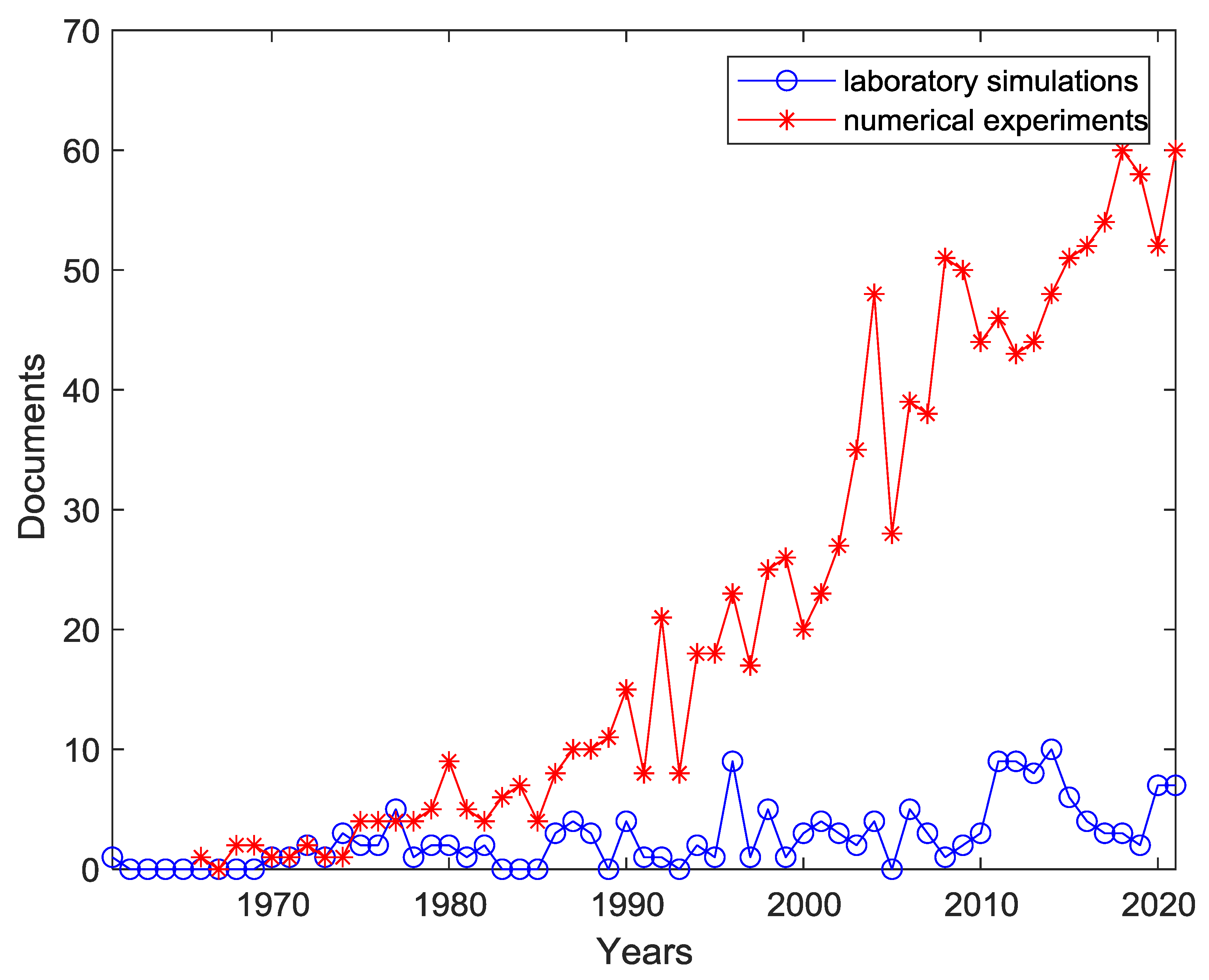
• To highlight the trends of the above mentioned two methodologies in the investigations of turbulent flows.

Moreover, at the end of the paper we also provide a taxonomic analysis of the commonly employed language in turbulent related fields in order to contribute to a revision of the commonly employed language. This because, even if the term “experiment” is commonly employed for laboratory techniques and the term “simulation” for the numerical techniques, both the laboratory and numerical techniques try to simulate the real-world turbulent flows performing experiments under controlled conditions, so the community could go beyond this sharp separation between “laboratory experiments” and “numerical simulations”. The following of this paper is organized as follows: in Section 2, a review of the technique for the laboratory simulation of turbulent flows is given; Section 3 deals with a review of the technique for the numerical simulation of turbulent flows; in Section 4, advantages and disadvantages of laboratory and numerical simulations are given, as well as the trends of techniques in the investigations of turbulent flows, also through a bibliometric analysis, to then face the topic of the meaning of words such as “simulation” and “experiment” in the contemporary field of turbulent flow investigation, to eventually draw conclusions and final remarks.

2. Laboratory Simulations of Turbulent Flows

The first modern scientific investigations on turbulence were made via laboratory experiments, starting from the above quoted seminal experiments of Reynolds [5] and from the first papers citing laboratory experiments on turbulence and indexed on Scopus by Mackenzie and Honaman [67] and of Tice [68], as for many decades this was the only available way, except, of course, the direct observation of real life phenomena which had the obvious defect to not be repeatable. Nowadays, even if the increasing computational capabilities of computers has made numerical simulations the most common way of investigating turbulent flows (see Section 4), laboratory experiments are still indispensable, because they are needed to validate and calibrate novel codes and models for numerical simulations, because it is easier and less time-consuming to reach high Reynolds numbers in the laboratory (see, e.g., Frisch [7]) and, last but not least, because they are still the most affordable way to reproduce novel phenomena involving turbulent flows and not investigated before.

The first way to investigate turbulent flows in the laboratory was by means of flow visualization and observation performed by the scientist, which was soon replaced and/or sustained by quantitative measurements via physical probes inserted into the flow (the first measurements of this kind reported on papers indexed in Scopus are the Pitot tube ones by Bellet [69]). The drawback of physical probes is that they are intrusive, i.e., alter the flow they are supposed to measure, and pointwise, i.e., they take measures in a single point of the flow. This means that many experiments are needed to obtain a two-dimensional (2D) or three-dimensional (3D) representation of the flow field. Otherwise, racks of probes can be employed, but of course the more the probes are, the more the flow to observe is altered. To overcome the first drawback, non-intrusive or quasi non-intrusive (or minimally intrusive) techniques have been developed, while to overcome the second one planar and volumetric techniques have been designed. On the other hand, usually physical probes can achieve, with equal cost, higher temporal frequencies than non-intrusive techniques.

In the following, Section 2.1 is devoted to the intrusive techniques, and Section 2.2 to the non-intrusive and quasi non-intrusive (or minimally intrusive) techniques employed to perform measurements in turbulent flows, with a particular attention to the techniques based on digital image analysis (DIA), while Section 2.3 details a brief discussion on the accuracy of the velocity measurement provided by the main techniques.

2.1. Intrusive Techniques

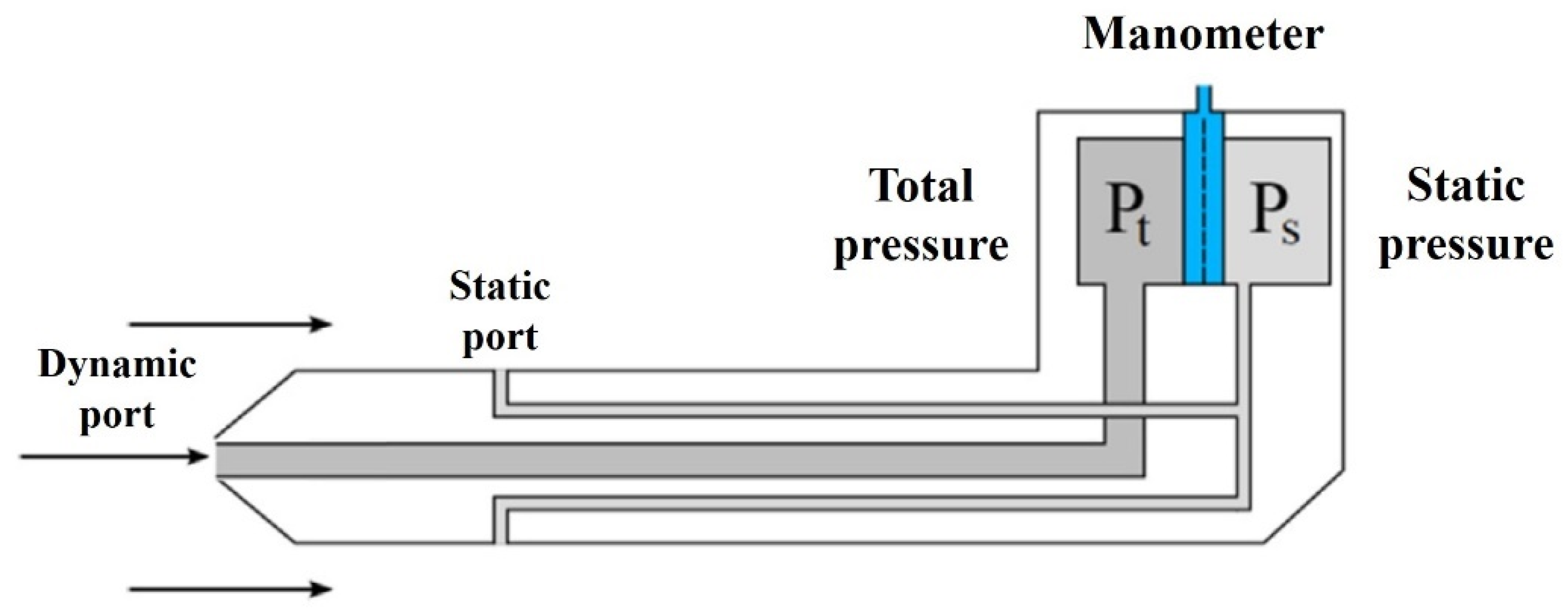
2.1.1. Pitot Tubes

The Pitot tube, also known as the Pitot probe, is used to determine the fluid flow velocity by directly measuring total pressure and static pressure from which the velocity pressure can be obtained. The device consists of a tube pointing directly into the fluid flow. When the fluid enters the tube (from the dynamic port, see Figure 1), where it is brought to rest, the stagnation pressure (or Pitot pressure) is measured. However, it cannot be used directly to calculate the flow velocity. Therefore, a manometer is connected to the tube allowing for the measurement of both the static (from the static port, see also Figure 1) and total pressures. The manometer will then display dynamic pressure, which can be converted into velocity. In modern Pitot tubes, proper nose or tip design, along with enough distance between the nose, static pressure taps, and stem, permit to minimize turbulence and interference.

Pitot tubes are easy to install, not expensive and, thanks to their size, they can be inserted into the fluid without interruptions. They also contain no moving parts, thus minimizing frictional losses. In addition, the pressure losses are very small and can be in-stalled even in extreme environments, in conditions of high temperatures and pressures. On the other hand, they can only be used in high-velocity flows, having low sensitivity and poor accuracy. Moreover, Pitot tubes do not permit to evaluate modifications in the velocity profile, as small velocity changes result in very low differential pressure, difficult to be evaluated. Finally, the measurements are affected by changes in the flow direction and are not suitable for dirty fluids or with sediments because they can easily become clogged with foreign materials in the liquid.

Recently, Pitot tubes have been used to evaluate the trajectory and speed of hybrid unmanned aerial vehicles with vertical take-off and landing (Ariante et al. [71]; Zhang et al. [72]). Fixed-wing unmanned aerial systems are also used for the study of turbulence in the atmospheric boundary layer and in the proximity of wind turbines. In the latter case, the aerial systems are equipped with multi-hole Pitot probes, calibrated through laboratory simulations to evaluate, with independent measurements, the uncertainty of statistical turbulence, flux calculations, and quantitative analysis of the turbine wake characteristics, varying the Reynolds number (Rautenberg et al. [73]). Furthermore, they allowed studying the gas-dynamic parameters of supersonic microjets, paying attention to Pitot pressure variations on the jet axis associated with the wave structure of the jet and to distortions of the supersonic core length (Mironov et al. [74]). In addition, Pitot tubes are used to measure flow velocity in narrow ducts (D’Amato et al. [75]) and in hydraulic jumps developed in stilling basins (Macián-Pérez et al. [76]).

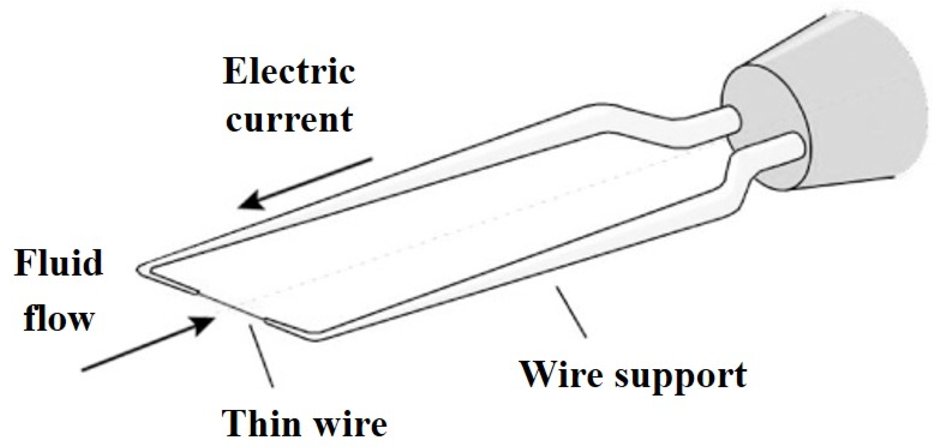
2.1.2. Hot Wire Anemometer (HWA)

The Hot Wire Anemometer (HWA) is a thermal transducer widely used to calculate instantaneous flow velocity from electric voltage measurements in airflows. The sensor consists of a very thin wire typically made of platinum or tungsten, usually hundreds of microns long and about 5 µm in diameter—which dictates its spatial resolution—connected to a measuring bridge (Figure 2). When the wire is fed by an electric current, it heats up until it reaches a temperature higher than that of the fluid in which it is immersed. The flow passing through the wire tends to cool it, and the cooling rate depends on the flow velocity.

HWA, although very delicate, has an extremely high-frequency response and allows measurements with high spatial resolution compared to other traditional techniques. Moreover, HWA is available as single-point instruments for test purposes, or in multi-point arrays for fixed installation. The main advantage of using HWA is that, by increasing the ratio between the length and the diameter of the probe, the temperature distribution around the wire is more homogeneous and the influence of the sensor on the flow is less. On the other hand, however, by increasing this ratio, the mechanical stability of the probe decreases. A single hot wire can measure the norm of the velocity vector if the plane in which the velocity vector lies is known (in most cases, the probe-stem is perpendicularly aligned with the mainstream direction of flow) but cannot give any directional information. In order to add directional sensitivity, two slanted wires (X-shaped probe with two crossed wire) may be used to obtain transverse velocity components: in this case a two-channel apparatus is needed for simultaneous measurement of two signals (Lomass, 1986 [77]). Obtaining accurate point measurements of mean and fluctuating velocities is difficult in reverse flow regions and standard hot-wire anemometry is virtually useless unless complex hardware and software systems are employed (Bruun 1995 [78]). To perform this kind of measurement, either Laser Doppler Anemometry or Pulsed Wire Anemometry (LDA and PWA, respectively, see below) are needed (Bradbury, 1976 [79], Heist and Castro, 1996 [80]), even if the HWA can be successfully used in the separated flows outside the reverse flow region (see, e.g., Leder, 1991 [81], Boiko et al., 1991 [82], Torii and Fuse, 1993 [83]).

Figure 2. Schematic of a hot wire anemometer (modified from Stornelli et al., 2017 [84]).

Figure 2. Schematic of a hot wire anemometer (modified from Stornelli et al., 2017 [84]).

HWA is used more frequently for scientific than industrial purposes. In fact, the fine wire probe is fragile and sensitive to contamination and, therefore, usually is not appropriate for industrial environments. Furthermore, the wire temperature is often too high for low-speed measurements, as strong natural convection from the wire can cause non-negligible errors. For this reason, these sensors can be used in wind tunnels with velocities ranging between 0.25 m/s and 60 m/s (Wilson [85]), but also allow the investigation of supersonic flows (see, e.g., Kovasznay, 1950 [86], Weiss et al., 2001 [87], Sakaue et al., 2020 [88]): in this last case, the prongs have to be designed for minimizing parasitic effects of shock waves (Gatski and Bonnet, 2009 [89]). Finally, the temperature compensation is employed to correct for fluctuations in ambient air temperature, which may not be available or may not cover the desired operating range.

HWA has been also used to evaluate the velocity perturbations and the combustion instability characteristics of turbulence stabilized combustors (Hwang and Ahn [90]), and to study the turbulence intensity under a large range of temperature variation (Lee and Lee [91]). Since the end of the 1950s (Hinze, 1959 [92]) HWA can be used in a constant temperature mode, in which the wire resistance and wire temperature are kept virtually constant (see, e.g., Freymuth, 1967 [93]), avoiding burnout damages to the hot-wire sensor, irrespective of the flow velocity, compared to the constant-current anemometer (see, e.g., Yatskikh et al., 2018 [94], Inasawa et al., 2020 [95]). In this configuration, HWA permits the measurement of very rapid velocity fluctuations (Ligęza [96]; Ligęza [97]). Moreover, to improve the sensitivity of the HWAs, macro-sized double-walled carbon nanotube strands are developed (Wang et al. [98]) and sensors similar to HWA but with a shorter response time and made in all-silica are under development (Njegovec et al. [99]). Further technological progresses have made it possible to develop HWA sensors with low noise, low power, and miniaturization characteristics that are used in the study of insect biomimetic robots to understand the characteristics of real insect movement (Nam et al. [100]).

2.1.3. Hot Film Anemometer (HFA)

The Hot-Film Anemometer (HFA) is a thermal transducer similar to the HWA. The main difference is the structure of the sensor: HWA consists of a cylindrical quartz or glass core (typically, 0.25 mm long with a diameter between 50 and 70 µm), covered with a platinum or nickel film (less than 0.1 µm thick), which, in turn, is electrically insulated through thin quartz or ceramic coating (less than 2 µm in thickness). Since the rod is longer than the film, not negligible effects of the prongs on the flow are detectable only when the flow is almost parallel to the sensor in the immediate surrounding area. Furthermore, mechanical strength and film thickness are independent. The working principle is similar to that of HWAs, being HFA able to operate in constant current or constant temperature conditions. The main advantage, compared to an HWA, lies in the greater mechanical strength of the film sensor for similar electrical and thermal properties, and the increased robustness permits use of the HFA also to measure the flow rate of liquids, such as water. An evolution of the classic HFAs are the split hot-film sensors (Hoshino and Ito [101]), in which the film on a cylindrical rod is divided into two parts. In this way, it is possible to distinguish between flow components even in a plane almost perpendicular to the sensor.

In recent years, HFA is typically used wind-tunnel experiments to study the flow regime into pipelines (Kadam [102]), to investigate at laboratory-scale building models with particular architectural characteristics are reproduced (Tavakol et al. [103]), or to study the characteristics of indoor/outdoor airflow and pollutant exchange in buildings (Cui et al. [104]). Furthermore, HFA is used to calibrate three-cup anemometers (Bai et al. [105]) and in aerodynamics to evaluate boundary layer transition on an oscillating airfoil (Ikami et al. [106]).

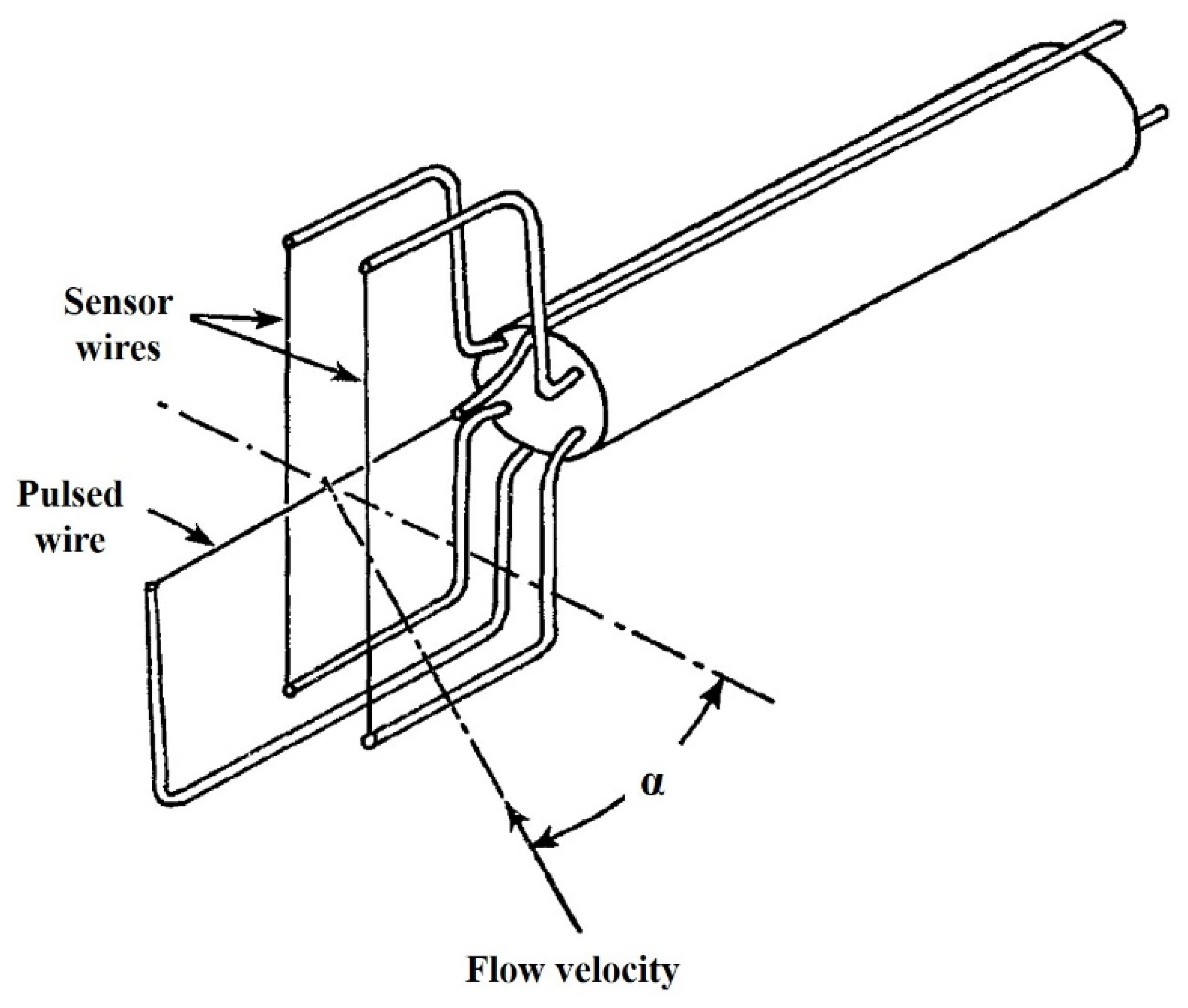
2.1.4. Pulsed Wire Anemometer (PWA)

Pulsed wire anemometer is a classical sensor introduced in the late 1960s and continuously improved. The velocity measurement is performed by timing the passage of a heat tracer between two thin wires (Figure 3). Again, as in the case of HWA and HFA, an electric current is generated and the sensor wires work as a simple resistance thermometer to detect the arrival of the tracer. Knowing the distance between the pulsed wires and the sensors, the instantaneous velocity of the fluid can be derived. So, in PWA, the output only depends on the velocity component in one predefined direction and it is capable of detecting when this component reverses flow direction: for this reason, it can be used successfully in the region of reverse flow of separated flows. Krogstad and Sinangil (1985 [107]) made comparative measurements between LDA (see below), PWA, and HWA in the near wake of a circular cylinder and concluded that the measurements using the PHWA are in good agreement with LDA data, even in the reverse flow region of separated flows, where the HWA limited directional sensitivity can lead to non-negligible errors (see also Kitzing and Sammler, 1984 [108], Handford and Bradshaw, 1989 [109], Bradbury, 1978 [110]).

The time interval required to cool the instrument determines the acquisition rate of samples. When flows with very low velocities are investigated, high sampling rates are required to have uncorrelated measurements.

One of the disadvantages of using PWA is the size of the probe, which is significantly larger than HWA and HFA. It makes this technique applicable only in relatively large-scale experiments. On the other hand, the instrument configuration reduces the noise of the instrument to the flow.

Historically, PWAs have been used to study flow behind slightly tapered cones (Bradbury and Castro [111]) and flows around obstacles (Hunt and Castro [112]).

As often happens with traditional techniques, PWA is nowadays often used as a support for other laboratory measurement techniques or to validate numerical simulations (Luo et al. [113]; Tominaga and Shirzadi [114]). For example, Brown et al. [115] used a wind tunnel with six canyons measuring flow velocity where the flow reaches the equilibrium. The same authors (Brown et al. [116]) performed a wind-tunnel experiment by measuring the velocity at different points and at different altitudes of a three-dimensional array of cubes.

2.2. Non-Intrusive and Quasi-Non-Intrusive or Minimally Intrusive Techniques

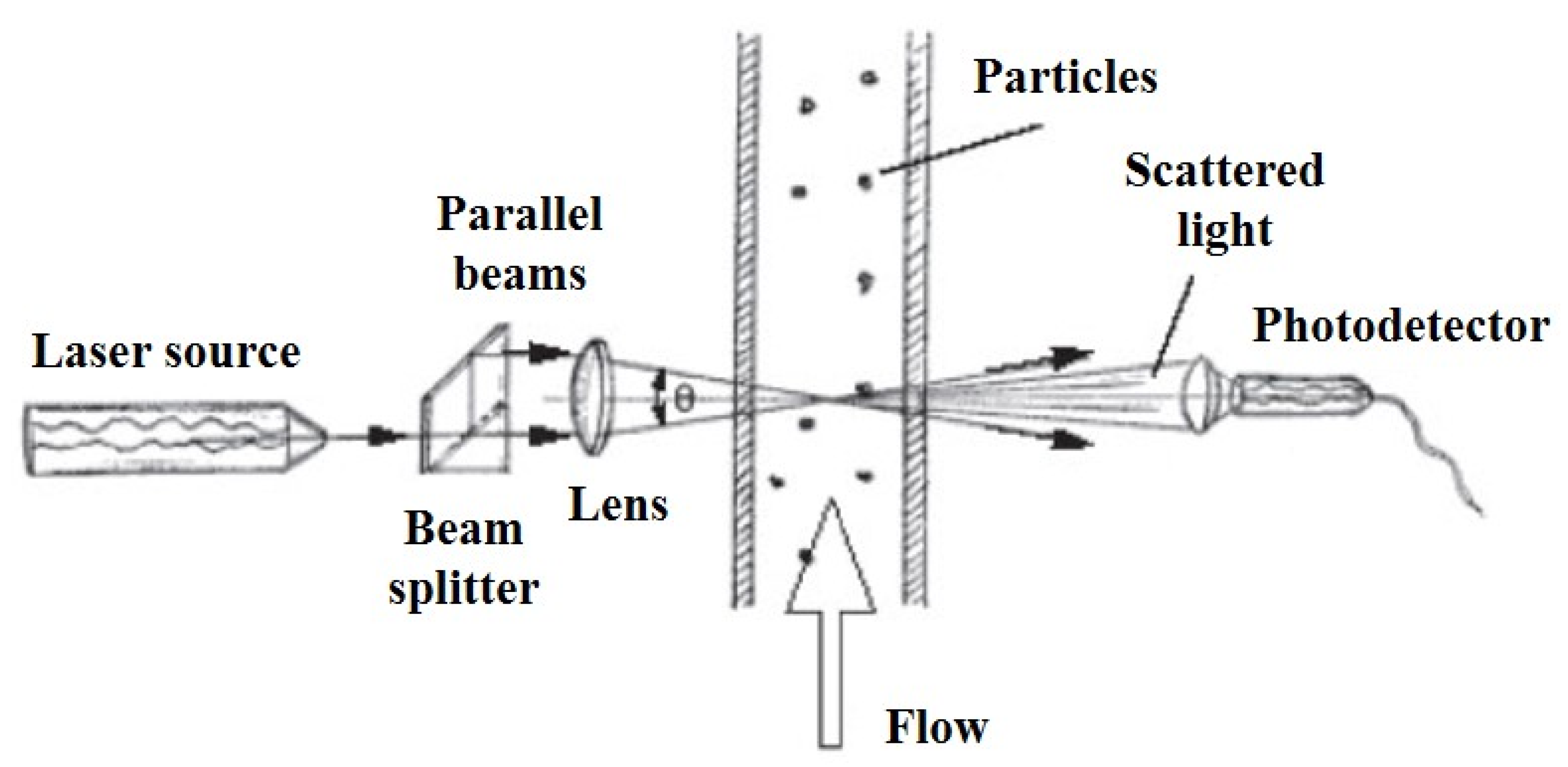
2.2.1. Laser Doppler Velocimetry (LDV)

Laser Doppler velocimetry (LDV), also known as laser Doppler anemometry (LDA), is a point-wise technique extensively applied to measure the local, instantaneous velocity in transparent and semi-transparent fluid flows and the linear or vibrational motion of opaque and reflecting surfaces. It is typically applied for the study of mixing, liquid flow, and energy dissipation in a variety of flow situations, including stirred bioreactors, nozzles, and combustion chambers. LDV was introduced in the 1960s and is based on the Doppler Effect. The light is emitted by a monochromatic, coherent, linearly polarized laser source and is split into two parallel beams with equal properties by a beam splitter (Figure 4). Both beams are refracted passing through a lens system and cross to form a fringe pattern. The local, instantaneous fluid velocity is computed by detecting the frequency of light scattered by small particles (typically 1–10 µm in diameter) suspended in the flow passing through a small control volume and assumed to faithfully following the flow velocity (Goldstein [117]). In fact, according to the Doppler principle, the frequency of the light scattered is shifted proportionally to the flow velocity. A photodetector is used to collect the scattered light and the particle velocity is obtained analyzing the wavelength (Durst et al. [118]; Tavoularis [119]).

High-spatial resolution measurements can be carried out traversing the sensor in the flow field. The dimension of the measurement volume determines the output spatial resolution. Classically, the measurement volume is 1–2 mm long and 100 µm wide. The temporal resolution is only limited by the intensity of the light scattered by the particles and by the number of particles suspended in the flow.

The main advantages of the LDV technique are: (i) the absence of disturbance to the flow to be studied, as this technique is non-invasive and does not require the positioning of probes within the flow itself, (ii) the high accuracy of velocity measurements without requiring a detailed calibration, (iii) the independence from temperature and fluid properties, and (iv) the possibility to measure any desired velocity component.

On the other hand, the main disadvantages are: (i) the need to inseminate the fluid if the number of particles already present is too low, (ii) the difficulty in making measurements crossing curved surfaces, and (iii) the impossibility of carrying out simultaneous measurements on several planar or volumetric points. To overcome these problems, generally, the walls of the vessels containing the fluid are made of transparent materials such as glass, acrylic plastic, and Perspex and, if the measurements fluid is water, silicon carbide, polystyrene, plastic, and metal-coated material particles with a diameter between 0.1 and 10 µm are generally added. Instead, to obtain information on multiple points, it is necessary to move the laser and the optics or the flow system so that the laser beams intersect at the different points of interest.

The sources of error of LDV measurements are mainly due to the inaccurate alignment of the laser source with respect to the point to be studied, to the finite time necessary for the particles to cross the control volume, and to variations in velocity within the volume itself.

After decades in which the LDV technique has been widely applied for single measurements, in recent years it has been generally coupled with other optical measurement techniques or has been used for the validation of numerical simulations. For example, Sayeed-Bin-Assad [121] used a 2D-LDV probe mounted on a 3D software-controlled traversing mechanism, flow visualizations, and Unsteady-RANS models to study the turbulent wake behind a semi-circular step cylinder with a constant flow rate. Their measurement volume was about 0.123 × 0.117 mm${}^2$ and water was seeded with polyamide particles. Agrawal et al. [122] used a water-channel facility and LDV to investigate intermittencies in low- and high-drag events in Newtonian fluid flows. They modified the transmitting optics of the LDV to measure the two-component velocity measurements very close to the wall by rotating the laser head by 45° about the spanwise axis to become closer to the bottom wall and by placing a biconcave lens in front of the laser head to increase the focal length of the laser beams. Moreover, Le Bideau et al. [123] used the LDV method to measure velocity profiles in order to validate the numerical output of a two-phase hydrodynamics model of alkaline water electrolysis for the production of hydrogen.

A similar technique to the LDV is the Phase Doppler Anemometry (PDA) (sometimes also known as particle dynamics analysis or with similar definitions). PDA relies on the same velocity measurement principle as LDV but in PDA the velocity value is measured by analyzing the frequency shift of light scattered by the flowing seeding particles in the measurement volume generated by of at least two intersecting laser beams. PDA allows the measurement of particle size as well (through the evaluation of the phase difference of the two incident laser beams, which is in fact proportional to the particle diameter), allowing the measurement of particle concentration and mass flux (see, e.g., Ofner [124]).

2.2.2. Digital Image Analysis (DIA) Techniques

Image-based measurement techniques in fluid flows have been employed since the 1970s, with the diffusion of high frequency cameras and digital images, which allowed to process, faster than before, groups of images of a flow. Suzuki and Shiozaki, in their paper from [125], employed high speed photography to analyze a combustion system for diesel engines. A second explosion happened in the 1990s and 2000s (Fernando [126]), when the increase in computation and storage capacities of computers allowed us to rapidly analyze the huge amount of data available from image-based technique experiments (Mayinger and Feldmann [127]).

In DIA techniques, one or more cameras (depending on the type of measurement carried on, planar, stereo or volumetric) shoot images of a lighted region of the investigated flow (a plane or a volume); in the case of planar measurements, the camera must be placed orthogonally to the illuminated plane (Figure 5). The cameras are usually equipped with CCD—Charge-Coupled Device or CMOS—(Complementary Metal-Oxide-Semiconductor) sensors, and can shoot images at a certain frequency and definition. The investigating region is usually lighted by one or more lasers (so the area of interest in the flow must have an optical access, e.g., a transparent wall), whose beams are modified into planes or volumes by suitable lenses. Laser emissions for DIA laboratory experiments can be continuous or pulsed; in this second case, the laser and the camera must be connected to a trigger, to ensure the image is shot while the investigation area is illuminated by the laser. The experiments are usually carried on in a non-illuminated dark laboratory and the flow is usually seeded with light-reflecting non-buoyant particles or dyes, depending on the target (velocity or concentration measurements) and on the applied technique, so a typical image displays some light regions (e.g., particles) on a dark background. On one hand, the DIA techniques have many advantages, such as: (i) the alteration of the flow is usually negligible; (ii) 2D and 3D spatial measurements can be rapidly achieved (many DIA techniques can even operate in real time); (iii) even if the directly measured quantity is the light intensity, many other quantities can be measured indirectly on the whole investigation field, e.g., the concentration or, when comparing the position of particles on two consecutive images, the velocity, vorticity and acceleration; (iv) the optical access needed for this techniques allow the investigator to look at the flow and see what is happening in the flow, which allows the researcher to draw first ideas on the flow properties (and, sometimes, adjust something that can be wrong in the experiment, e.g., unexpected level of turbulence) rather than wait for the data to be processed (and sometimes have to setup the experiments again). On the other side, the DIA techniques main disadvantages are: (i) frequency acquisition, i.e., in this case, the temporal distance between two consecutive images, is usually lower than the one achievable, at similar costs, with physical probes; (ii) an optical access to the area of interest of the flow is needed, which in some cases (e.g., industrial equipment) can be difficult, expensive or even impossible; (iii) a particular care must be given to the refraction index of the flow and of the optical properties of the optical access, which, e.g., in the case of curved surfaces such as in pipes, can alter the light and, consequently, the value of the measured quantities.

Particle image velocimetry (PIV) has become the most widespread techniques for velocity measurement in fluid flow (Westerweel et al. [129]). The term PIV first appeared in the scientific literature in the 1980s, in the paper by Pickering and Halliwell [130] even if this technique was already employed since the mid of the 1970s but under the name of Laser Speckle Velocimetry (Pusey [131]). In PIV, the flow is seeded with a high density of non-buoyant particles (much higher than the one allowed in particle tracking velocimetry—PTV, see below), and the velocimetry technique is based on digital image correlation—DIC, i.e., on the auto/cross correlation between a small interrogation window on an image taken at time t and the same window on the successive image, taken at a time t+$\Delta t$, but slightly shifted around its position on the first image: the distance between the first window and the window in the second image maximizing a given correlation function (i.e., the most similar to the first one) is considered the distance covered by the particles in the time $\Delta t$. This correlation, under the hypothesis of brightness constancy and small particle motion between the two images, is performed on a regular grid of windows and a single velocity is found for each window, usually containing a certain number of particles: so the measured velocity field is actually the mean velocity of that group of particles, reason why PIV is an Eulerian measurement technique. Relying on the comparison of two consecutive images, PIV is sometimes called two-pulse PIV, which means that usually PIV returns instantaneous velocity fields for each couple of images: if the temporal distance between couples of images is short enough to follow the flow structures, we can talk of time-resolved PIV, as firstly mentioned by Vogel and Lauterborn in 1988 [132]. On one hand, the high-seeding density allow the PIV to easily measure velocity field on the entire investigation field, and the adoption of correlation functions makes it a very robust method to digital noise, as stated, among the other, by Kahler et al. [133], who list the improvements of PIV techniques in terms of accuracy, resolution, dynamic range, and extension to higher dimensions. For instance, to improve the robustness of correlation, Falchi et al. [134] has developed and tested a robust image velocimetry (RIV), where, in place of the traditional auto/cross correlation, a more robust measure of the dissimilarity between interrogation windows is adopted. On the other hand, the spatial resolution is inversely proportional to the dimension of the interrogation window (the grid size). In addition to planar PIV, which allows to measure two components (2C) of the velocity field in a plane employing a single camera (2D-2C measurements), Stereo PIV (allowing 2D-3C measurements employing two cameras shooting the same illuminated plane from different angles and introduce by Hinrichs et al. [135]) and tomographic PIV (allowing volumetric 3D-3C employing at least three cameras and introduced by Brucker [136]) have been developed. Moreover, a four-exposure PIV system can be employed to measure the acceleration and pressure distribution in a flow field by comparing the velocity of the same group of particles at different times (see, e.g., Liu and Katz [137]). The widespread diffusion of PIV is proved by the large number of reviews available in the literature in different fields of application. For instance, Williamson et al. [138] and Noor and Johari [139] examined the employment of PIV to study laboratory models of hemodynamic flows with and without cardiovascular devices or artificial devices, highlighting that PIV have been mostly employed to investigate unstented models or intra-aneurysmal flow rather than peri or distal stent flow behaviors, and that PIV has been used both for standalone measurement and for validation of CFD studies. Jolley et al. [140] focused on the recent use of large-scale PIV and PTV for non-contact remote measurements in rivers, highlighting potentialities, and current drawbacks, e.g., the sensibility to the outdoor environmental conditions. Further, Scarano et al. [141] focused on large-scale PIV, but with attention to its use for industrial aerodynamics, introducing the fundamental principles of flow seeding with peculiar particles, the helium-filled soap bubble (HFSB), and showing data from experiments where the free-stream velocity of 50 m/s, which according to the authors can be considered the upper boundary with this type of measurements, is reached. Jena et al. [142] focused on the applications of PIV for the investigation of fluid flow and diagnostic purposes in internal combustion engine, highlighting how PIV can be an essential tool in this field, even if some challenges for its utilization for in-cylinder flow investigations still exist, e.g., the complication related to optical access in the intricate geometry of internal combustion engines or to the appropriate selection of seeding particles in a rapidly evolving ambient, involving fast combustion and chemical reactions. Blocken et al. [143] reviewed the employment of PIV (and LDA) and compared their capacity of providing accurate results, when compared to CFD, in the field reviews wind tunnel and CFD techniques to determine pedestrian-level wind (PLW) speed for outdoor comfort assessment. Cao et al. [144] have also stressed that the main reasons that allowed the PIV to become the most popular and promising technique for airflow field measurement in indoor environment in the last decade are the well-developed technologies, the great quantity of available experimental works and the large availability of commercially codes and ready for installation systems. Other relevant reviews about PIV can be found in the work of Adrian and Westerweel [145], Adrian [146], Buchhave [147], and Adrian [148].

Particle Tracking velocimetry (PTV) or low image density particle image velocimetry is an image analysis technique typically used to reconstruct the two- and three-dimensional velocity field of a fluid. The PTV allows reconstructing the trajectories of the particles, identifying the particles’ centers, and obtaining the components of the Lagrangian velocity of the moving particles, suspended in the fluid itself, by measuring their displacement in consecutive images recorded with a well-known frame rate. The acquisition system consists of four main components: illumination system, image recording devices, tracer particles, and algorithms for image evaluation. In order to use the PTV correctly, the density of the particles must be low enough to allow the identification of individual particles. From the direct measurement of the Lagrangian velocity, the Eulerian description of the flow can be subsequently obtained. Furthermore, the information acquired with the PTV permits obtaining information with high spatial resolution, guaranteeing the possibility of studying turbulent structures of small dimensions and with low-velocity gradients. On the other hand, the main disadvantages in the use of PTV reside in the high sensitivity to noise, the appearance/disappearance of particles within the single image due to transverse motions to the illuminated plane, and the superposition of the particles, which complicates their correct identification. Traditionally, this technique is widely used to study small-scale flows (Azadi and Nobes [149]) and to low-particle density flows (Cornic et al. [150]) but recently its use has also been expanded to large-scale indoor airflows (Fu et al. [151]) and to the investigation of the near-wall regions (Fu et al. [152]). Further recent studies used PTV to study the combustion of methane hydrate over a powder layer (Misyura et al. [153]), the activation of the low reactivity industrial fuel (Egorov et al. [154]), the effect of high-speed jets in highly abrasive environments (Riha et al. [155]), and velocity measurements in porous media (Sabbagh et al. [156]). In recent years, the evolution of PTV has mainly concerned technological and algorithmic development, leading to the definition of 3DPTV and 4DPTV. 3DPTV technique is able to detect the 3D particle position at high accuracy and at different successive time steps. It uses a multi-camera with a photogrammetric approach to measure the 3D velocity components, calculated from the relative displacements on each camera detector between two consecutive images that are subsequently translated into a 3D velocity field using a back projection. As a result, the 3DPTV allows to simultaneously capture time-resolved series of particle images to make an accurate reconstruction of the Lagrangian velocities by measuring on a statistically significant and independent number of samples in order to find a locally convergent solution by means of an appropriate media process. Moreover, it allows the estimation of other quantities fundamental for the in-depth study of turbulence—such as vorticity, shear, and normal stresses—and is used to study the role of coherent structures in the spatial/temporal development of momentum and energy exchange within the flow. Trieu et al. [157] used 3DPTV to examine the velocity of free surface flow using two photogrammetry-based PTV algorithms regarding different types of surface particles employed on the water flow. The increasing engineering interest in 3D measurements in fluid dynamics also manifests in the application of X-ray tomography (Weis and Schröter [158]), 3D PTV with digital holography (Wu et al. [159]), with the aim of also improving the reconstruction quality and improving the measurement accuracy and reliability (Bruecker et al. [160]). Otherwise, 4DPTV allows the reconstruction of the velocity field based on spatial (three dimensions) and temporal (plus one dimension) high resolution (Schanz et al. [161]). For example, this technique has been used to study the three-dimensional flow structure in stirred tanks (Kuschel et al. [162]). The inherent Lagrangian nature of PTV has allowed to develop techniques to measure the fluid particle acceleration, an intrinsically Lagrangian quantity (see Equation (1)), from the time derivative of velocity, which, in turns, is obtained as the temporal derivative of particles’ positions. Unfortunately, PTV techniques are very sensitive to measurement noise, which is amplified by the time derivative, so the acceleration measures can be very noisy. In La Porta et al. [163] and in the following works by Voth et al. [164] and Mordant et al. [165], a low-pass filter on the tracked particle positions was applied to reduce the measurement noise: this approach holds the main issue of the fixed size of the temporal window employed by the proposed filter, which is determined without particular physical consideration for each investigated case, with the target to not delete small flow fluctuations with a too large window size while still removing noise (which cannot be efficiently removed if the window size is too small). To overcome this issue with a physical-based criterion, Ferrari and Rossi [166] have developed a self-adaptive iterative method (Particle Tracking Velocimetry and Accelerometry, PTVA). PTVA relies on an adaptive number of tracked positions for the reconstruction of particle trajectories, depending only on the local flow properties, withdrawing some convection/sweeping information from the measures. PTVA has demonstrated to generate errors which are about six times smaller for the velocity and about four times smaller for the acceleration than the ones generated by methods employing a fixed window size. This technique has been then further developed by, among of others, Martinez et al. [167], in the framework of the development of a horizontal shock tube facility for measuring velocity and acceleration of shock-accelerated particles, and by Wang et al. [168], who developed an imaginary particle tracking accelerometry (IPTA) technique, where a polynomial fitting of the velocities along imaginary particle trajectories is applied iteratively, until reaching a convergence condition, in order to improve the accuracy of the acceleration measurement.

Particle streak velocimetry (PSV) can be considered as a subset of PTV, typically used to track objects moving at high speed in one or more directions. The PSV technique is based on capturing streak particles using cameras with a long exposure time. The streaks are essentially the tracks of the particles, the endpoints of each streak can be used to identify the position of a particle in the frame and, then, the curves that join them form a track of the particles’ displacement. Therefore, the instantaneous velocity field is obtained directly from the length of the streaks. PSV was a widely used technique before two-head pulsed lasers were available to researchers when the length of the streaks was manually assessed and converted into velocity vectors, through an onerous, time-consuming, and inaccurate process. Although in recent years this technique has been supplanted by PTV, it allows us to obtain more accurate and resolved values of the Lagrangian velocity, unlike the group Euler estimates obtainable from PIV and PTV. On the other hand, however, the PSV cannot be used in standard PIV configurations because the high spatial correlation of the particle streaks causes decorrelation and loss of precision in the results. In addition, the problems of overlap and occlusion, the high spatial uncertainty about the position of the particles, and the idea that the particle streaks are actually blurs and imperfections of the velocity field itself are among the most limiting factors. In recent years, PSV has been widely used in the study of turbulence in indoor environments (Voelker et al. [169], Fu et al. [151]). Moreover, significant technological advances allowed its application to 3D fields, leading to the definition of 3D-PSV (Zhao et al. [170]), and the color sequence particle streak velocimetry (CSPSV, Wang et al. [171]; Wang et al. [172]). Furthermore, the PSV technique has been improved by applying an ensemble of convolutional neural networks trained on streak images to draw a statistical prediction of the displacement magnitude (Grayver and Noir [173]), proposing evolutions of the traditional technique based on decaying streaks formed by individual phosphor particles following pulsed excitation (Fan et al. [174]), and improving the resolution of particle streak velocimetry (Tsukamoto and Funatani [175]).

Feature tracking (FT) is the name under which DIA techniques are classified for computer vision, which, when applied to measurements in fluid flow, are sometimes also called optical flows (OF). The flow is still seeded with non-buoyant particles and the experimental setup is the same as PIV and PTV, but the main difference with these is that the object to track is not chosen a priori (groups of particles in PIV and particles’ centers in PTV) but is defined as a feature that can be successfully tracked, which is a region in the image with high luminosity gradients in two directions. Feature tracking was firstly proposed by Lucas and Kanade [176] and further developed by Shi and Tomasi [177] in the field of computer vision, where the target was to track objects moving in space, where the features are most often corners or strongly textured areas in the image; in the area of optical flows, the best feature to track are usually borders of particles, where the largest brightness gradients are usually found. Features are then sorted according to their cornerness (i.e., the value of the 2D brightness gradient) and tracked between consecutive images in a similar way as the PIV correlation (usually minimization of the brightness differences, e.g., according to Miozzi et al. [178], employing the minimum of the sum of squared differences of interrogation window light intensities; the linearized equation governing the minimization problem is then solved only where the solution is guaranteed to exist). As FT tracks the single features, it returns Lagrangian measurements. Mendes et al. [179], have presented a comparison study of different OF methods (the most diffused ones by Lucas and Kanade, 1981 [176], Horn and Schunck [180], and Farnebäck [181], combined or not with the algorithm by Liu and Shen, 2008 [182]) algorithm), finding that the Lucas–Kanade method combined with the Liu–Shen algorithm provides the most accurate results for all the tested flow types and image conditions. FT has rapidly developed in a 3D velocimetry method, employed in various fields of fluid flows (e.g., in cardiovascular flows, Zhang et al. [183], in reactive flows for aerospace applications, Lauriola et al. [184], in high-speed train wake aerodynamics, Ferrari et al. [185], etc.).

The laser-induced fluorescence (LIF, acronym employed also for the light-induced fluorescence) takes advantage of the fluorescence property of certain substances, i.e., the property of a dye to emit light at a certain frequency when illuminated by a light (usually a laser coherent light at a fixed frequency). Since the first employment by Stewart and Judeikis [186], LIF has become one of the most widely used DIA technique to measure concentrations and temperature, in particular in gas application (Mayinger and Feldmann [127]). The working principle is simple, as the fluid under investigation is seeded with a fluorescent dye (e.g., Fluorescein or Rhodamine, see Melton and Lipp [187]), illuminated with a light at a certain frequency, then the concentration is linearly proportional to the intensity of the fluorescence signal, provided that the density of the dye is in the correct range, usually to be very low (Sutton et al. [188]). A calibration image of the lighted background must be acquired before the experiment, in order to measure the distribution of the light intensity in the investigated area and to ensure that the fluorescence intensity varies only because of the concentration. Moreover, a filter lens can be placed on the camera, in order to record only the frequencies emitted by the dye, even if this can decrease the amount of light recorded by the camera sensors. Further, the temperature can be measured by LIF, but with different techniques based, for instance, on the spectral analysis of the emitted light (see, e.g., the recent study of Orea et al. [189], about the most suitable tracer for high-temperature molten salt applications, of Zhu et al. [190], about the applications of LIF to the combustion diagnostics and practical engine measurements, or of McManamen et al. [191], about the shock-wave–turbulence interactions in high-speed flight and propulsion). LIF can be coupled with PIV to obtain simultaneous measures of concentration and velocity (see, e.g., Savitskii et al. [192], Zhang et al. [193], Charogiannis et al. [194]).

In the light attenuation (LA) or diffused back illumination (DBI) technique the area of interest must have optical accesses on both side, because on one side the camera is placed, while on the other side the light is placed: as the working fluid is seeded with a light absorbing dye (e.g., methylene blue), the light reaching the camera is absorbed by the fluid. As the light crosses the flow, the light has to be uniformly diffused in the investigation area (an image of the investigation area without flow should be taken before the experiments to calibrate the brightness in the recorded images of the flow) and the measured quantity is usually the integral of the concentration of the dye in the direction of the light. See Allgayer and Hunt [195] for a more detailed description of the principle of application of LA, in particular regarding the dye, the dye concentration, the illumination source and the more suitable optics. In Hacker et al. [196] a LA technique was used to investigate the mixing of fluid properties transported by gravity currents. Payri et al. [197], employed a DBI setup to investigate the behavior of liquid sprays injected through two singe-hole nozzles of different conicity, with the target to optimize the fuel consumption of direct injection diesel engines. In Choi et al. [198] the layer-averaged concentration fields of an inclined buoyant jet, discharged into a co-flowing current, has been studied by means of LA.

The temperature sensitive particles (TSPs) are employed to record temperature field: they can be prepared with different temperature sensitive dyes that have the capacity to change color depending on the flow temperature. In this way, a flow seeded with TSPs can be investigated via a DIA setup to obtain simultaneous measurement of temperature and velocity fields (as the particles’ displacements can be processed thorough PIV or PTV algorithm). The main problem is usually the calibration of the various used dye, because the quantity directly measured is a color intensity. In Someya et al. [199] the particles were luminophors, typically rare earth-doped ceramics. In Massing et al. [200], the particles were polymer particles doped with the temperature sensitive dye europium III thenoyltrifluoroacetonate -EuTTA- for the temperature measurement, and the nearly temperature insensitive dye perylene for the velocity one. Kim et al. [201] used thermographic phosphor tracer particles to simultaneously measure the temperature and velocity fields in a confined oil jet with high temperature. Zhou et al. 2019 [202] proposed an ex situ calibration of phosphorescence particles, usually calibrated in situ, to measure temperature and velocity fields in water droplets evaporating in an upward air stream. Burkle et al. [203] employed two different dyes, uranine and rhodamine B, to eliminate the influence of the droplet size in the temperature measurement, reaching very reduced uncertainties in the velocity (0.4%) and temperature (0.24 °C) with a high spatial resolution of 10 µm. An extensive review about TSP techniques and their coupling with velocimetry can be found in Someya [204], where a particular attention is given to the phosphor particles and to other dye-doped particles (more suitable for measurements in different flows and at different temperature), to their fabrication, limitations, and calibration.

2.2.3. Other Non-Intrusive and Quasi-Non-Intrusive or Minimally Intrusive Techniques

Schlieren (and shadowgraphy or other interferometric techniques, such as Moiré interferometry) takes advantage of the deflection that a collimated light beam experiences when crossing gradients of the index of reflection in a transparent medium, due to discontinuities in the fluid density. Even if it is a rather old technique, developed in the 1860s (Cheshire [205]), it is still often employed in particular to measure heat and mass transfer phenomena (e.g., Pellessier et al. [206] employed the Schlieren method for the investigation on pulsed synthetic jets for cooling applications) and to investigate supersonic flows (e.g., Yanhao et al. [207] investigated, via a high-speed schlieren system, the influence of the streamwise-pulsed spark discharge array to the incident shock wave/boundary layer interaction; Znamenskaya et al. [208] studied, via a schlieren technique and CFD simulations, the plasma formation impact on the supersonic flow over a blunt cone-cylinder).

Under the classification of light scattering (LS) fall various techniques relying on the light scattering phenomenon, i.e., the physical processes occurring when an incident light encounters a group of particles and is consequently partially absorbed, deviated or deflected. So, in a typical LS laboratory setup a light source before the investigation area and lenses and detectors after the investigation area are present. The role of the detectors is to analyze the scattered light to acquire information about the flow present in the investigation area. Depending on the specific scattering process, the LS can be classified as LDV (Mie scattering), Rayleigh thermometry, and spectroscopy (Rayleigh scattering), LIF (fluorescence), Raman spectroscopy (Raman scattering), etc. Without considering LDV and LIF, already faced above, Rayleigh thermometry allows the measurement of fluid temperature and density, Rayleigh spectroscopy of diffusivity and thermal conductivity, Raman spectroscopy of molecular concentration and temperature. LS techniques have been first developed between the end of 1800s and the beginning of 1900s and are still largely employed in investigations of fluid flows involving high velocity (i.e., supersonic flows, such as in Bowlan et al. [209], or in Kouchi [210]) or strong reactions (e.g., combustion, such as in Shariatmadar et al. [211], or in Franzelli et al. [212]).

2.3. Accuracy of Laboratory Techniques

In this section, as above stated, a brief discussion on the accuracy of the velocity measurement provided by the main techniques above described is provided, as this can help in choosing the proper technique depending on the specific scope of the measurement campaign. In fact, if on one-side imaging techniques can be very useful in providing instantaneous velocity fields (and are consequently more indicated for the first investigation of not completely known flows), the accuracy of velocity measurements with their help is frequently worse than with point-wise techniques, such as HWA (which are consequently more indicated for in deep analysis of already known flows). First of all, hot wire methods, thanks to their fast response and good spatial resolution, are irreplaceable for investigations of rapidly varying flows and, consequently, are the best method for measurement of velocity fluctuation in turbulent flows (see, e.g., Bruun, 1995 [78]). As a matter of fact, HWA is the only method for measurement fluctuations of order of several tens of kilohertz, as it has a very high frequency response (up to 500 kHz or even higher) and a high spatial resolution, as the measuring point is typically from 1 to 10 µmm in diameter and from 0.5 to 2 mm in length. The small measuring point is crucial, as high frequency fluctuations are connected with the smallest structures (vortices) in turbulent flows: for correct measurement of such structures the pressure transducers are disqualified because of too big measuring point. As for the accuracy, there are two factors. The first one is calibration and the second one is electrical noise. Every HWA probe should be calibrated and the precision of calibration determines the precision of the measurement (systematic error). For example, employing a calibration facility with standard precision, the error of the velocity determination is usually less than 1% (see, e.g., Jonáš et al., 2000 [213]) on the instantaneous and mean velocity evaluation. Electrical noise determines the random error of a given HWA: for instance, the high-precision laboratory device StreamLine by Dantec Dynamics Company (with high temporal resolution, as fluctuations up to 450 kHz can be measured, high spatial resolution, as eddies down to fractions of a mm can be resolved and high dynamic range, from a few cm/s to supersonic velocities, Dantec Dynamics, 2020 [214]) allows evaluation of intensity of velocity fluctuations about 0.1%. So, the typical error of the correctly applied HWA method is less than 1% on the mean velocity and about 0.1% on intensity of fluctuations (defined as a ratio of standard deviation and mean). Moreover, the turbulence spectrum of turbulent fluctuations can be evaluated easily, even if no calibration applied: the reason is that for spectrum mainly its shape (i.e., the −5/3 slope and possibly peaks–frequencies) is relevant, so in a log-log graph the noise could be determined as part of the spectrum with the slope smaller than −5/3, or even null, indicating white noise, which is typical for electrical noise but not in turbulence.

The LDA measurement does not require calibration and the experimental setup practically determines the measurement inaccuracy. In fact, the inaccuracy is primarily due to the alignment of the LDA measurement beams concerning the chosen coordinate system: the greater the deviation (angle) of these beams from the coordinate system, the greater the error. So, it is highest at an angle of 45° when the LDA does not know the correct direction and magnitude of the particle velocity. The inaccuracy is further increased by the boundary conditions of the measurement, such as whether the measurement is made through glass or other transparent objects. It is also important that the flow is sufficiently saturated by the passive sensors (the particles suspended in the flow) from which the beams are reflected by the LDA detector, as insufficiently continuous saturation causes incomplete time series and, in turns, the sampling rate that can be used to analyze the data; however, high sampling rates (up to 10 kHz) can be achieved with the LDA method, depending on the experimental setup, with an overall measurement error between 1 and 5% (see, e.g., Janke et al., 2020 [215]). The spatial resolution is related to the sizes of the measuring volume: Saga et al., 2000 [216], report about 65.3 µmm (volume diameter) × 0.68 mm (volume length). Uncertainties in velocity measurements from PIV depend on several different factors (see, among the others, Adrian and Westerweel, 2011 [145] and Raffel et al. 2018 [217]): on the acquisition frequency, on the sensor resolution, on the postprocessing code (e.g., the chosen window interrogation size and correlation scheme, and the peak-finding and sub-pixel peak fitting scheme), on the diameter and non-buoyancy properties of the seeding particles, on the particle image intensity distribution, on the background noise, on the displacement gradients within an interrogation window, on out-of-plane tracer particle motion, etc. If, on one side, pulsed-burst PIV can reach an acquisition frequency from 50 kHz (see, e.g., Price et al., 2021 [218]) to 1 MHz (Beresh et al., 2021 [219]), on the other side this can be reached with a lower image size and, consequently, a lower spatial resolution. A typical estimation of the error in PIV mean velocity measurement can be less than 3% (except where velocities are close to zero, Saga et al. 2000 [216]). Regarding the spatial resolution, as stated by Theunissen and Gjelstrup, 2018 [220], while PIV can provide velocity data within planar or even volumetric regions of the investigated flow, HWA and LDA can usually reach highest spatial resolutions: in particular, Lavoie et al. (2007) [221] quantified that, on their experiments, the HWA spatial resolution was roughly four times higher than that of PIV. The spatial resolution in PIV should be selected carefully if all the turbulent scales of interest (largest and smallest) are to be evaluated correctly: given a particular camera resolution, a compromise needs to be found between an image size large enough to capture the large scales and an interrogation window small enough to capture the small scales, while still providing an appropriate signal to noise ratio to minimize the number of spurious velocity vectors. Saga et al., 2000, [216] reached a spatial resolution of the order of 0.1 mm/px. Sciacchitano et al., 2015 [222], in the collaborative framework for PIV uncertainty quantification indicates a spatial measurement uncertainty ranging from 0.1 px to 0.05 px. Regarding the capability of PIV to properly measure power spectra, Beresh et al., 2021 [219], highlighted that, even if PIV multi-frame correlation analysis can reduce the error of vector computations summed over an entire data set, this does not imply that these improvements are observed at all frequencies, and their comparison with HWA data indicates that the high-frequency content of the spectrum is very sensitive to choice of the PIV interrogation algorithm and may not return an accurate response.

3. Numerical Simulations of Turbulent Flows

3.1. Turbulence Simulation and Energy Research

As noted in the aim of this journal, the general field of energy encompasses a very broad spectrum of applications, from technologies of energy supply, conversion, dispatch and final use to the physical and chemical processes behind such technologies. Still, despite such a wide range of phenomena and processes involved in energy research, the majority of flows occurring in such context are turbulent. Thereby, turbulence modeling and simulation techniques play a major and crucial role towards increasing the efficiency in energy harvesting, management, and consumption.

Since the first numerical solution of the Navier–Stokes equations presented in the work of Chorin in 1968 [223], the number of papers published in indexed scientific journals and conference proceedings with turbulence and simulation terms in title, abstract, or keywords, have seen an exponential growth with the advent of the computer era in the early 80s, with documents number doubling every year, and have reached a steady linear increase in the last twenty years, with almost 200 papers published annually (Figure 6). About 30% of papers have been published in the more general field of engineering and roughly 6% fall strictly in the field of energy. Among those, applications include sustainable energy, fuel processing, nuclear sciences, thermophysics and thermal sciences, combustion and fusion theory and modeling, propulsion, wind engineering, and building simulations, to cite a few, which clearly shows the large impact of turbulence modeling and simulation in the field of energy research (see also Table 3 in Section 4).

It must be noted that such a wide spectrum of applications involves an analogous wide spectrum of turbulent flows ranging from subsonic to supersonic regimes, fluids with complex rheology and flow with complex thermodynamic phenomena, such as multiphase flows with phase change and chemical reactions which would be impossible to discuss thoroughly in the present review. Therefore, even though the modeling techniques presented in the following (mainly DNS, LES, and RANS) are virtually applicable to any type of turbulent flow, the examples presented in this section will be limited to single-phase subsonic flows of Newtonian fluids.

3.2. Overview of Turbulence Simulation and Modeling

In a turbulent flow, a large spectrum of time and length scales intimately interacting with each other coexist. The separation between the largest and the smallest scales of turbulence increases with the Reynolds number $Re$. In the ideal case of homogeneous and isotropic turbulence, where turbulence characteristics are both independent of position and direction, and for sufficiently high Reynolds numbers, the Kolmogorov theory [225] predicts a separation between the largest and the smallest spatial and temporal scales of $R{e}^{3/4}$ and $R{e}^{1/2}$, respectively, thereby posing an enormous computational burden to the explicit simulation of turbulence, i.e., without the use of some level of empirical modeling. On the other hand, the interaction between turbulent scales, even when a significant separation occurs at high Reynolds numbers, and the different dynamic and characteristics of the large and small scales make it merely impossible to derive a universal model for the entire turbulent spectrum. Therefore, many simulation and modeling approaches have layered over the years and a significant research effort is still directed towards the development of new models and techniques to enable more accurate or more efficient predictions of turbulent flows.

Among all the numerical techniques and models available today, direct numerical simulations (DNS), large-eddy simulations, and Reynolds-averaged Navier–Stokes (RANS) simulations represent the three principal techniques and historic pillars on which the numerical simulation of turbulence was founded. An overview of the main characteristics of such techniques is provided here and a detailed discussion is presented in the following sections.

In a DNS, all essential turbulent scales are resolved directly and without introducing any level of modeling. Therefore, they are able to predict turbulent flows to a degree of accuracy comparable to laboratory experiments and, for this reason, DNS are also often referred as numerical experiments. On the other hand, the computational effort dictated by the separation between the large and small scales of turbulence is such to limit the applicability of DNS to flows at low Reynolds numbers and to simplified flow domains and, as such, to the realm of academic research. To the contrary, in RANS simulations the entire turbulent spectrum is modeled by estimating the effect of turbulent motions on the mean field via turbulence models, thereby reducing dramatically the computational effort required to run turbulent flow simulations even at high Reynolds numbers and in complex flow domains. However, the level of uncertainty introduced by turbulence models, which are mostly of empirical or semi-empirical nature, is such to require a careful preliminary evaluation when used within the context of a new application and only after a fine tuning of models coefficients is carried out very accurate predictions of turbulent flows are generally possible. A compromise between accuracy and computational effort is provided by LES, where filtering techniques are introduced to model only the computationally expansive small-scales of the turbulent spectrum via the so-called sub-grid models, while the largest scales are computed explicitly. LES belong to, and it is the main representative of, the so-called high-fidelity techniques for the simulation of turbulence, being capable of providing accurate results for a wide range of flows without the need of fine tuning the closure models as in RANS.

A visual comparison of DNS, LES and RANS simulations is portrayed in Figure 7, where the vorticity field computed by each technique for a turbulent flow over a backward facing step is presented at a given instant in time once a fully developed regime is reached in the simulations. The instantaneous flow structure provided by the DNS simulation resemble very closely that of a laboratory visualization, from which the broad range of spatial scales can be readily distinguished. In the LES map, a similar flow structure where the approaching flow separates from the step and becomes turbulent downstream can be observed, but the turbulent structures are now more blurred due to the filtering of the smallest scales performed, in this specific simulation, by the lower resolution of the computational grid. On the other hand, in the RANS simulation the instantaneous flow structure is completely lost due to filtering, both in time and space, of the entire turbulent spectrum. Therefore, only the mean vorticity map, representing the ensemble average of the instantaneous flow realizations provided by DNS and LES, is predicted by the turbulence model.

In Figure 8, the velocity history provided by the LES and RANS techniques at a given point in the turbulent separated region downstream of the step is presented in conceptual fashion starting from the original DNS signal showing, as expected, a high content of turbulent frequencies, from low modulation waves associated with the movement of large scale structures up to high-frequency oscillations due to disruption of large scales into smaller scales. The corresponding LES signal, obtained by spatially averaging the original DNS profile and shown by the continuous blue line in the plot, is able to provide an accurate representation of the low-frequency modulation whereas most of the high-frequency oscillations are lost. On the other hand, only the average value of the DNS signal, shown by the dashed black line in the plot, can be estimated within the RANS framework.

A picture of historic and current trends in the use of DNS, LES, and RANS techniques for the simulation of turbulent flows is presented in Figure 9, where the number of papers published in indexed scientific journals and conference proceedings with turbulence and names of different simulation techniques in title, abstract, or keywords are shown. From the end of the last century and up to the beginning of the era of turbulent flow simulations, the records are dominated by DNS and LES simulations, as most of the papers were dedicated to the understanding of the physics of turbulence and to establish the necessary knowledge to develop accurate and robust simulation tools for technical applications. Such trend has changed about half-way of the first decade of the new century, when RANS simulations have overtaken the number of published DNS studies and became as frequent as LES simulations. Further, while an exponential trend is observed at the beginning of the development and use of each technique, the number of published papers shows a linear trend in the last ten years, where RANS simulations seems to have surpassed the number of LES studies. Nonetheless, while the DNS trend shows a significant reduction in the number of papers published in the last decade, LES and RANS seem to have similar projections in the near future.

3.3. Direct Numerical Simulations (DNS)

The first direct numerical simulation of turbulence dates back to the pioneering work of Orszag and Patterson for homogeneous and isotropic turbulence [226], but it was only with the work of Kim et al. [227] that the more technically relevant problem of wall-bounded turbulence was approached for the very first time using DNS. A fully developed turbulent channel-like flow between flat plates was simulated at a friction Reynolds number $R{e}_{\tau }=u_{\tau }h/\nu$ of 180, where $u_{\tau }={({\tau }_w/\rho )}^{1/2}$ is the friction velocity and ${\tau }_w$ the wall shear-stress, corresponding to a bulk Reynolds number based on the bulk velocity and half channel height h of 3300. Turbulence statistics and statistical correlations were computed up to the wall and compared to existing experimental data finding an overall good agreement but also discrepancies that were mostly imputed to the accuracy of available measurements at the time, thereby already suggesting the complementary role of numerical simulations to laboratory experiments, which is very well established today. Flow visualizations using particle tracking were also reported and the structure and dynamic of near wall turbulence revealed for the very first time.

Since the work of Kim and coworkers, the boundaries of direct numerical simulations have been pushed thanks to the rise in the available computing power and through the development of more accurate and efficient numerical methods. About ten years later, Moser et al. [228] extended the work of Kim and coworkers using a friction Reynolds number $R{e}_{\tau }=590$, corresponding to a bulk Reynolds number of about 11,000, and reported quasi asymptotic behavior of turbulent statistics, suggesting universal behavior of wall-bounded turbulence at sufficiently high Reynolds numbers. Almost a ten times larger friction Reynolds number was achieved by Lee and Moser [229] almost fifteen years later, corresponding to a bulk Reynolds number of about 125,000. At such high Reynolds number regime, the existence of a logarithmic region in the mean velocity profile, whose characteristics have major implications for frictional losses in fluids and thus for energy consumption, is expected and was confirmed by simulation results.

DNS was also applied extensively to other types of canonical flows to investigate the similarity and asymptotic behavior of wall-bounded turbulence under simple-shear flow conditions. Spalart [230] performed the first DNS of a turbulent boundary layer over a flat plate subjected to a zero pressure gradient at $R{e}_{\theta }=U\theta /\nu$ of 1410, where $\theta$ is the momentum thickness of the boundary layer. A good agreement with available experimental data and theoretical results was found but the accuracy of the numerical solution was partly inhibited by the artificially applied streamwise periodicity used to handle the spatially developing nature of the boundary layer and limit the computational effort required by the simulations. Almost twenty years later, Wu and Moin [231] were able to perform a DNS of a zero pressure gradient turbulent boundary layer at slightly lower Reynolds numbers but without imposing artificial periodicity in the streamwise direction, thereby allowing the flow to encompass a natural transition from a laminar state at the inflow to fully turbulent conditions downstream. The intermittent localized disturbances arising from patches of isotropic turbulence introduced periodically from the free stream to promote the transition to turbulence proved to leave the dynamic of the transitional flow unaffected, which was then investigated in detail thanks to the accuracy and resolution of the DNS data. Several studies of fully developed turbulence in pipe flows have also been published starting from the work of Eggels et al. [232], where a friction Reynolds number $R{e}_{\tau }=180$ was simulated. The effect of the circular cross-section on the turbulent flow was analyzed by comparing turbulence statistics to the results of Kim et al. [227] for the plane channel, showing some discrepancies in the mean velocity profile near the channel center and a deviation from the logarithmic region predicted by theory. However, the most recent paper submitted on this topic by Pirozzoli et al. [233], where a DNS of the turbulent pipe flow is performed at a much higher, and the highest to date, friction Reynolds number of 6000, proves that the logarithmic region still holds in pipe flows and that a strong similarity between turbulent flows in pipe and channels exists. Moreover, visualizations of DNS results (see Figure 10 and also [234]) show that a strong similarity also exists in the structure and dynamics of near wall turbulence across the range of Reynolds numbers investigated in the paper ($R{e}_{\tau }=180÷6000$).

In the context of energy research, some examples can be also found in the literature where DNS has been used outside the domain of canonical simple-shear flows to address phenomena more readily connected to technical applications. In the work of Rie et al. [235], for example, DNS was used to investigate the near-wall thermal processes in an inclined impinging jet at low Reynolds number (Figure 11), a relevant topic for the design of highly efficient gas turbines operating at very high inlet temperature, where the design of cooling passages is crucial. Using DNS the authors were able to identify regions of counter-gradient transport, i.e., regions of the flow where heat is transported against the temperature gradient. This phenomenon may occur in complex turbulent flows and may undermine the prediction of heat transfer rates via RANS simulations when employing the standard gradient-diffusion hypothesis, where a perfect analogy between molecular and turbulent transport is introduced. Thanks to the extremely accurate and rich databases obtained by DNS simulations, improved models can be derived accounting for the counter-gradient transport mechanism (see also Rossi [236]). Since empirical modeling of the turbulent spectrum is avoided in a DNS, the main source of uncertainty in the numerical solution is associated with discretization errors arising from the numerical model adopted to approximate and solve the flow governing equations. Despite the fact that it is usually the entity of discretization errors, dictated by the order of accuracy of discretization schemes, which is of main concern in a numerical simulation, it is rather their nature that should be carefully evaluated when performing a DNS and, in general, high-fidelity simulations. The work of Felten and Lund [237] shows that energy-conserving schemes, regardless of their order of accuracy, are able to provide more accurate results when performing high-fidelity simulations of turbulent flows. Among other test cases, they performed an LES of a turbulent channel flow using a non-uniform grid in the direction between the parallel plates and compared a central scheme for convection discretization with mesh-independent weights, nominally first-order accurate but energy-conserving, to a second-order accurate and weighted scheme accounting for the grid stretching but unable to conserve-energy, showing better agreement in the mean velocity profile predicted from the low-order central scheme when compared to the reference DNS dataset. The work of Rossi [238] extended the analysis on the impact of discretization errors to DNS of scalar transport and found that high-order central schemes with correction for stretching and distortion, which guarantee second-order accuracy over irregular grids, may alter the turbulent spectrum in the range of the highest wavenumbers by adding spurious numerical modes. Since the scalar transport equation forms the basis for the simulation of heat as well as mass transfer in turbulent flow, the implications of numerical techniques employed to perform DNS simulations in energy research are thus evident. For an extensive review on the role of DNS in turbulence research, the reader is also referred to the work of Moin and Mahesh [239].

3.4. Large-Eddy Simulations (LES)

The idea of applying a spatial filter to fluid flow equations, which led to the birth of large-eddy simulations, was introduced in the late 60s within the field of meteorology by Smagorinsky [240] to solve a two-layer quasi-geostrophic model and represent large scale atmospheric motions. This filtering technique was then adopted by Deardorff [241] to perform, for the very first time, the simulation of the fully developed turbulent channel flow, but without solving explicitly the near-wall region. More than a decade later, Moin and Kim [242] performed the first LES of the turbulent channel flow by solving explicitly, albeit under-resolved, the near-wall region. Interestingly enough, both LES simulations of Dearforff and Moin and Kim preceded the DNS of Kim et al. [227], simply because at the time the available computational resources did not allow for solving all turbulent scales explicitly.

In LES the spatial filtering can be performed either explicitly by applying the filter to the numerical representation of the field variable function, such as in spectral methods, or implicitly. For example, in the framework of the finite-volume method, the grid size represents an implicit top-hat type filter leading to the filtered field variable (see Figure 12). Regardless of its formulation, once the spatial filter is applied to the flow governing equations, the filtered equations read as follows:

$$\begin{array}{c}\hfill \frac{\partial {\overline{u}}_i}{\partial x_i}=0\end{array}$$

(4)

$$\begin{array}{c}\hfill \frac{\partial {\overline{u}}_i}{\partial t}+\frac{\partial }{\partial x_j}\left({\overline{u}}_j{\overline{u}}_i\right)=-\frac{1}{\rho }\frac{\partial \overline{p}}{\partial x_i}+\nu \frac{{\partial }^2{\overline{u}}_i}{\partial x_j\partial x_j}-\frac{\partial }{\partial x_j}\left({\tau }_{ij}^{sgs}\right)\end{array}$$

(5)

where $\overline{(·)}$ denotes the spatial filter operator and ${\tau }_{ij}^{sgs}=\overline{u_i{u}_j}-{\overline{u}}_i{\overline{u}}_j$ the subgrid-stress or residual-stress tensor, consisting of all the contributions from the unresolved turbulent stresses and representing their effect on the resolved velocity field. In energy research, heat and mass transport or chemical reactions are frequently encountered; in these cases, a spatial filter can also be applied to a generic scalar transport equation which, after filtering, reads as follow:

$$\frac{\partial \overline{\varphi }}{\partial t}+\frac{\partial }{\partial x_j}\left({\overline{u}}_j\overline{\varphi }\right)=\nu \frac{{\partial }^2\overline{\varphi }}{\partial x_j\partial x_j}-\frac{\partial }{\partial x_j}\left(f_j^{sgs}\right)$$

(6)

where $f_j^{sgs}=\overline{u_j\varphi }-{\overline{u}}_j\overline{\varphi }$ is the vector of subgrid-fluxes, consisting of all the contributions from the unresolved turbulent scales and representing their effect on the transport of the resolved scalar field.

In order to predict the unfiltered velocity and scalar fields, a closure model is required for the unknown subgrid-stress tensor and subgrid-fluxes vector. Smagorinsky [240] proposed the first closure model for the filtered momentum equation via an eddy viscosity model, based on Boussinesq’s hypothesis [243], where the subgrid stresses are assumed proportional to the strain rate of the resolved velocity field:

$${\tau }_{ij}^{sgs}=2{\nu }_{sgs}{\overline{S}}_{ij}+\frac{1}{3}{T}_{kk}{\delta }_{ij},{\overline{S}}_{ij}=\frac{1}{2}\left(\frac{\partial {\overline{u}}_i}{\partial x_j}+\frac{\partial {\overline{u}}_j}{\partial x_i}\right)$$

(7)

In Smagorinsky’s model, a sort of mixing-length assumption is made, in which the eddy viscosity is assumed to be proportional to filter size $\Delta$ and to a characteristic turbulent velocity based on the second invariant of the resolved velocity field deformation tensor [244]:

$${\nu }_{sgs}={\left(C_s\Delta \right)}^2\left|\overline{S}\right|$$

(8)

where $C_s$ is the model constant. Along with eddy viscosity models, eddy diffusivity models are commonly employed for closure of the filtered scalar transport equation, where subgrid fluxes are assumed proportional to the gradient of the resolved scalar field:

$$f_j^{sgs}=-{\alpha }_{sgs}\frac{\partial \overline{\varphi }}{\partial x_j}$$

(9)

Although the modeling of ${\alpha }_{sgs}$ as a function of a set of selected basic quantities, similarly to eddy viscosity models, is possible, the eddy diffusivity is most frequently obtained by further assuming that the Reynolds analogy holds true for turbulent transport performed by subgrid eddies, thereby introducing a subgrid Schmidt number $S{c}_{sgs}={\nu }_{sgs}/{\alpha }_{sgs}$. The subgrid Schmidt number is usually assumed constant and therefore ${\alpha }_{sgs}$ is known once the ${\nu }_{sgs}$ is calculated [245].

The Smagorinsky’s model is very popular in engineering applications but suffers from several limitations, being excessively dissipative and not possessing correct asymptotic behavior in the near-wall region, thereby necessitating the use of ad hoc damping functions in order to be employed in the simulation of wall-bounded turbulent flows. Moreover, the model constant $C_s$ is strongly problem dependent and for specific applications model calibration might be needed for accurate predictions of the turbulent flow. In order to prevent the need for calibration, dynamic eddy viscosity models have been developed based on the idea of Germano et al. [246]. In a dynamic model, the model constant is locally calculated based on the information available from the resolved part of the velocity field, thereby allowing the model to be sensitive to the local structure of the flow and extending significantly its applicability. Nonetheless, the variability of the model constant can sometimes be severe and deteriorate the stability of the numerical method. For this reason, dynamic models are often coupled with averaging techniques of the model constant along existing homogeneous direction of the flow [247] or along the local trajectories of fluid particles for fully inhomogeneous flows [248]. Other types of models developed to improve over the performance of Smagorinsky’s model but without introducing the complexity of dynamic models exist, such as the model of Yoshizawa [249], where an additional transport equation is solved for the turbulent kinetic energy of subgrid scales, $k_{sgs}$, in order to compute the coefficient for the eddy viscosity, and the wall adapting local eddy viscosity (WALE) model of Nicoud and Ducros [250], where $k_{sgs}$ is estimated via a tensor based on the symmetric and anti-symmetric part of the resolved velocity gradient tensor, making the model sensible to rotation and providing the correct behavior in the near-wall region, thereby avoiding the need for damping functions. Other models and variants exist but a detailed analysis and description of subgrid-scale modeling lie beyond the scope of the present work. For a comprehensive review, the interested reader is referred to the work of Lesieur and Métais [244].

In LES simulations, the sub-grid modeling introduces some empiricism with respect to the full scale resolution typical of DNS. However, in LES calculations, the large amount of resolved scales (recommendation for LES simulations is to resolve no less than 80% of the turbulent spectrum [251]) and the richness of the associated turbulence dynamics are such that the importance of employing proper numerical techniques is still paramount. The guidelines concerning energy-conserving schemes presented in the previous section are thus still recommended. Nonetheless, the test cases presented in the work of Felten and Lund [237] deal with simple geometries and fairly regular grids, so one may wonder if the use of lower-order schemes with mesh independent weights may impair the accuracy of numerical solutions over grids of increasing complexity and thus lower quality. The answer can be found in the work of Mahesh et al. [252] where a low-order, co-located and energy-conserving numerical method has been presented and tested in complex geometries, including a gas turbine combustor with numerous passages, holes of various sizes and shapes, swirlers, and obstacles in the flow path. A comparison with experiments for the mass flow rate through the various components is made for the flow in the combustor, showing an average deviation below 5% for the LES simulation and thus validating the use of low-order energy-conserving schemes for complex, industrial-type, calculations.

The generation of realistic inflow conditions represents another issue and source of uncertainty, specifically for LES simulation. In fact, although DNS too requires the specification of boundary conditions at the inlet of the computational domain when dealing with flows that are inhomogeneous in the streamwise direction, they remain primarily a research tool and, as such, the necessity of generating inflow conditions able to mimic the variety of conditions found in technical applications, where a finite level of turbulence intensity is present in most cases, is far less stringent than in LES. Possible approaches for artificial generation of turbulent fluctuations at the inlet section of the computational domain are random fluctuations, precursor simulations, the recycling-method, and the synthetic-turbulence generation method [253]. In the random fluctuations method, uncorrelated spatial and temporal fluctuations are specified and, as such, they dissipate very quickly and do not satisfy the divergence-free constraint for incompressible flows, thereby introducing numerical instabilities. On the other hand, both the precursor simulations and the recycling methods are computationally expensive and generally restricted to simple flows in fully developed and stationary conditions. A significant research effort has been undertaken over the years towards the use of synthetic-turbulence approach, which was demonstrated to be the most promising method for the generation of realistic turbulent inflow conditions. Multiple techniques have been proposed based on the idea of Kraichnan [254], where sinusoidal modes are superimposed to the mean flow, and the digital filter method of Klein et al. [255], which is able to reproduce first and second-order one-point statistics as well as a locally given autocorrelation functions. These two techniques, however, present some drawbacks since only homogeneous statistics can be imposed using sinusoidal modes and a constant time-step and uniform grid are required by the digital filter. More recently, structure based methods have been developed and proposed, where turbulent structures are superimposed directly on the mean field allowing for inhomogeneous statistics to be adopted on non-uniform grids and variable time-steps [256,257].

Even with the current available computing power, the computational cost of fully resolved LES including the entire near-wall region, where most of small scale turbulent structures reside, still represent to date a limit to the applicability of LES simulations to high Reynolds number flows in complex, industrial geometries. Accurate estimates based on available knowledge of near-wall turbulent structures and consequent grid resolution requirements to capture such features show that the number of grid points scales with $\mathcal{O}\left(R{e}^{1.8}\right)$ when performing fully resolved LES [258,259], where $Re$ is the Reynolds number characterizing the flow. This means that even for a simple pipe flow at friction Reynolds number of ${10}^4$, corresponding to a bulk Reynolds number of the order of ${10}^5$, more than ${10}^7$ grid points are required to resolve explicitly the near-wall region [260]. Therefore, only massively separated flows will be affordable in the near future by fully resolved LES, since the large eddies have length scales that are dictated by the geometry and are not strongly dependent on $Re$ [261].

The computational cost of LES simulations can be greatly reduced by performing wall-modeled LES (WMLES), where wall-models are introduced to represent the inner, and computationally most demanding, part of the turbulent boundary layer [262]. Several models have been developed over the years mainly based either on the wall-stress-modeling approach or the hybrid LES/RANS method [263]. In the wall-stress-modeling technique (see the left side of Figure 13), the LES domain extends up to the wall but the grid resolution is such to resolve only the outer region of the boundary layer (located above $y^{+}>50$ for simple-shear flows, where $y^{+}=y{u}_{\tau }/\nu$ is the distance from the wall in viscous units, given by the ratio of friction velocity $u_{\tau }$ to the kinematic viscosity of the fluid $\nu$). The wall-stress model provides an estimate for the filtered wall shear stress, which serves as the boundary condition for the under-resolved LES grid where the no-slip condition cannot be applied directly [264]. In the hybrid approach (see the right side of Figure 13), the grid resolution is such to resolve the viscous region of the boundary layer (located below $y^{+}=5$), but the LES equations are solved only in the outer region while the RANS equations are solved in the viscous layer. There are advantages and disadvantages associated with both methods as well as several models and techniques developed over the year for estimating the filtered wall shear stress and handle the interface between the LES and RANS domains in the hybrid method, respectively. A detailed discussion of these topics lies beyond the scope of the present work and the interested reader is referred to the review of Piomelli and Balaras [262] for a comprehensive overview of WMLES.

Despite the apparent similarity with other numerical techniques for the numerical simulation of turbulence, such as detached-eddy simulations (DES) and the wall-functions approach in RANS simulations, it is important to stress that in WMLES only the inner part of the boundary layer is modeled whereas the energetic and dynamically important motions in the outer region are resolved explicitly. Therefore, WMLES has the potential to be significantly more accurate than DES. The computational cost of WMLES scales just linearly with $Re$ and therefore allows to broaden significantly the range of affordable flow regimes and applications for this method. In the recent work by Goc et al. [265], WMLES has been used along with the low-dissipative numerical schemes for complex geometries previously discussed and physics-based subgrid-scale models to perform, for the first time, accurate simulations of a realistic aircraft in landing configuration. Despite the additional level of uncertainty introduced by wall-modeling, simulation results are in very good agreement with wind tunnel measurement across a range of angles of attack, including maximum lift and post-stall regimes. The ability of WMLES modeling to resolve explicitly the outer part of the boundary layer also allowed for capturing and visualizing the complex near-wall flow structure (see Figure 14) and important features for the flow around the aircraft geometry in realistic flight conditions, such as the onset of inboard flow separation in the post-stall regime. The computing time of 7 h reported in the paper when running the simulations on GPUs (graphical processing units) for the largest grid employed in the analysis, about 160 M cells, suggests that WMLES may become a viable industrial tool in the near future for complex turbulent flows where not only the very large scales but also the near wall features must be properly modeled.

3.5. Reynolds-Averaged Navier–Stokes Simulations (RANS)

The first numerical computation of turbulent flows based on the Reynolds-averaged Navier–Stokes equations dates back to the early 1970s of the past century [266]. Thanks to the extremely low cost of RANS models, simulations of turbulent flows of practical relevance, such as wall-jets employed for cooling of turbine blades [267], have been performed using RANS more than a decade before the first ever DNS was attempted and more than three decades before LES of the same flow configuration at comparable Reynolds numbers was reported [268].

In the RANS framework, the entire turbulent spectrum is filtered in time to yield the Reynolds-averaged Navier–Stokes equations for the mean field, which read as follows:

$$\begin{array}{c}\hfill \frac{\partial U_i}{\partial x_i}=0\end{array}$$

(10)

$$\begin{array}{c}\hfill \frac{\partial }{\partial x_j}\left(U_j{U}_i\right)=-\frac{1}{\rho }\frac{\partial P}{\partial x_i}+\nu \frac{{\partial }^2{U}_i}{\partial x_j\partial x_j}-\frac{\partial }{\partial x_j}\left(R_{ij}\right)\end{array}$$

(11)

where P and $U_i$ are the mean pressure and mean velocity of the fluid, respectively, and $R_{ij}=\overline{u_i{u}_j}$ is the Reynolds stress tensor, consisting of the single-point correlations between the components of turbulent fluctuations $u_i$ and representing the effect of unresolved turbulent motions on the mean velocity field.

Similarly to LES, heat and mass transport simulations can be performed within the RANS framework by solving the temporally averaged transport equation for a generic scalar, which reads as follows:

$$\frac{\partial }{\partial x_j}\left(U_j\mathsf{\Phi }\right)=\nu \frac{{\partial }^2\mathsf{\Phi }}{\partial x_j\partial x_j}-\frac{\partial }{\partial x_j}\left(f_j\right)$$

(12)

where $\mathsf{\Phi }$ denotes the mean scalar field and $f_j=\overline{u_j\mathsf{\Phi }}$ the vector of turbulent scalar fluxes, consisting of the single-point correlations between the velocity fluctuations and the scalar fluctuations $\mathsf{\Phi }$ and representing the turbulent transport of the scalar field performed by the unresolved turbulent motions.

Similar to in LES, a closure model must be introduced to estimate the unknown Reynolds stress tensor $R_{ij}$ and turbulent scalar fluxes $f_j$ in order to predict the mean velocity and the mean scalar field using the RANS equations. The first closure model for the RANS momentum equations was proposed by Prandtl [269], starting from Boussinesq’s hypothesis [243] for the turbulent stresses:

$$R_{ij}=2{\nu }_t{S}_{ij}-\frac{2}{3}{\delta }_{ij}k,S_{ij}=\frac{1}{2}\left(\frac{\partial U_i}{\partial x_j}+\frac{\partial U_j}{\partial x_i}\right)$$

(13)

where ${\nu }_t$ is the eddy viscosity and $k=\overline{u_i{u}_i}/2$ the turbulent kinetic energy. In Prandtl’s model, the eddy viscosity is estimated as ${\nu }_t\sim u_t{l}_m$, where $u_t$ is a turbulent velocity scale and $l_m$ is the mixing-length. By introducing a perfect analogy with molecular transport processes, the mixing-length was used by Prandtl to compute the turbulent velocity scale as $u_t\sim l_m|\partial U/\partial n|$, where n denotes the shear-normal direction. Under these assumptions, the eddy viscosity becomes ${\nu }_t=C_m{l}_m^2|\partial U/\partial n|$, where $C_m$ is a model constant. Once a correlation for the mixing-length is provided, the model can be used to compute the Reynolds stress tensor and close the RANS momentum equations. Prandtl’s model represents an algebraic-type closure and, as such, comes at no additional computational cost. The model, however, can be only used for the simulation of simple-shear flows, such as flows in pipes and channels of very high-aspect ratio and one-dimensional, attached boundary layers, for which simple expressions of the mixing-length are available. Further, it is important to stress the perfect analogy between turbulent and molecular transport, where the mixing-length is taken as the equivalent of the mean free-path of molecules, does not hold outside the realm of simple-shear flows, where the mixing-length is generally not small compared to the scale of variation of the mean velocity, thus violating the hypothesis at the base of gradient-diffusion models valid for molecular diffusion processes [270]. Moreover, despite the similarity between eddy viscosity modeling adopted in RANS and LES closures, it is worth noting the gradient-diffusion hypothesis is employed in LES to represent only the small turbulent scales, showing stronger similarity with diffusion processes at molecular level [271]. Therefore, the modeling uncertainty associated with eddy viscosity RANS closures is, in general, far more significant than in LES.

Improved RANS-based predictions of complex turbulent flows can be achieved by abandoning algebraic modeling in favor of turbulence models based on differential transport equations used to compute explicitly the turbulent velocity and length scales employed in the definition of the eddy viscosity. These type of models are thus able to adapt the estimated eddy viscosity to local flow conditions, thereby improving significantly the predicted mean field using the RANS equations. Although one-equation models have been initially proposed, such as the Spalart–Almaras model specifically designed for aerospace applications [272], two-equations models, such as the $k-ϵ$ model by Launder and Spalding [266] and the $k-\omega$ model by Wilcox [273], are the eddy viscosity type closures most frequently adopted to predict turbulent flows in industrial applications. Both models are based on the solution of differential transport equations of the respective variables, i.e., the turbulent kinetic energy k, its dissipation rate $ϵ$ and the specific rate of dissipation $\omega$. In the $k-ϵ$ model, the eddy viscosity is estimated as ${\nu }_t=C_{\mu }{k}^2/ϵ$, where $C_{\mu }$ is a model constant, whereas the $k-\omega$ assumes ${\nu }_t=k/\omega$. It is worth noting the $k-\omega$ model was formulated in its original version to be used all the way to the wall and within the viscous sublayer, where the effect of viscosity is dominant and turbulent fluctuations are damped regardless how high the bulk Reynolds number of the flow is, without the use of damping functions. To the contrary, the standard $k-ϵ$ model is formulated for the fully turbulent flow regime and requires ad hoc formulations, usually termed low-Re, in order to be used to solve the inner part of the turbulent boundary layer (see e.g., the work by Jones and Launder [274]).

The $k-ϵ$ and the $k-\omega$ models, along with the Prandtl’s model, are also termed eddy viscosity models (EVMs) being based on Boussinesq’s hypothesis, where the eddy viscosity is used to compute the Reynolds stress tensor. Although eddy viscosity models with some variations have been employed successfully for virtually all practical engineering computations [275], the linear relationship between the Reynolds stress tensor and the mean strain rate adopted in Boussinesq’s model may lead to significant errors in flows where the anisotropy of turbulent stresses comes into play. For example, it is known that linear EVMs are unable to predict cyclonic flows [276], where the combined effect of swirl and streamlines curvature is such to determine a strong anisotropy between turbulence intensity in the axial, radial, and tangential directions [277]. Modified eddy viscosity models, where stress anisotropy is introduced via non-linear relationships between the Reynolds stress tensor and the mean strain rate, have been developed over the years to allow for improved predictions of flows dominated by rotation, curvature and other complex features (see e.g., Speziale et al. [278]). These complex flow features can be alternatively and more naturally predicted by the so-called second-moment closures, such as the Reynolds stress model (RSM) originally proposed by Launder et al. [279]. In the RSM, the transport equations for the six-independent components of the Reynolds stress tensor are solved, thereby implicitly embedding and providing predicting capabilities for complex flow features depending upon the anisotropy of Reynolds stresses. Such models, however, brings a significant computational overhead as well as reduced numerical stability due to the strong coupling between the transport equations of the individual stresses. For this reason, RSM type models have historically gained little popularity against EVMs (see Figure 15).

Compared to turbulent stresses, the modeling of turbulent scalar fluxes $f_j$ have received much less attention over the years. Nonetheless, the capability of solving the scalar transport equation may have a significant impact on energy research via heat and mass transfer simulations and therefore turbulent scalar flux models should also be carefully evaluated when dealing with complex flows. Similar to in LES, the modeling of turbulent scalar transport in the RANS framework typically relies on the standard gradient-diffusion hypothesis, where turbulent scalar fluxes are assumed proportional to the mean scalar gradient via the eddy diffusivity ${\alpha }_t$:

$$f_j=-{\alpha }_t\frac{\partial \mathsf{\Phi }}{\partial x_j}$$

(14)

where ${\alpha }_t$ is usually estimated via the turbulent Schmidt number $S{c}_t={\nu }_t/{\alpha }_t$. In the case of simple-shear flows, such as flows in pipes and attached boundary layers, $S{c}_t$ can be assumed reasonably constant (experimental measurements suggest a value of $S{c}_t=0.9$ in boundary layers while $S{c}_t=0.7$ for free-shear flows [275]) and the standard gradient-diffusion model provides reasonably accurate predictions of turbulent scalar transport. In complex turbulent flows, however, the isotropic nature of the standard model may lead to significant errors. The work of Rossi [280] shows that even in case of a two-dimensional, in the mean sense, velocity and scalar field behind an obstacle the standard gradient-diffusion hypothesis is unable to predict the streamwise component of the turbulent scalar flux. Although this may be of limited impact for a two-dimensional mean flow, a significant improvement in the accuracy of the predicted mean scalar field can be obtained when accounting for turbulent fluxes anisotropy in complex turbulent flows [281].

As a consequence of the high-level of uncertainty associated with the modeling of the entire turbulence spectrum and, for this reason, being a lower-fidelity method for the numerical simulation of turbulence, RANS simulations are less dramatically affected by the numerical methods employed for solving the temporally averaged momentum and scalar equations compared to DNS and LES. Nonetheless, since RANS modeling is more frequently employed to compute flows in industrial applications and therefore in complex geometries, the quality of the computational grid may have a significant impact on the accuracy of the numerical solution, especially in the near-wall region [282]. Particular care should thus be used, to the contrary of DNS and LES, in selecting numerical algorithms able to preserve their order of accuracy when employed over irregular grids [283].

3.6. Scale Resolving Simulations (SRS)

For almost four decades after the beginning of the era of turbulent flows computations, DNS, LES, and RANS have represented the only hierarchy of models for the numerical simulation of turbulence. Nowadays, a wider spectrum of models is available, ranging from partially averaged Navier–Stokes (PANS) to hybrid LES/RANS models as detached eddy simulations (DES) and more, where part of the turbulent spectrum is resolved explicitly, in the same spirit of LES, at least in one portion of the computational domain. For this reason, such models are termed scale-resolving simulations (SRS). It is worth noting a certain degree of arbitrary exists here in classifying one given model as belonging to SRS, as well as in considering one model capable of providing high-fidelity solutions of turbulent flows. For example, Unsteady-RANS (URANS) are able to resolve the largest scales the flow when sufficient scale-separation occurs, e.g., time variations that are of much lower frequency than turbulence as in vortex-shedding phenomena, but are unable to capture any portion of the turbulent spectrum even when the spatial and temporal resolution of the numerical model are increased [260]. On the other hand, the PANS method is not often included in SRS even though there is evidence of the capability of the model in reproducing part of the turbulent spectrum [284].

A visual comparison of scale-resolving simulations and standard RANS simulations is presented in Figure 16, where the turbulent flow around circular cylinder in cross-flow is simulated using the $k-\omega SST$ model of Menter [285] in steady and unsteady mode and the DES model proposed by Spalart [286]. In DES, the entire turbulent boundary layer on the cylinder surface, where the smallest and most computationally demanding turbulent scales are found, is modeled via the RANS Equations (10) and (11) whereas in the detached flow away from the cylinder surface, the LES Equations (4) and (5) are solved. As it can be noted, using the RANS model only the largest turbulent structures developing downstream of the cylinder are represented by the simulation, whereas a broadband spectrum is captured by the DES model. Moreover, as the grid is refined turbulent structures of smaller length-scale emerges from the simulation.

By modeling the entire turbulent boundary layer using RANS, the DES model is able to reduce significantly the computational effort compared to WMLES, where only the inner-layer is modeled, and dramatically compared to fully resolved LES (see Section 3.4). Nonetheless, the DES solution can depend critically by the reliability of RANS modeling of the entire boundary layer [261].

Several other SRS models exist but a detailed description and discussion lies beyond the scope of the present review and the interested reader is referred to the work of Spalart [286]. The practitioner may also find useful the best practices for scale-resolving turbulent flow simulations by Menter [260].

3.7. Numerical Methods and Codes for Turbulent Flows Simulations

Along with the development of new simulation techniques and turbulence models, the numerical methods and software used in turbulent flow simulations have also evolved over the years. As far as numerical methods are concerned, there are several properties characterizing each numerical technique which must be considered, such as accuracy, conservation properties, and spectral resolution, some of which have already been discussed in the previous sections. Since the impact of each property may vary with the level of turbulence modeling involved, if any, in the calculations, numerical techniques and numerical schemes must be carefully evaluated and selected depending on the type of simulations performed.

In the early days of turbulent flow simulations, when efficiency was of paramount importance due to the limited availability of computational resources, both DNS and LES simulations relied on spectral or pseudo-spectral methods, where high spectral resolution, i.e., the capability of a numerical method to represent the frequency content (either spatial or temporal) of a given function or signal, can be achieved with the highest possible numerical efficiency. Even today, despite pure spectral methods are limited to simple domains and simple boundary conditions [287], spectral codes are most frequently adopted when performing DNS simulations [288] because of the predominant use of this technique in turbulence research, where computational domains are typically of simple shape and one or more homogeneous directions exist in the flow.

On the other hand, with the ongoing effort towards evolving LES from a research tool to a design tool, there has been an increasing interest in unstructured finite-volume methods for high-fidelity simulations of turbulence [252]. In fact, despite the use of high-order finite-differences schemes with spectral-like resolution [289] and good conservation properties [290] has also been explored, the finite-volume method provides a framework where conservation can be more readily enforced while handling, at the same time, complex geometries more efficiently. Due to the limited connectivity between cells available in unstructured finite-volume grids; however, low-order numerical schemes are usually adopted in such context and despite the construction of high-order compact finite-volume schemes have been attempted in the past [291] in the spirit of the finite-difference method originally proposed by Lele [289], unstructured finite-volume schemes are usually limited to second-order accuracy.

A high-order accurate alternative for high-fidelity simulations of turbulence is offered by the spectral-hp method [292], which combines the geometric flexibility of the classical finite element technique with the desirable numerical properties of spectral methods, i.e., high spectral resolution, employing high-degree piecewise polynomial basis functions on coarse finite element-type meshes. However, the proliferation of this method has been limited by its complexity, which poses a challenge in the implementation of extended and multi-purpose modeling capabilities as well as in its use by practitioners.

The finite-volume method, originally in its staggered and structured formulation and nowadays in its co-located and unstructured derivation, used to be the preferred choice when performing RANS, i.e., low-fidelity, simulations of turbulent flows, due to their focus on practical applications. The numerical schemes adopted in such context are more concerned with their ability to preserve the order of accuracy over irregular meshes, albeit usually limited to second-order, which are customary in an industrial framework.

A comparison of the performance of some of the numerical methods mentioned above is possible for some benchmark cases available in the literature. Saini et al. [293] reported a comparison between the open-source codes OpenFOAM [294], based on the unstructured finite-volume method, and Nektar++, based on the spectral-hp method, for LES of a moderately complex geometry relevant to gas turbine combustor, showing better agreement with reference experimental data for Nektar++ for a given computational cost between codes or, viceversa, the same agreement could be obtained with OpenFOAM with 3.4 times more expensive simulation. Higher computational efficiency for the spectral-hp method was also demonstrated by [295] in the LES study of flow past a circular cylinder for Reynolds numbers ranging from 400 to 3900. The work of Goc [265] also provide a comparison between the computational cost between LES and RANS for the same benchmark case, a realistic aircraft in landing configuration, showing that it is possible to perform a medium-resolved LES for similar computational cost whereas a properly resolved LES required almost six times the computational effort of the RANS simulation.

It is also interesting to analyze the trend over the years in the use of in-house developed codes for turbulent flow simulations against commercially available and open-source software. In Figure 17, the number of paper published in indexed scientific journals with turbulence, simulation, and software types in title, abstract, or keywords is presented using Ansys Fluent [296] as the reference commercial code and OpenFOAM [294] as the reference open-source. From the plot it is clear that in-house software has already reached a plateau most likely due to its prominent use in academic research (further analysis of records based on the simulation type has not been attempted for the sake of brevity), whereas a constant increase in commercial software is observed. Nonetheless, OpenFOAM statistics highlight an a significantly increasing interest towards the use of open-source software for turbulent flow simulations and suggests a closing gap with commercial software in the future.

In the framework of high-fidelity simulations, i.e., DNS and LES, breakthroughs in available computational power and potential radical shifts in current computers’ architecture and programming paradigms will represent the most important advancements towards highly accurate simulations of turbulent flows in more complex, and complete, geometries of industrial relevance. The use of GPUs in place of CPUs, for example, has been explored and saw increasing interest from both the research community and industrial software vendors, with speed-ups of the order of 10x and more compared to CPU-based simulations, depending on the specific application as well as on the numerical method adopted in the computations [297]. The work by Goc et al. [265], where WMLES is applied to realistic aircraft in landing configuration (see Figure 14), shows about 25x speed-up in the turnaround time of the simulations when performed on GPUs thanks to the compressible and explicit nature of the solver used in the computations, fitting particularly well the GPUs architecture and operation [297]. Shu and Yang [298], reported a speed-up even higher, about 60x, for the simulation of turbulent mixing in a stirred tank using the Lattice Boltzmann method (LBM) and LES, thanks to the better suitability of LBM to GPU-based processing, while two order of magnitude of speed-up, about 150x, was obtained by Bieringer et al. [299] when using GPUs to form an ensemble of single-realization of pollution dispersion solutions using LES and coupled atmospheric transport (AT) and dispersion models. In order to fully exploit the potential of GPUs, however, significant investments in software development and technical collaborations between the research community and GPUs developers and vendors will be necessary due to the need for adapting the current established numerical methods to GPUs architectures [297].

Exascale computing systems, i.e., those capable of at least ${10}^{18}$ floating point operations per second (FLOPS) using CPUs, GPUs, or hybrid architectures, will also represent a leap forward in the achievable complexity and size of high-fidelity simulations of turbulence. It is interesting to note, however, that concluding remarks from the workshop Turbulent simulations at the Exascale: opportunities and challenges [300] stressed that even exascale computing will have an impact on the size and complexity of turbulence problems accessible, but only a modest increase in an achievable Reynolds number will be possible. Nonetheless, for some classes of problems even a modest increase may be transformative by exposing transition to new flow characteristics including, in the energy research context, the simulation of an entire wind farm under realistic atmospheric flow conditions and in complex terrain where turbine geometry is well resolved, thereby providing pathways to optimization and reduced cost of energy. To pursue such opportunities and to maintain the existing research capability on next-generation computer hardware, however, it will be essential for the scientists developing the algorithms and computational tools to adapt to the changes in the computer hardware. Without algorithmic and implementation changes, today’s petascale class turbulence simulations may take even longer to run on anticipated exascale hardware. Research work to move even beyond the existing classical computer architectures for turbulence simulations have also been initiated as in the work of Griffin et al. [301], where the use of quantum algorithms for direct numerical simulations has been explored.

As the complexity and size of high-fidelity simulations will increase, the need for cost-effective and highly efficient post-processing tools able to handle the enormous amount of data produced by DNS and LES will also increase. Research fields such as Artificial intelligence, data mining and machine learning can thus be foreseen to be playing an increasingly important role in this respect. In the case of direct numerical simulations, which will represent a research tool for many years to come and, as such, being focused on improving our understanding of turbulence dynamics, tasks such as features recognition will be subjected to automation and support from specialized algorithms in order to efficiently extract coherent structures responsible and associated with technically relevant phenomena. For example, it is well established that friction drag in wall-bounded turbulent flows is intimately connected to the momentum exchange between the near-wall region and the outer part of the turbulent boundary layer via the so called sweeps and ejections events. During the sweep event, patches of accelerating flow ($u>0$) move from the bulk region of the flow towards the wall ($v<0$), whereas during an ejection event patches of decelerating flow ($u<0$) move from the near-wall region towards the outer layer ($v>0$). Such mechanisms are, in turn, associated with the formation and subsequent breakdown of coherent structures in the form of hairpin-like vortices and lead to very high correlations in the components of velocity fluctuations and therefore to high Reynolds stresses [302]. In the work by Aguilar-Fuertes et al. [303], two machine learning techniques, the multi-layer perceptron and the long short-term memory, have been used and tested to automatically track hairpins vortices emerging in a turbulent channel flow. The algorithms were used in particular to predict at run-time the evolution of coherent turbulent structures by predicting geometrical features, such as the center of mass, the bounding box and the volume, at the time step $n+1$ by using and training the algorithms with the information available at the current time step n.

In the upcoming era of exascale computing, the need for post-processing of high-fidelity simulations at run-time will not only be dictated by process automation but also by the predicted impact of increasingly higher I/O streams from the simulation workflow, calling for the use of in situ post-processing techniques. An example of such techniques is given by quantitative imaging, i.e., images enriched with custom metadata that maps every pixel to its location in simulation space and any associated data value, sequences of which can be used, for example, to rapidly compute turbulence statistics at run-time without the use of any I/O call (Cascade [304], personal communication by Dr. Michael Emory).

While the increase in available computational power will affect less directly and dramatically the complexity and size of low-fidelity simulations of turbulence, where turbulent scales are not resolved explicitly and therefore the computational cost greatly reduced, artificial intelligence will have a significant impact in improving the modeling accuracy and predictive ability of RANS models in the future. Using machine learning techniques, for example, it is possible to potentially establish the relation between closure models coefficients and the mean flow field using data from high-fidelity simulations or measurements data [305] instead of relying on manual fitting of simulations results against reference datasets. Duraisamy and Durbin [306] applied artificial intelligence to model bypass transition using intermittency transport models and experimental data, inverse solutions were used to extract modeling information from reference data and machine learning to convert information into modeling knowledge, resulting in successful reproduction of the measured data used for training.

Another important and already established future direction in the field of RANS simulations is the so-called uncertainty quantification (UQ) [305], where the variability of input parameters to the simulations, such as the inflow conditions, and the effect of modeling parameters, such as the coefficients of turbulence models, are evaluated in order to interpret simulations results in probabilistic terms and provide a confidence interval to the low-fidelity numerical predictions. Both artificial intelligence and advances in computational resources will have an impact on uncertainty-quantification methods. Machine learning, in fact, can be used to better identify and quantify uncertainty associated with turbulence models [307], whereas the larger computational capacity which will be provided by next generation computing platforms will allow for perform more easily multiple simulations with perturbed parameters or initial/boundary conditions needed to for UQ as well as for design exploration [300].

4. Discussion: Advantages and Disadvantages, Challenges, Trends, and Taxonomic Analysis of Laboratory and Numerical Techniques

As discussed in details in the respective sections, both laboratory and numerical techniques have nowadays reached a mature status and are able to provide affordable data in various fields of engineering where turbulent flows play a dominant role. Nonetheless, the two techniques still have some peculiarities that can make one or the other a better choice for specific problems to be investigated. For example, while at the early stages of the numerical simulation of turbulent flows the costs, both in terms of computing time and hardware, were relevant, today both the software and hardware required to run turbulent flow simulations for industrial geometries at realistic operating conditions, at least within the RANS framework, have become accessible even for medium and small industries at affordable costs. Moreover, some specific codes are open source and commercial software have reached a level of automation such as to not require specific skills and expertise anymore. However, this also opens a potential conflict between accuracy and robustness of numerical results and the “democratization” of numerical simulations pursued by many legacy software developers and distributors. On the other hand, laboratory simulations still bear higher costs to be performed, because of the instrumentation and dedicated environments needed, but are usually performed by specialized technicians and scientists and, therefore, there are less possibilities to acquire nonphysical results. This is even more true for new and unexplored fields of application of numerical simulations of turbulent flows.

An emblematic case is represented by the simulation of thermally driven turbulence or turbulent Rayleigh–Bénard convection, which governs turbulent flows in the atmosphere for meteorological forecasting and climatological studies (Hartmann et al. 2001 [308]), in oceanography for the analysis of thermohaline circulation driving deep-ocean circulation (Marshall and Schott, 1999 [309]), and for studies on melting ponds (Scagliarini et al. 2020 [310]). Due to the high complexity of these phenomena, generally the turbulent Rayleigh–Bénard convection is studied with the Eulerian approach, focusing on local and global turbulent heat transfer processes (Grossman and Lohse, 2000 [311]; Chavanne et al., 2001 [312]; Lohse and Xia, 2010 [313]), while Lagrangian analyses are still rare (Schumacher, 2009 [314]). The most recent technological developments have made it possible to develop laboratory simulations for the study of the velocity field by creating a large convection cell (Xia et al., 2003 [315]), for the analysis of biphasic flows (Wang et al., 2020 [316]) and for the investigation of the interaction between urban heat island and sea-breeze regime (Cenedese and Monti, 2003 [317]). However, the investigation with laboratory simulations of the thermally driven turbulence is still quite rare due to the difficulties related to the creation of a stable setup and this problem is far from full understanding, yet. Typically, numerical simulations are preferred to study the role of buoyancy in the breakup criteria of drops or bubbles (Liu et al., 2021 [318]) or to examine the dynamics and structure of large-scale circulation under inhomogeneous boundary conditions (Vasiliev and Sukhanovskii, 2021 [319]).

Another challenge to be faced for the complete understanding of turbulence is the comprehension of stratified flows, particularly interesting for the analysis of the atmospheric nocturnal stable boundary layer, in which the turbulence has local origin and the structure of the surface layer obeys the Monin–Obukhov similarity theory (Obukhov, 1946 [320], Monin, 1954 [321]), and the mutual interaction between sub mesoscale motions and turbulence (Staquet and Sommeria, 2002 [322]). The formation of sub mesoscale waves in katabatic flows caused by the rupture of turbulent jets has been demonstrated through laboratory (Dohan and Sutherland, 2003 [323]) and numerical (Renfrew, 2004 [324]; Largeron et al., 2013 [325]) simulations. Furthermore, the scientific debate concerning turbulence in rotating flows appearing in several geophysical and industrial applications, in which extremely complex spatial structures develop (Godeferd and Moisy, 2015 [326]) is still open.

The realistic simulation of turbulence is challenging also for the study of biological systems, mainly related to the human body, with the aim of improving the quality of life and optimizing the prototypes developed in the field of biomedical engineering. In this field, recent numerical simulations, guided by ever more accurate three-dimensional models of organs and tissues, have made it possible to simulate the turbulent airflow in human respiratory tract (Srivastav et al. [327]), the coronary arteries under stenotic condition (Mahalingam et al. [328]), and the aerosol deposition in the nasal cavity (Liu et al. [329]), among others. The realization of setups for the experimental study of turbulent flows in biological systems is certainly complex, although not impossible. As instance, Fortini et al. [330] used image analysis techniques to reconstruct the mean velocity and turbulence field in a human ventricle model, Gülan et al. [331] used 3D-PTV to examine turbulent flow in the ascending aorta, while Boutsianis et al. [332] used PTV to investigate the turbulent flow characteristics during abdominal aortic aneurysms. Modern metrology used in experiments permit to obtain a refined picture of the velocity field topology and of the axisymmetric velocity field statistics, including high-order moments, by applying image analysis techniques such as PIV and PTV (Praud et al., 2006 [333]; Van Bokhoven et al., 2009 [334]; Moisy et al., 2011 [335]). Nonetheless, experimental scientific progress is still limited in this sector as the evolution of turbulent structures is due to the simultaneous effect of edge effects, shear, rotation, and stratification (Davidson, 2013 [336]). From the numerical point of view, introducing the Coriolis force can be much easier than in experiments (Teitelbaum and Mininni, 2010 [337]) and the larger resolution direct numerical simulations guarantee the correct separation of the turbulence scales. Nevertheless, many challenges remain open, such as the coupling of rotation and stable stratification effects (Godeferd and Moisy, 2015 [326]).

In the context of numerical techniques, turbulence modeling remains crucial in order to improve the accuracy and capabilities of turbulent flow simulations. One of the latest attempts stems from fractal geometric considerations, which lead to new turbulence models that are not only nonlinear, but also nonlocal and fractional, whereby these two features have most properties in common. To cope with Kolmogorov’s inertial range spectrum of turbulent eddies and its extensions including intermittency, Chen has started with a nonlocal description by introducing into the Reynolds shear stress a fractional derivative (Chen [338] and Chen et al. [339]). Several other authors have taken up this recipe and have generalized their corresponding Reynolds stress modeling (Churbanov and Vabishchevich [340] and Di Leoni et al. [341]). Different authors have preferences for different fractional derivatives, e.g., Sousa introduces in his model of turbulent diffusion the Riesz fractional derivative (Sousa [342]). Research on fractional partial differential equation modeling (FPDE) for turbulent flow fields near solid walls have been reported by Keith et al. [343]. Egolf and Hutter [344] report on the difference-quotient turbulence model (DQTM), which is a generalization of Prandtl’s mixing length and shear layer model and copes directly with fractional properties in correspondence with Lévy flights, related to clustering spatial eddy distributions. Such models and their developments are ready to in the near future replace simple gradient-based turbulence models with their insufficiencies. However, not every case has the transformation to simple applicable numerical algorithms been outlined yet. The first promising attempts have been undertaken by Samiee et al. [345] and Seyedi and Zayernouri [346] and applied to LES turbulence modeling.

In order to support what was stated above, but also to highlight the trends in the research on turbulence, a bibliometric analysis has been performed through the research and analysis tools of the scientific database Scopus [224]. The relevance of the turbulence field in the scientific community can be estimated comparing the total number of indexed documents in Scopus (around 80 million) to the total number of documents containing the word “turbulence” in the title, abstract or keywords (226,787 on 7th February 2022): the research on turbulence turns out to be around 3‰ of the total produced research. In

Table 1. Percentage of the subject areas of the papers published in indexed scientific journals and conference proceedings with the word “turbulence” in title, abstract, or keywords (source: Scopus.com).

Subject Area	%
Engineering	28.99
Physics and Astronomy	20.85
Earth and Planetary Sciences	9.50
Chemical Engineering	7.38
Mathematics	5.65
Energy	4.98
Materials Science	4.85
Environmental Science	4.44
Computer Science	4.42
Chemistry	2.59
Agricultural and Biological Sciences	1.50
Other	4.84

, the distribution of subject areas of those documents is reported: under “Other” are grouped areas weighing less than 1.00% on the total. Most of half of all the research on this field is in the area of engineering and of physics and astronomy, with the energy field which concerns almost 5% of the total. The prevalence of engineering (together with other areas of applications such as energy, material science, environmental science, etc.) highlights the practical relevance of the research on turbulence, whilst the weight on the total of areas such as physics and astronomy or mathematics recalls the unsolved questions that turbulence still carries on.

The tendency of the research on turbulence can be estimated from Figure 18, where the papers indexed in Scopus until 2021 (entries from 2022 have been neglected because the data are too partial, as the database was accessed the last time on 7th February 2022) have been plotted versus the year of publication. The data set consists of 225,115 documents, starting from the first one of 1915 by Humphrey and Hatschek [347], regarding an laboratory experiment about the viscosity of suspensions of rigid particles at different shear rates. After about fifty years of a very slight growth, almost invisible from the figure due to the scale, from the mid of the 1960s this growth has been very fast, with a further increase at the beginning of this century, highlighting the growing interest about this field.

Given the topic of the present review paper, the trends of the employment of laboratory or numerical techniques have been analyzed. In order to do this, the data-set of documents containing “turbulence AND experiment OR laboratory AND NOT numerical” has been examined to estimate the laboratory investigation on turbulent flows. This data-set consists of 26,755 papers, starting from the first two from 1920 of Mackenzie and Honaman [67] and of Tice [68], related to the optimization of fuel consumption and of cylinder combustion in engines. Regarding the numerical investigations on turbulent flows, these have been estimated from the data-set of documents containing “turbulence AND numerical AND simulation AND NOT laboratory”. This data-set is made up of 44,689 papers, starting from the first two dating back to 1969 (Lilly [348] and Orszag [349]), where some schemes for the numerical solution of the Navier–Stokes equations (at moderate Reynolds number in two-dimensional incompressible approximation) are presented. It should be highlighted that this bibliographic analysis is intended to give an estimation of the trends and not the exact distribution of the two approaches, as can be seen, for instance, by the fact that the sum of the laboratory data-set with the numerical one does not correspond to the total number of documents containing turbulence: this can be due, for example, to fact that not always authors write the search terms here employed in the title, the abstract, or the keywords (as in the above quoted work of Humphrey and Hatschek [347] from 1915, which is a laboratory investigation but where the search words here employed are not included), preferring to directly indicate the technique adopted. Moreover, some papers are about theoretical models or field measurements, etc. The two data-sets are plotted in Figure 19 versus the year of publication: laboratory data are in blue, numerical ones in red. The figure shows that, from 1969 till 1994, the laboratory techniques were prevailing, from 1995 till 2001 numerical techniques were just a bit more employed than laboratory ones (but with similar values), while from 2002 till present the distance has gradually increased, with studies employing numerical techniques, which nowadays, are much more than twice (almost three times) the laboratory ones.

In

Table 2. Subject areas of laboratory research in turbulence: percentage of the subject areas of the papers published in indexed scientific journals and conference proceedings with the words “turbulence” AND “experiment” OR “laboratory” AND NOT “numerical” in title, abstract, or keywords (source: Scopus.com).

Subject Area	%
Engineering	28.58
Physics and Astronomy	19.54
Earth and Planetary Sciences	9.10
Chemical Engineering	7.40
Environmental Science	6.22
Energy	5.74
Materials Science	5.53
Mathematics	4.70
Computer Science	3.87
Chemistry	2.94
Agricultural and Biological Sciences	2.34
Medicine	1.01
Other	3.03

and

Table 3. Subject areas of numerical research in turbulence: percentage of the subject areas of the papers published in indexed scientific journals and conference proceedings with the words “turbulence” AND “numerical” AND “simulation” AND NOT “laboratory” in title, abstract, or keywords (source: Scopus.com).

Subject Area	%
Engineering	31.78
Physics and Astronomy	20.76
Chemical Engineering	9.63
Earth and Planetary Sciences	7.90
Mathematics	6.50
Energy	5.82
Computer Science	4.42
Environmental Science	3.88
Materials Science	3.70
Chemistry	2.71
Other	2.89

, similarly to what was shown above in Table 1, the distribution of subject areas of documents about laboratory investigations and numerical ones, respectively, are reported. As for Table 1, under “Other” are grouped areas weighing less than 1.00% on the total. The energy field concerns less than 6% for both laboratory and numerical investigations, with a slightly higher value for the numerical ones. The distribution is similar in the two cases, with the clear prevalence of engineering, but with some relevant differences, the most relevant being arguably about mathematics, which counts for 6.50% and a 5th position for the numerical investigations, while counting 4.70% and an 8th position in the case of laboratory investigations, highlighting the more theoretically oriented interest of this area.

As previously stated, the term “experiment” is generally linked to a laboratory investigation, while the term “simulation” usually recalls CFD investigations. From our point of view, this taxonomy can be overtaken and these constraints can be relaxed, as both the techniques have broadly demonstrated to be mature enough to simulate features of the real world turbulent flows thorough repeatable experiments under controlled and reproducible conditions. If we start from literal definitions, in the Collins English Dictionary [350] “experiment” is defined as “a test or investigation, especially the one planned to provide evidence for or against a hypothesis”, while “simulation” is defined as “a representation of a problem, situation, etc., in mathematical terms, especially using a computer”, or “as the construction of a mathematical model for some process, situation, etc., in order to estimate its characteristics or solve problems about it probabilistically in terms of the model”. So, from this point of view an experiment can be carried on both numerically or in a laboratory, while a simulation relies on a mathematical representation, so it is more suited, from a lexical point of view, for CFD investigation. Anyway, to check and estimate the scientific employment of the word “simulation” in correlation with laboratory investigations, we can perform a bibliographic analysis on Scopus searching for the documents with the words “turbulence” AND “experimental simulation” OR “laboratory simulation”. This query returns 161 papers, from the first one of Besco [351], employing the term “experimental simulation” in his study of the effects of vertical accelerations on aircraft pilot ability to track a signal, to the last one of Dewan et al. [352], employing the term “laboratory simulation” in the field of astrophysical phenomena. As shown by the blue data reported on Figure 20, this approach is slowly increasing, as we could find only one paper in the 1960s, 20 in the 1970s, 15 in the 1980s, 25 in the 1990s, 27 in the 2000s, 57 in the 2010s, and already 16 in the first few years of the 2020s.

As shown in

Table 4. Percentage of the subject areas of the papers published in indexed scientific journals and conference proceedings with the words “turbulence” AND “experimental simulation” OR “laboratory simulation” in title, abstract, or keywords (source: Scopus.com).

Subject Area	%
Engineering	30.97
Physics and Astronomy	16.77
Environmental Science	10.32
Earth and Planetary Sciences	9.68
Energy	5.81
Materials Science	5.16
Mathematics	5.16
Computer Science	3.87
Chemical Engineering	3.55
Agricultural and Biological Sciences	2.58
Chemistry	1.94
Other	4.19

, this definition is employed more often in the engineering field, in the physics and astronomy field, and, differently from what seen so far, in the environmental science. It is also interesting what arises from the query about indexed documents with the word “experiment” used in correlation with numerical investigations (“numerical experiment” AND “turbulence” AND NOT “laboratory”): Scopus returns 1264 entries from 1966 (Jeng et al. [353]) till 2022 (Fehn et al. [354]). It is interesting to note that Jeng et al. employed the term “numerical experiments” before the first paper employing the now classical term “numerical simulations”. As visible from the red line on Figure 20, the use of the term “numerical experiment” is clearly increasing, with a much faster trend than “laboratory simulation” (the 2021 value is more than six time larger).

Table 5. Percentage of the subject areas of the papers published in indexed scientific journals and conference proceedings with the words "numerical experiment" in title, abstract, or keywords (source: Scopus.com).

Subject Area	%
Engineering	24.74
Physics and Astronomy	22.39
Earth and Planetary Sciences	14.95
Mathematics	10.21
Computer Science	6.76
Chemical Engineering	6.34
Environmental Science	4.83
Materials Science	2.94
Energy	2.86
Chemistry	1.34
Agricultural and Biological Sciences	1.18
Other	1.47

shows the distribution of subject areas employing numeric experiments: the role of more theoretical sciences turns out to be more relevant, with areas as physics and astronomy, earth and planetary sciences and mathematics reaching the highest values so far.

5. Conclusions

In this work a review of techniques and trends in turbulent flow simulations, which can be achieved through both laboratory and numerical modeling, has been given in order to provide a useful reference for the research and technical community involved in the energy field, highlighting the advantages and disadvantages of the principal techniques. A bibliometric analysis was also performed in order to highlight the trends in the published literature, and therefore in the usage, of the above mentioned methodologies.

From the bibliometric analysis, it is clear that general research on turbulence shows a steady continuous growth in the last 50 years. A similar trend is also found when searching for published literature within the energy field only, showing that turbulence simulations will have an increasingly larger impact on energy research in the future.

The bibliometric data, however, show that not only a 3:1 ratio of publications based on numerical simulation over laboratory experiments exists, but above all a significantly higher slope of the curve associated with numerical publications can be observed in the last 30 years. This suggests a predominant use in the present time of numerical techniques over laboratory ones and even in the near future such dominance is likely to grow. It must be noted, however, that such trend might also be determined by, one one hand, the actual time in preparing and performing a laboratory experiment of a new flow setup. On the other hand, the impact of measured data, such as for a DNS simulation, are usually of re-iterated use for advancing the capabilities of numerical modeling techniques such as LES and RANS. For example, for any established laboratory dataset for a given turbulent flow setup, there are many numerical studies based on turbulence modeling taking advantage of measured data for validation, tuning, and comparison purposes.

This review work and the discussion of advantages and disadvantages of both laboratory and numerical techniques within, thus confirm that each of them has still peculiar strengths and weaknesses and that both approaches are thus still indispensable, with different but complementary purposes.

References

1. Tennekes, H.; Lumley, J.L. A First Course in Turbulence; MIT Press: Cambridge, MA, USA, 1972. [Google Scholar]
2. Falkovich, G.; Gawȩdzki, K.; Vergassola, M. Particles and fields in fluid turbulence. Rev. Mod. Phys. 2001, 73, 913–975. [Google Scholar] [CrossRef]
3. Davidson, P.A. Turbulence: An Introduction For Scientists and Engineers; Oxford University Press: Oxford, MS, USA, 2009. [Google Scholar]
4. Marusic, I.; Broomhall, S. Leonardo da Vinci and Fluid Mechanics. Annu. Rev. Fluid Mech. 2021, 53, 1–25. [Google Scholar] [CrossRef]
5. Reynolds, O. An experimental investigation of the circumstances which determine whether the motion of water shall be direct or sinuous, and of the law of resistance in parallel channels. Phil. Trans. R. Soc. 1993, 174, 935–982. [Google Scholar]
6. Jackson, D.; Launder, B. Osborne Reynolds and the publication of his papers on turbulent flow. Annu. Rev. Fluid Mech. 2007, 39, 19–35. [Google Scholar] [CrossRef] [Green Version]
7. Frisch, U. Turbulence: The Legacy of A.N. Kolmogorov, 1st ed; Cambridge University Press: Cambridge, UK, 1995. [Google Scholar]
8. Goldstein, M.E.; Hultgren, L.S. Boundary-Layer receptivity to long-wave free-stream disturbances. Annu. Rev. Fluid Mech. 1989, 21, 137–166. [Google Scholar] [CrossRef]
9. Ferraris, A.; Pinheiro, H.C.; Airale, A.G.; Carello, M.; Polato, D.B. City Car Drag Reduction by Means of Flow Control Devices; SAE Technical Paper, 2020–36–0080; SAE: Warrendale, PA, USA, 2021. [Google Scholar]
10. Palanivendhan, M.; Chandradass, J.; Kumar Bannaravuri, P.; Philip, J.; Shubham, K. Aerodynamic simulation of optimized vortex generators and rear spoiler for performance vehicles. Mater. Today Proc. 2021, 45, 7228–7238. [Google Scholar] [CrossRef]
11. Igali, D.; Mukhmetov, O.; Zhao, Y.; Fok, S.C.; Teh, S.L. Comparative analysis of turbulence models for automotive aerodynamic simulation and design. Int. J. Automot. Technol. 2019, 20, 1145–1152. [Google Scholar] [CrossRef]
12. Kurec, K.; Piechna, J. Influence of Side Spoilers on the Aerodynamic Properties of a Sports Car. Energies 2019, 12, 4697. [Google Scholar] [CrossRef] [Green Version]
13. Wang, J.; Minelli, G.; Dong, T.; He, K.; Krajnović, S. Impact of the bogies and cavities on the aerodynamic behaviour of a high-speed train. An IDDES study. J. Wind Eng. Ind. Aerodyn. 2020, 207, 104406. [Google Scholar] [CrossRef]
14. Wang, J.; Minelli, G.; Dong, T.; He, K.; Gao, G.; Krajnović, S. An IDDES investigation of Jacobs bogie effects on the slipstream and wake flow of a high-speed train. J. Wind Eng. Ind. Aerodyn. 2020, 202, 104233. [Google Scholar] [CrossRef]
15. Zhang, J.; Wang, J.; Wang, Q.; Xiong, X.; Gao, G. A study of the influence of bogie cut outs’ angles on the aerodynamic performance of a high-speed train. J. Wind Eng. Ind. Aerodyn. 2018, 175, 153–168. [Google Scholar] [CrossRef]
16. Bollt, S.A.; Bewley, G.P. How to extract energy from turbulence in flight by fast tracking. J. Fluid Mech. 2021, 921, A18. [Google Scholar] [CrossRef]
17. Varshney, M.; Baig, M.; Hasan, N. Turbulent Drag Reduction on an Aircraft Wing Using Wall Jets. In Proceedings of the AIAA Aviation 2019 Forum, Dallas, TX, USA, 17–21 June 2019. [Google Scholar]
18. Miller, G.D.; Crouch, J.D.; Strelets, M. Near-field evolution of trailing vortices behind aircraft with flaps deployed. In Proceedings of the 34th AIAA Fluid Dynamics Conference and Exhibit, Portland, OR, USA, 28 June–1 July 2004. [Google Scholar]
19. Kazmouz, S.J.; Scarcelli, R.; Kim, J.; Cheng, Z.; Liu, S.; Dai, M.; Pomraning, E.; Senecal, P.K.; Lee, S.Y. High-Fidelity Energy Deposition Ignition Model Coupled With Flame Propagation Models at Engine-Like Flow Conditions. In Proceedings of the ASME 2021 Internal Combustion Engine Division Fall Technical Conference, Online, 13–15 October 2021. [Google Scholar]
20. Balmelli, M.; Zsiga, N.; Merotto, L.; Soltic, P. Effect of the Intake Valve Lift and Closing Angle on Part Load Efficiency of a Spark Ignition Engine. Energies 2020, 13, 1682. [Google Scholar] [CrossRef] [Green Version]
21. Krastev, V.K.; Di-Ilio, G. On the application of hybrid turbulence models for fuel spray simulation in modern internal combustion engines. AIP Conf. Proc. 2019, 2191, 020095. [Google Scholar]
22. Zhong, C.; Hu, L.; Gong, J.; Wu, C.; Wang, S.; Zhu, X. Effects analysis on aerodynamic noise reduction of centrifugal compressor used for gasoline engine. Appl. Acoust. 2021, 180, 108104. [Google Scholar] [CrossRef]
23. Polacsek, C.; Cader, A.; Buszyk, M.; Barrier, R.; Gea-Aguilera, F.; Posson, H. Aeroacoustic design and broadband noise predictions of a fan stage with serrated outlet guide vanes. Phys. Fluids 2020, 32, 107107. [Google Scholar] [CrossRef]
24. Jun, F.; ZengFeng, Z.; Wei, C.; Hong, M.; JianXing, L. Computational fluid dynamics simulations of the flow field characteristics in a novel exhaust purification muffler of diesel engine. J. Low Freq. Noise Vib. Act. Control 2018, 37, 816–833. [Google Scholar] [CrossRef] [Green Version]
25. Bellini, A.; Golzio, A.; Magri, T.; Ferrarese, S.; Pession, G.; Manfrin, M. Sensitivity of pollutant concentrations to the turbulence schemes of a dispersion modelling chain over complex orography. Atmosphere 2022, 13, 167. [Google Scholar] [CrossRef]
26. Huertas, J.I.; Martinez, D.S.; Prato, D.F. Numerical approximation to the effects of the atmospheric stability conditions on the dispersion of pollutants over flat areas. Sci. Rep. 2021, 11, 11566. [Google Scholar] [CrossRef]
27. Defforge, C.L.; Carissimo, B.; Bocquet, M.; Bresson, R.; Armand, P. Improving Numerical Dispersion Modelling in Built Environments with Data Assimilation Using the Iterative Ensemble Kalman Smoother. Bound.-Layer Meteorol. 2021, 179, 209–240. [Google Scholar] [CrossRef]
28. Di Bernardino, A.; Monti, P.; Leuzzi, G.; Querzoli, G. Pollutant fluxes in two-dimensional street canyons. Urban Clim. 2018, 24, 80–93. [Google Scholar] [CrossRef]
29. Liang, J.H.; Liu, J.; Benfield, M.; Justic, D.; Holstein, D.; Liu, B.; Hetl, R.; Kobashi, D.; Dong, C.; Dong, W. Including the effects of subsurface currents on buoyant particles in Lagrangian particle tracking models: Model development and its application to the study of riverborne plastics over the Louisiana/Texas shelf. Ocean Model. 2021, 167, 101879. [Google Scholar] [CrossRef]
30. Chen, B.; Yang, D.; Meneveau, C.; Chamecki, M. Effects of swell on transport and dispersion of oil plumes within the ocean mixed layer. J. Geophys. Res. Oceans 2016, 121, 3564–3578. [Google Scholar] [CrossRef] [Green Version]
31. Lee, K.; Nedwed, T.; Prince, R.C.; Palandro, D. Lab tests on the biodegradation of chemically dispersed oil should consider the rapid dilution that occurs at sea. Mar. Pollut. Bull. 2013, 73, 314–318. [Google Scholar] [CrossRef] [PubMed]
32. Chiniforoush, N.; Latif-Shabgahi, L.; Azadi, M. A method to estimate the probability of strong winds occurrence using weather radar data. Wind Energy 2022, 25, 221–236. [Google Scholar] [CrossRef]
33. Tsiringakis, A.; Theeuwes, N.E.; Barlow, J.F.; Steeneveld, G.J. Interactions Between the Nocturnal Low-Level Jets and the Urban Boundary Layer: A Case Study over London. Bound.-Layer Meteorol. 2022, 183, 249–272. [Google Scholar] [CrossRef]
34. Verbitsky, V.S.; Khodzinskaya, A.G. Hydraulic Model of Atmospheric Turbulence. Power Technol. 2021, 55, 509–518. [Google Scholar] [CrossRef]
35. Di Bernardino, A.; Monti, P.; Leuzzi, G.; Querzoli, G. On the Lagrangian and Eulerian Time Scales of Turbulence Within a Two-Dimensional Array of Obstacles. Bound.-Layer Meteorol. 2022, 184, 375–379. [Google Scholar] [CrossRef]
36. Lu, B.; Li, Q.S. Large eddy simulation of the atmospheric boundary layer to investigate the Coriolis effect on wind and turbulence characteristics over different terrains. J. Wind. Eng. Ind. Aerodyn. 2022, 220, 104845. [Google Scholar] [CrossRef]
37. Tkachenko, E.; Debolskiy, A.; Mortikov, E. Large-eddy simulation and parametrization of turbulence decay in atmospheric boundary layer. No. EGU22-12569. In Proceedings of the Copernicus Meetings, Vienna, Austria, 23–27 May 2022. [Google Scholar] [CrossRef]
38. Barbosa, P.H.A.; Cataldi, M.; Freire, A.P.S. Wind tunnel simulation of atmospheric boundary layer flows. J. Braz. Soc. Mech. Sci. 2002, 24, 177–185. [Google Scholar] [CrossRef]
39. Soto, V.; Ulloa, C.; Garcia, X. A CFD Design Approach for Industrial Size Tubular Reactors for SNG Production from Biogas (CO2 Methanation). Energies 2021, 14, 6175. [Google Scholar] [CrossRef]
40. Janoszek, T.; Masny, W. CFD Simulations of Allothermal Steam Gasification Process for Hydrogen Production. Energies 2021, 14, 1532. [Google Scholar] [CrossRef]
41. Mularski, J.; Modliński, N. Impact of Chemistry–Turbulence Interaction Modeling Approach on the CFD Simulations of Entrained Flow Coal Gasification. Energies 2020, 13, 6467. [Google Scholar] [CrossRef]
42. Pacciani, R.; Marconcini, M.; Bertini, F.; Rosa Taddei, S.; Spano, E.; Zhao, Y.; Akolekar, H.D.; Sandberg, R.D.; Arnone, A. Assessment of Machine-Learned Turbulence Models Trained for Improved Wake-Mixing in Low-Pressure Turbine Flows. Energies 2021, 14, 8327. [Google Scholar] [CrossRef]
43. Duthé, G.; Abdallah, I.; Barber, S.; Chatzi, E. Modeling and Monitoring Erosion of the Leading Edge of Wind Turbine Blades. Energies 2021, 14, 7262. [Google Scholar] [CrossRef]
44. Yang, Z.; Yin, M.; Xu, Y.; Zhang, Z.; Zou, Y.; Dong, Z. A multi-point method considering the maximum power point tracking dynamic process for aerodynamic optimization of variable-speed wind turbine blades. Energies 2016, 9, 425. [Google Scholar] [CrossRef] [Green Version]
45. Wu, C.; Yan, W.; Chen, R.; Liu, Y.; Li, G. Numerical study on targeted delivery of magnetic drug particles in realistic human lung. Powder Technol. 2022, 397, 116984. [Google Scholar] [CrossRef]
46. Rajendran, R.R.; Banerjee, A. Effect of non-Newtonian dynamics on the clearance of mucus From bifurcating Lung airway models. J. Biomech. Eng. 2021, 143, 021011. [Google Scholar] [CrossRef]
47. Singh, D.; Jain, A.; Paul, A.R. Numerical Study on particle Deposition in healthy Human Airways and Airways with Glomus Tumor. In Advances in Biomedical Engineering and Technology; Springer: Singapore, 2021; pp. 379–390. [Google Scholar]
48. Bourguet, R.; Braza, M.; Harran, G.; El Akoury, R. Anisotropic Organised Eddy Simulation for the prediction of non-equilibrium turbulent flows around bodies. J. Fluids Struct. 2008, 24, 1240–1251. [Google Scholar] [CrossRef] [Green Version]
49. Cafiero, G.; Vassilicos, J.C. Non-equilibrium turbulence scalings and self-similarity in turbulent planar jets. Proc. R. Soc. A 2019, 475, 20190038. [Google Scholar] [CrossRef] [Green Version]
50. Lapsa, A.P.; Dahm, W.J. Stereo particle image velocimetry of nonequilibrium turbulence relaxation in a supersonic boundary layer. Exp. Fluids 2011, 50, 89–108. [Google Scholar] [CrossRef]
51. He, Z.; Zhao, L.; Chen, J.; Yu, C.H.; Meiburg, E. Particle-laden gravity currents interacting with stratified ambient water using direct numerical simulations. Environ. Earth Sci. 2021, 80, 732. [Google Scholar] [CrossRef]
52. Berk, T.; Coletti, F. Transport of inertial particles in high-Reynolds-number turbulent boundary layers. J. Fluid Mech. 2020, 903, A18. [Google Scholar] [CrossRef]
53. Boffetta, G.; Lacorata, G.; Redaelli, G.; Vulpiani, A. Detecting barriers to transport: A review of different techniques. Phys. D Nonlinear Phenom. 2001, 159, 58–70. [Google Scholar] [CrossRef] [Green Version]
54. Clauser, F.H. The turbulent boundary layer. Adv. Appl. Mech. 1956, 4, 1–51. [Google Scholar]
55. Piomelli, U. Recent advances in the numerical simulation of rough-wall boundary layers. Phys. Chem. Earth 2019, 113 Pt A/B/C, 63–72. [Google Scholar] [CrossRef]
56. Ohya, Y. Wind-tunnel study of atmospheric stable boundary layers over a rough surface. Bound.-Layer Meteorol. 2001, 98, 57–82. [Google Scholar] [CrossRef]
57. Otten, L.J., III; Van Kuren, J.T. Artificial thickening of high subsonic Mach number boundary layers. AIAA J. 1976, 14, 1528–1533. [Google Scholar] [CrossRef]
58. Kornilov, V.I.; Boiko, A.V. Wind-tunnel simulation of thick turbulent boundary layer. Thermophys. Aeromech. 2012, 19, 247–258. [Google Scholar] [CrossRef]
59. Jiao, F.; Wang, M.; Hu, M.; He, Y. Structural optimization of self-supporting rectangular converging-diverging tube heat exchanger. Energies 2022, 15, 1133. [Google Scholar] [CrossRef]
60. Grądziel, S.; Majewski, K.; Majdak, M.; Mika, Ł.; Sztekler, K.; Kobyłecki, R.; Zarzycki, R.; Pilawska, M. Testing of heat transfer coefficients and frictional losses in internally ribbed tubes and verification of results through CFD modelling. Energies 2021, 15, 207. [Google Scholar] [CrossRef]
61. Prończuk, M.; Krzanowska, A. Experimental investigation of the heat transfer and pressure drop inside tubes and the shell of a minichannel shell and tube type heat exchanger. Energies 2021, 14, 8563. [Google Scholar] [CrossRef]
62. Ngwa, M.; Gao, L.; Li, B. Numerical and Experimental Investigation of the Conjugate Heat Transfer for a High-Pressure Pneumatic Control Valve Assembly. Entropy 2022, 24, 451. [Google Scholar] [CrossRef]
63. Kovasznay, L.S. Turbulence in supersonic flow. J. Aeronaut. Sci. 1953, 20, 657–674. [Google Scholar] [CrossRef]
64. Volov, V.; Elisov, N.; Lyaskin, A. Numerical Investigation of the Secondary Swirling in Supersonic Flows of Various Nature Gases. Energies 2021, 14, 8122. [Google Scholar] [CrossRef]
65. Li, Y.; Chen, L.; Li, H.; Wu, Y.; Chen, S. Numerical and Experimental Validation of a Supersonic Mixing Layer Facility. Appl. Sci. 2022, 12, 5489. [Google Scholar] [CrossRef]
66. Rosenweig, R.E.; Ottino, J.M. The kinematics of mixing: Stretching, chaos, and transport. AIChE J. 1992, 38, 316–317. [Google Scholar]
67. Mackenzie, D.; Honaman, R.K. The velocity of flame propagation in engine cylinders. SAE Trans. 1920, 15, 299–317. [Google Scholar]
68. Tice, P.S. Factors involved in fuel utilization. SAE Trans. 1920, 15, 293–307. [Google Scholar]
69. Bellet, M.H. Nouveau mode d’application du tube de pitot-darcy à la mesure de la vitesse des conduites d’eau sous pression. Houille Blanche 1905, 4, 156. [Google Scholar] [CrossRef] [Green Version]
70. Ezzeddine, W.; Schutz, J.; Rezg, N. Pitot sensor air flow measurement accuracy: Causal modelling and failure risk analysis. Flow. Meas. Instrum. 2019, 65, 7–15. [Google Scholar] [CrossRef]
71. Ariante, G.; Ponte, S.; Papa, U.; Del-Core, G. Estimation of airspeed, angle of attack, and sideslip for small unmanned aerial vehicles (UAVs) using a micro-pitot tube. Electronics 2021, 10, 2325. [Google Scholar] [CrossRef]
72. Zhang, Q.; Xu, Y.; Wang, X.; Yu, Z.; Deng, T. Real-time wind field estimation and pitot tube calibration Using an extended Kalman Filter. Mathematics 2021, 9, 646. [Google Scholar] [CrossRef]
73. Rautenberg, A.; Allgeier, J.; Jung, S.; Bange, J. Calibration procedure and accuracy of wind and turbulence measurements with five-hole probes on fixed-wing unmanned aircraft in the atmospheric boundary layer and wind turbine wakes. Atmosphere 2019, 10, 124. [Google Scholar] [CrossRef] [Green Version]
74. Mironov, S.; Aniskin, V.; Korotaeva, T.; Tsyryulnikov, I. Effect of the Pitot tube on measurements in Supersonic axisymmetric underexpanded microjets. Micromachines 2019, 10, 235. [Google Scholar] [CrossRef]
75. D’Amato, F.; Viciani, S.; Montori, A.; Barucci, M.; Morreale, C.; Bertagna, S.; Migliavacca, G. Spectroscopic techniques versus Pitot tube for the measurement of flow velocity in narrow ducts. Sensors 2020, 20, 7349. [Google Scholar] [CrossRef]
76. Macián-Pérez, J.; Vallés-Morán, F.; Sánchez-Gómez, S.; De-Rossi-Estrada, M.; García-Bartual, R. Experimental characterization of the hydraulic jump profile and velocity distribution in a stilling basin physical model. Water 2020, 12, 1758. [Google Scholar] [CrossRef]
77. Lomass, C.G. Fundamentals of Hot-Wire Anemometry; Cambridge University Pres: Cambridge, MA, USA, 1986. [Google Scholar] [CrossRef]
78. Bruun, H.H. Hot-Wire Anemometry: Principles and Signal Analysis; Oxford University Press: Oxford, UK, 1995. [Google Scholar]
79. Bradbury, L.J.S. Measurements with a pulsed-wire and a hot-wire anemometer in the highly turbulent wake of a normal flat plate. J. Fluid Mech. 1976, 77, 473–497. [Google Scholar] [CrossRef]
80. Heist, D.K.; Castro, I.P. Point measurement of turbulence quantities in separated flows—A comparison of techniques. Meas. Sci. Technol. 1996, 7, 1444–1450. [Google Scholar] [CrossRef]
81. Leder, A. Dynamics of fluid mixing in separated flows. Phys. Fluids Fluid Dyn. 1991, 3, 1741–1748. [Google Scholar] [CrossRef]
82. Boiko, A.V.; Dovgal, A.V.; Scherbakov, V.A.; Simonov, O.A. Effects of laminar-turbulent transition in separation bubbles. In Separated Flows Jets; Springer: Berlin/Heidelberg, Germany, 1991; pp. 565–572. [Google Scholar]
83. Torii, S.; Fuse, H. Effects of the length scale of free-stream turbulence and cylinder size on heat transfer in laminar separated flows. In Experimental Heat Transfer, Fluid Mechanics and Thermodynamics; Elsevier: Amsterdam, The Netherlands, 1993; pp. 619–624. [Google Scholar]
84. Stornelli, V.; Ferri, G.; Leoni, A.; Pantoli, L. The assessment of wind conditions by means of hotwire sensors and a modified Wheatstone bridge architecture. Sens. Actuators A Phys. 2017, 262, 130–139. [Google Scholar] [CrossRef]
85. Wilson, J.S. Sensor Technology Handbook; Elsevier: Amsterdam, The Netherlands, 2005. [Google Scholar]
86. Kovasznay, L.S. The hot-wire anemometer in supersonic flow. J. Aeronaut. Sci. 1950, 17, 565–572. [Google Scholar] [CrossRef]
87. Weiss, J.; Knauss, H.; Wagner, S.; Kosinov, A.D. Constant temperature hot-wire measurements in a short duration supersonic wind tunnel. Aeronaut. J. 2001, 105, 435–450. [Google Scholar] [CrossRef]
88. Sakaue, S.; Kamata, M.; Arai, T. Turbulent Intensity in Supersonic Mixing Transition by Streamwise Vortices–Fluctuation Measurements by Hot-wire Anemometer and PIV. Trans. Jpn. Soc. Aeronaut. Space Sci. Aerosp. Technol. Jpn. 2020, 18, 258–265. [Google Scholar] [CrossRef]
89. Gatski, T.B.; Bonnet, J.P. Compressibility, Turbulence and High Speed Flow; Elsevier Science: Amsterdam, The Netherlands, 2009. [Google Scholar] [CrossRef]
90. Hwang, D.; Ahn, K. Experimental study on dynamic combustion characteristics in swirl-stabilized combustors. Energies 2021, 14, 1609. [Google Scholar] [CrossRef]
91. Lee, J.; Lee, J.H. Study on turbulence intensity behavior under a large range of temperature variation. Processes 2020, 8, 1403. [Google Scholar] [CrossRef]
92. Hinze, J.O. Turbulence: An Introduction to It’s Mechanisms and Theory; McGraw-Hill: New York, NY, USA, 1959. [Google Scholar]
93. Freymuth, P. Feedback Control Theory for Constant-Temperature Hot-Wire Anemometers. Rev. Sci. Instrum. 1967, 38, 677–681. [Google Scholar] [CrossRef]
94. Yatskikh, A.A.; Kosinov, A.D.; Semionov, N.V.; Smorodsky, B.V.; Ermolaev, Y.G.; Kolosov, G.L. Investigation of laminar-turbulent transition of supersonic boundary layer by scanning constant temperature hot-wire anemometer. AIP Conf. Proc. 2018, 2027, 040041. [Google Scholar]
95. Inasawa, A.; Takagi, S.; Asai, M. Improvement of the signal-to-noise ratio of the constant-temperature hot-wire anemometer using the transfer function. Meas. Sci. Technol. 2020, 31, 055302. [Google Scholar] [CrossRef]
96. Ligęza, P. Optimization of single-sensor two-state hot-wire anemometer transmission bandwidth. Sensors 2008, 8, 6747–6760. [Google Scholar] [CrossRef] [Green Version]
97. Ligęza, P. Constant-temperature anemometer bandwidth shape determination for energy spectrum Study of turbulent flows. Energies 2021, 14, 4495. [Google Scholar] [CrossRef]
98. Wang, D.; Xiong, W.; Zhou, Z.; Zhu, R.; Yang, X.; Li, W.; Jiang, Y.; Zhang, Y. Highly sensitive hot-wire anemometry based on macro-sized double-walled carbon nanotube strands. Sensors 2017, 17, 1756. [Google Scholar] [CrossRef] [PubMed]
99. Njegovec, M.; Pevec, S.; Donlagic, D. Optical Micro-Wire Flow-Velocity Sensor. Sensors 2021, 21, 4025. [Google Scholar] [CrossRef] [PubMed]
100. Nam, K.; Kim, H.; Kwon, Y.; Choi, G.; Kim, T.; Kim, C.; Cho, D.; Lee, J.; Ko, H. A Four-Channel Low-noise readout IC for air flow measurement using hot wire anemometer in 0.18 μm CMOS technology. Sensors 2021, 21, 4694. [Google Scholar] [CrossRef] [PubMed]
101. Hoshino, T.; Ito, S. A split hot film anemometer for two-dimensional flow field measure. Bull. Univ. Osaka Prefect. Ser. A Eng. Nat. Sci. 1984, 33, 81–88. [Google Scholar]
102. Kadam, S.M.; Thaker, J.P.; Banerjee, J. Analysis of turbulence in entrance regime of rectangular duct using hot film anemometer. In Fluid Mechanics and Fluid Power–Contemporary Research; Springer: New Delhi, India, 2017; pp. 605–614. [Google Scholar]
103. Tavakol, M.M.; Yaghoubi, M.; Ahmadi, G. Experimental and numerical analysis of airflow around a building model with an array of domes. J. Build. Eng. 2021, 34, 101901. [Google Scholar] [CrossRef]
104. Cui, P.Y.; Zhang, Y.; Chen, W.Q.; Zhang, J.H.; Luo, Y.; Huang, Y.D. Wind-tunnel studies on the characteristics of indoor/outdoor airflow and pollutant exchange in a building cluster. J. Wind Eng. Ind. Aerodyn. 2021, 214, 104645. [Google Scholar] [CrossRef]
105. Bai, Y.; Meng, X.; Guo, H.; Liu, D.; Jia, Y.; Cui, P. Design and validation of an adaptive low-power detection algorithm for three-cup anemometer. Measurement 2021, 172, 108887. [Google Scholar] [CrossRef]
106. Ikami, T.; Fujita, K.; Nagai, H.; Yorita, D. Measurement of boundary layer transition on oscillating airfoil using cntTSP in low-speed wind tunnel. Meas. Sci. Technol. 2021, 32, 075301. [Google Scholar] [CrossRef]
107. Krogstad, P.A.; Sinangil, M. A comparison of some lowspeed velocity measurement techniques. In Proceedings of the Euromech 202 Colloquium, Amstrdam, The Netherlands, 7–10 October 1985. [Google Scholar]
108. Kitzing, H.; Sammler, B. Analysis of hot-wire measurements in high-turbulent three-dimensional flows. DISA Inf. 1984, 29, 14–19. [Google Scholar]
109. Handford, P.M.; Bradshaw, P. The pulsed-wire anemometer. Exp. Fluids 1989, 7, 125–132. [Google Scholar] [CrossRef]
110. Bradbury, L.J.S. Examples of the use of the pulsed wire anemometer in highly turbulent flow. In Proceedings of the Dynamic Flow Conference 1978 on Dynamic Measurements in Unsteady Flows, Marseille, France, 11–14 September 1978; Springer: Dordrecht, The Netherlands, 1978; pp. 489–509. [Google Scholar]
111. Bradbury, L.J.S.; Castro, I.P. A pulsed-wire technique for velocity measurements in highly turbulent flows. J. Fluid Mech. 1971, 49, 657–691. [Google Scholar] [CrossRef]
112. Hunt, A.; Castro, I.P. Scalar dispersion in model building wakes. J. Wind. Eng. Ind. Aerodyn. 1984, 17, 89–115. [Google Scholar] [CrossRef]
113. Luo, K.; Yu, H.; Dai, Z.; Fang, M.; Fan, J. CFD simulations of flow and dust dispersion in a realistic urban area. Eng. Appl. Comput. Fluid Mech. 2016, 10, 228–242. [Google Scholar] [CrossRef] [Green Version]
114. Tominaga, Y.; Shirzadi, M. Wind tunnel measurement of three-dimensional turbulent flow structures around a building group: Impact of high-rise buildings on pedestrian wind environment. Build. Environ. 2021, 206, 108389. [Google Scholar] [CrossRef]
115. Brown, M.J.; Lawson, R.E.; Decroix, D.S.; Lee, R.E. Mean flow and turbulence measurement around a 2-D Array of buildings in a wind tunnel. In Proceedings of the AMS 11th Joint Conference on the Applications of Air Pollution Meteorology, Long Beach, CA, USA, 9–14 January 2000. [Google Scholar]
116. Brown, M.J.; Lawson, R.E.; Decroix, D.S.; Lee, R.E. Comparison of centerline velocity measurements obtained around 2D and 3D building arrays in a wind tunnel. Int. Soc. Environ. Hydraul. Tempe AZ 2001, 5, 495. [Google Scholar]
117. Goldstein, R. Fluid Mechanics Measurements, 2nd ed.; CRC Press: Boca Raton, FL, USA, 2017. [Google Scholar]
118. Durst, F.; Melling, A.; Whitelaw, J.H. Principles and practice of Laser-Doppler anemometry. Nasa Sti/Recon Tech. Rep. 1976, 76, 47019. [Google Scholar] [CrossRef]
119. Tavoularis, S. Measurement in Fluid Mechanics; Cambridge University Press: Cambridge, UK, 2005. [Google Scholar]
120. Hennessy, W. Flow and Level Sensors. In Sensor Technology Handbook; Wilson, J.S., Ed.; Elsevier: Amsterdam, The Netherlands, 2005; pp. 237–254. [Google Scholar]
121. Sayeed-Bin-Asad, S.; Lundström, T.; Andersson, A. Study the flow behind a semi-circular Step cylinder (Laser Doppler Velocimetry (LDV) and Computational Fluid Dynamics (CFD)). Energies 2017, 10, 332. [Google Scholar] [CrossRef] [Green Version]
122. Agrawal, R.; Ng, H.C.H.; Davis, E.A.; Park, J.S.; Graham, M.D.; Dennis, D.J.; Poole, R.J. Low- and High-Drag Intermittencies in Turbulent Channel Flows. Entropy 2020, 22, 1126. [Google Scholar] [CrossRef] [PubMed]
123. Le Bideau, D.; Mandin, P.; Benbouzid, M.; Kim, M.; Sellier, M.; Ganci, F.; Inguanta, R. Eulerian Two-Fluid Model of Alkaline Water Electrolysis for Hydrogen Production. Energies 2020, 13, 3394. [Google Scholar] [CrossRef]
124. Ofner, B. Phase Doppler Anemometry (PDA). In Optical Measurements, 2nd ed.; Mayinger, F., Feldmann, O., Eds.; Springer: Berlin/Heidelberg, Germany, 2001; pp. 139–152. [Google Scholar]
125. Suzuki, T.; Shiozaki, T. A New combustion system for the diesel engine and Its analysis via high speed photography. SAE Trans. 1977, 770674, 2519–2533. [Google Scholar]
126. Fernando, H.J.S. Handbook of Environmental Fluid Dynamics; CRC Press: Boca Raton, FL, USA, 2013. [Google Scholar]
127. Mayinger, F.; Feldmann, O. Optical Measurements, 2nd ed.; Mayinger, F., Feldmann, O., Eds.; Springer: Berlin/Heidelberg, Germany, 2001. [Google Scholar]
128. Correia, L.P.; Rafael, S.; Sorte, S.; Rodrigues, V.; Borrego, C.; Monteiro, A. High-Resolution Analysis of Wind Flow Behavior on Ship Stacks Configuration: A Portuguese Case Study. Atmosphere 2021, 12, 303. [Google Scholar] [CrossRef]
129. Westerweel, J.; Elsinga, G.E.; Adrian, R.J. Particle image velocimetry for complex and turbulent Flows. Annu. Rev. Fluid Mech. 2013, 45, 409–436. [Google Scholar] [CrossRef]
130. Pickering, C.J.D.; Halliwell, N.A. Laser speckle photography and particle image velocimetry: Photographic film noise. Appl. Opt. 1984, 23, 2961. [Google Scholar] [CrossRef] [PubMed]
131. Pusey, P.N. Photon correlation study of laser speckle produced by a moving rough surface. J. Phys. D Appl. Phys. 1976, 9, 1399–1409. [Google Scholar] [CrossRef]
132. Vogel, A.; Lauterborn, W. Time resolved particle image velocimetry. Opt. Lasers Eng. 1988, 9, 277–294. [Google Scholar] [CrossRef]
133. Kahler, C.J.K.; Astarita, T.; Vlachos, P.P.; Sakakibara, J.; Hain, R.; Discetti, S.; La Foy, R.; Cierpka, C. Main results of the 4th International PIV Challenge. Exp. Fluids 2016, 57, 97. [Google Scholar] [CrossRef] [Green Version]
134. Falchi, M.; Querzoli, G.; Romano, G.P. Robust evaluation of the dissimilarity between interrogation windows in image velocimetry. Exp. Fluids 2006, 41, 279–293. [Google Scholar] [CrossRef]
135. Hinrichs, H.; Hinsch, K.D.; Kuhfahl, G.; Meinlschmidt, P. 3-D velocity registration from optically processed stereoscopic particle image velocimetry records. In Optics in Complex Systems; SPIE: Bellingham, WA, USA, 1990; pp. 542–543. [Google Scholar]
136. Brücker, C. 3D scanning PIV applied to an air flow in a motored engine using digital high-speed video. Meas. Sci. Technol. 1997, 8, 1480–1492. [Google Scholar] [CrossRef]
137. Liu, X.; Katz, J. Instantaneous pressure and material acceleration measurements using a four-exposure PIV system. Exp Fluids 2006, 41, 227–240. [Google Scholar] [CrossRef]
138. Williamson, P.N.; Docherty, P.D.; Yazdi, S.G.; Khanafer, A.; Kabaliuk, N.; Jermy, M.; Geoghegan, P.H. Review of the development of hemodynamic modeling techniques to capture flow behavior in arteries affected by aneurysm, atherosclerosis, and stenting. J. Biomech. Eng. 2022, 144, 040802. [Google Scholar] [CrossRef] [PubMed]
139. Noor, A.F.H.M.; Johari, N.H. Brief review on recent technology in particle image velocimetry studies on hemodynamics in carotid artery. In Human-Centered Technology for a Better; Tomorrow, M.H.A., Hassan, Z., Ahmad Manap, M.Z., Baharom, N.H., Johari, U.K., Jamaludin, M.H., Jalil, I., Sahat, M., Omar, M.N., Eds.; Springer: Singapore, 2022; pp. 267–277. [Google Scholar] [CrossRef]
140. Jolley, M.J.; Russell, A.J.; Quinn, P.F.; Perks, M.T. Considerations when applying large-scale PIV and PTV for determining river flow velocity. Front. Water 2021, 3, 709269. [Google Scholar] [CrossRef]
141. Scarano, F.; Jux, C.; Sciacchitano, A. Recent advancements towards large-scale flow diagnostics by robotic PIV. Fluid Dyn. Res. 2021, 53, 011401. [Google Scholar] [CrossRef]
142. Jena, A.; Singh, A.P.; Agarwal, A.K. Challenges and opportunities of particle imaging velocimetry as a tool for internal combustion engine diagnostics. In Novel Internal Combustion Engine Technologies for Performance Improvement and Emission; Reduction, A.P., Agarwal, A.K., Eds.; Springer: Singapore, 2021; pp. 43–77. [Google Scholar] [CrossRef]
143. Blocken, B.; Stathopoulos, T.; van Beeck, J.P.A.J. Pedestrian-level wind conditions around buildings: Review of wind-tunnel and CFD techniques and their accuracy for wind comfort assessment. Build. Environ. 2016, 100, 50–81. [Google Scholar] [CrossRef]
144. Cao, X.; Liu, J.; Jiang, N.; Chen, Q. Particle image velocimetry measurement of indoor airflow field: A review of the technologies and applications. Energy Build. 2014, 69, 367–380. [Google Scholar] [CrossRef] [Green Version]
145. Adrian, R.J.; Westerweel, J. Particle Image Velocimetry; Cambridge University Press: Cambridge, UK, 2011. [Google Scholar]
146. Adrian, R.J. Twenty years of particle image velocimetry. Exp. Fluids 2005, 39, 159–169. [Google Scholar] [CrossRef]
147. Buchhave, P. Particle image velocimetry—Status and trends. Exp. Therm. Fluid Sci. 1992, 5, 586–604. [Google Scholar] [CrossRef]
148. Adrian, R.J. Particle-imaging techniques for experimental fluid mechanics. Annu. Rev. Fluid Mech. 1991, 23, 261–304. [Google Scholar] [CrossRef]
149. Azadi, R.; Nobes, D.S. Local flow dynamics in the motion of slug bubbles in a flowing mini square channel. Int. J. Heat Mass Transf. 2021, 178, 121588. [Google Scholar] [CrossRef]
150. Cornic, P.; Leclaire, B.; Champagnat, F.; Le Besnerais, G.; Cheminet, A.; Illoul, C.; Losfeld, G. Double-frame tomographic PTV at high seeding densities. Exp. Fluids 2020, 61, 23. [Google Scholar] [CrossRef] [Green Version]
151. Fu, S.; Biwole, P.H.; Mathis, C. Particle tracking velocimetry for indoor airflow field: A review. Build. Environ. 2015, 87, 34–44. [Google Scholar] [CrossRef]
152. Fu, S.; Jin, Y.; Kim, J.T.; Mao, Z.; Zheng, Y.; Chamorro, L. On the dynamics of flexible plates under rotational motions. Energies 2018, 11, 3384. [Google Scholar] [CrossRef] [Green Version]
153. Misyura, S.Y.; Voytkov, I.S.; Morozov, V.S.; Manakov, A.Y.; Yashutina, O.S.; Ildyakov, A.V. An experimental study of combustion of a methane hydrate layer using thermal imaging and particle tracking velocimetry methods. Energies 2018, 11, 3518. [Google Scholar]
154. Egorov, R.; Zaitsev, A.; Salgansky, E. Activation of the fuels with low reactivity using the high-power laser pulses. Energies 2018, 11, 3167. [Google Scholar] [CrossRef] [Green Version]
155. Riha, Z.; Zelenak, M.; Soucek, K.; Hlavacek, A. Flow field analysis inside and at the outlet of the abrasive head. Materials 2021, 14, 3919. [Google Scholar] [CrossRef] [PubMed]
156. Sabbagh, R.; Kazemi, M.A.; Soltani, H.; Nobes, D.S. Micro- and macro-scale measurement of flow velocity in porous media: A shadow imaging approach for 2D and 3D. Optics 2020, 1, 6. [Google Scholar] [CrossRef] [Green Version]
157. Trieu, H.; Bergström, P.; Sjödahl, M.; Hellström, J.G.I.; Andreasson, P.; Lycksam, H. Photogrammetry for free surface flow velocity measurement: From laboratory to field measurements. Water 2021, 13, 1675. [Google Scholar] [CrossRef]
158. Weis, S.; Schröter, M. Analyzing X-ray tomographies of granular packings. Rev. Sci. Instrum. 2017, 88, 051809. [Google Scholar] [CrossRef] [Green Version]
159. Wu, Y.; Wu, X.; Yao, L.; Gréhan, G.; Cen, K. Direct measurement of particle size and 3D velocity of a gas–solid pipe flow with digital holographic particle tracking velocimetry. Appl. Opt. 2015, 54, 2514. [Google Scholar] [CrossRef]
160. Bruecker, C.; Hess, D.; Watz, B. Volumetric calibration refinement of a multi-camera system based on tomographic reconstruction of particle images. Optics 2020, 1, 9. [Google Scholar] [CrossRef] [Green Version]
161. Schanz, D.; Schröder, A.; Gesemann, S. Shake the box: A 4D PTV algorithm: Accurate and ghostless reconstruction of Lagrangian tracks in densely seeded flows. In Proceedings of the 17th International Symposium on Applications of Laser Techniques to Fluid Mechanics, Lisbon, Portugal, 7–10 July 2014. [Google Scholar]
162. Kuschel, M.; Fitschen, J.; Hoffmann, M.; von Kameke, A.; Schlüter, M.; Wucherpfennig, T. Validation of novel lattice Boltzmann large eddy simulations (LB LES) for equipment characterization in biopharma. Processes 2021, 9, 950. [Google Scholar] [CrossRef]
163. La Porta, A.; Voth, G.A.; Crawford, A.M.; Alexander, J.; Bodenschatz, E. Fluid particle accelerations in fully developed turbulence. Nature 2001, 409, 1017–1019. [Google Scholar] [CrossRef] [PubMed] [Green Version]
164. Voth, G.A.; La Porta, A.; Crawford, A.M.; Alexander, J.; Bodenschatz, E. Measurement of particle accelerations in fully developed turbulence. J. Fluid Mech. 2002, 469, 121–160. [Google Scholar] [CrossRef] [Green Version]
165. Mordant, N.; Pinton, J.-F.; Michel, O. Time-resolved tracking of a sound scatterer in a complex flow: Nonstationary signal analysis and applications. J. Acoust. Soc. Am. 2002, 112, 108–118. [Google Scholar] [CrossRef] [PubMed] [Green Version]
166. Ferrari, S.; Rossi, L. Particle tracking velocimetry and accelerometry (PTVA) measurements applied to quasi-two-dimensional multi-scale flows. Exp. Fluids 2008, 44, 873–886. [Google Scholar] [CrossRef] [Green Version]
167. Martinez, A.A.; Orlicz, G.C.; Prestridge, K.P. A new experiment to measure shocked particle drag using multi-pulse particle image velocimetry and particle tracking. Exp. Fluids 2015, 56, 1854. [Google Scholar] [CrossRef]
168. Wang, Z.; Gao, Q.; Pan, C.; Feng, L.; Wang, J. Imaginary particle tracking accelerometry based on time-resolved velocity fields. Exp. Fluids 2017, 58, 113. [Google Scholar] [CrossRef]
169. Voelker, C.; Maempel, S.; Kornadt, O. Measuring the human body’s microclimate using a thermal manikin. Indoor Air 2014, 24, 567–679. [Google Scholar] [CrossRef] [PubMed] [Green Version]
170. Zhao, Y.; Ma, X.; Zhang, C.; Wang, H.; Zhang, Y. 3D real-time volumetric particle tracking velocimetry—A promising tool for studies of airflow around high-rise buildings. Build. Environ. 2020, 178, 106930. [Google Scholar] [CrossRef]
171. Wang, H.; Zhang, H.; Hu, X.; Luo, M.; Wang, G.; Li, X.; Zhu, Y. Measurement of airflow pattern induced by ceiling fan with quad-view colour sequence particle streak velocimetry. Build Environ. 2019, 152, 122–134. [Google Scholar] [CrossRef] [Green Version]
172. Wang, H.; Wang, G.; Li, X. Implementation of demand-oriented ventilation with adjustable fan network. Indoor Built Environ. 2020, 29, 621–635. [Google Scholar] [CrossRef]
173. Grayver, A.V.; Noir, J. Particle streak velocimetry using ensemble convolutional neural networks. Exp Fluids 2020, 61, 38. [Google Scholar] [CrossRef] [Green Version]
174. Fan, L.; Vena, P.; Savard, B.; Xuan, G.; Fond, B. High-resolution velocimetry technique based on the decaying streaks of phosphor particles. Opt. Lett. 2021, 46, 641. [Google Scholar] [CrossRef]
175. Tsukamoto, Y.; Funatani, S. Application of feature matching trajectory detection algorithm for particle streak velocimetry. J. Vis. 2020, 23, 971–979. [Google Scholar] [CrossRef]
176. Lucas, B.D.; Kanade, T. An Iterative Image Registration Technique with an Application to Stereo Vision. In Proceedings of the DARPA Image Understanding Workshop, Vancouver, BC, Canada, 24–28 August 1981; pp. 121–130. [Google Scholar]
177. Shi, J. Tomasi Good features to track. In Proceedings of the IEEE Conference on Computer Vision and Pattern Recognition CVPR-94, Seattle, WA, USA, 21–23 June 1994; pp. 593–600. [Google Scholar]
178. Miozzi, M.; Jacob, B.; Olivieri, A. Performances of feature tracking in turbulent boundary layer investigation. Exp Fluids 2008, 45, 765–780. [Google Scholar] [CrossRef]
179. Mendes, L.P.N.; Ricardo, A.M.C.; Bernardino, A.J.M.; Ferreira, R.M.L. A comparative study of optical flow methods for fluid mechanics. Exp. Fluids 2022, 63, 7. [Google Scholar] [CrossRef]
180. Horn, B.K.P.; Schunck, B.G. Determining optical flow. Artif. Intell. 1981, 17, 185–203. [Google Scholar] [CrossRef]
181. Farnebäck, G. Two-frame motion estimation based on polynomial expansion. In Image Analysis; Bigun, J., Gustavsson, T., Eds.; Springer: Berlin, Germany, 2003; pp. 363–370. [Google Scholar]
182. Liu, T.; Shen, L. Fluid flow and optical flow. J. Fluid Mech. 2008, 614, 253–291. [Google Scholar] [CrossRef]
183. Zhang, Z.; Liu, Y.; Tian, J.; Liu, S.; Yang, B.; Xiang, L.; Yin, L.; Zheng, W. Study on reconstruction and feature tracking of silicone heart 3D surface. Sensors 2021, 21, 7570. [Google Scholar] [CrossRef]
184. Lauriola, D.K.; Gomez, M.; Meyer, T.R.; Son, S.F.; Slipchenko, M.; Roy, S. High speed particle image velocimetry and particle tracking methods in reactive and non-reactive flows. In Proceedings of the AIAA Scitech 2019 Forum, San Diego, CA, USA, 7–11 January 2019. [Google Scholar]
185. Ferrari, S.; Hu, Y.; Martinuzzi, R.J.; Kaiser, E.; Noack, B.R.; Östh, J.; Krajnović, S. Visualizing vortex clusters in the wake of a high-speed train. In Proceedings of the 2017 IEEE International Conference on Systems, Man, and Cybernetics (SMC), Banff, AB, USA, 5–8 October 2017. [Google Scholar]
186. Stewart, T.B.; Judeikis, H.S. Measurements of spatial reactant and product concentrations in a flow reactor using laser-induced fluorescence. Rev. Sci. Instrum. 1974, 45, 1542–1545. [Google Scholar] [CrossRef]
187. Melton, L.A.; Lipp, C.W. Criteria for quantitative PLIF experiments using high-power lasers. Exp. Fluids 2003, 35, 310–316. [Google Scholar] [CrossRef]
188. Sutton, J.A.; Fisher, B.T.; Fleming, J.W. A laser induced fluorescence measurement for aqueous fluid flows with improved temperature sensitivity. Exp. Fluids 2008, 45, 869–881. [Google Scholar]
189. Orea, D.; Al-Mahbobi, L.; Vaghetto, R.; Hassan, Y. Temperature dependence of laser induced fluorescence in molten LiF-NaF-KF Eutectic using Tb3+, Eu3+, and Dy3+. J. Lumin. 2022, 243, 118641. [Google Scholar] [CrossRef]
190. Jiajian, Z.; Minggang, W.; Ge, W.; Bo, Y.; Yifu, T.; Rong, F.; Mingbo, S. Research progress of laser-induced fluorescence technology in combustion diagnostics. Chin. J. Laser 2021, 48, 0401005. [Google Scholar] [CrossRef]
191. McManamen, B.; Donzis, D.A.; North, S.W.; Bowersox, R.D.W. Velocity and temperature fluctuations in a high-speed shock–turbulence interaction. J. Fluid Mech. 2021, 913, A10. [Google Scholar] [CrossRef]
192. Savitskii, A.; Lobasov, A.; Sharaborin, D.; Dulin, V. Testing basic gradient turbulent transport models for swirl burners using PIV and PLIF. Fluids 2021, 6, 11. [Google Scholar] [CrossRef]
193. Zhang, L.; Zhang, G.; Ge, M.; Coutier-Delgosha, O. Experimental study of pressure and velocity fluctuations induced by cavitation in a small venturi channel. Energies 2020, 13, 6478. [Google Scholar] [CrossRef]
194. Charogiannis, A.; An, J.S.; Markides, C.N. A simultaneous planar laser-induced fluorescence, particle image velocimetry and particle tracking velocimetry technique for the investigation of thin liquid-film flows. Exp. Therm. Fluid Sci. 2015, 68, 516–536. [Google Scholar] [CrossRef]
195. Allgayer, D.M.; Hunt, G.R. On the application of the light-attenuation technique as a tool for non-intrusive buoyancy measurements. Exp. Therm. Fluid Sci. 2012, 38, 257–261. [Google Scholar] [CrossRef]
196. Hacker, J.; Linden, P.F.; Dalziel, S.B. Mixing in lock-release gravity currents. Dyn. Atmos. Ocean. 1996, 24, 183–195. [Google Scholar] [CrossRef]
197. Payri, R.; Salvador, F.J.; Gimeno, J.; Viera, J.P. Experimental analysis on the influence of nozzle geometry over the dispersion of liquid N-Dodecane sprays. Front. Mech. Eng. 2015, 1, 13. [Google Scholar] [CrossRef] [Green Version]
198. Choi, K.W.; Lai, C.C.; Lee, J.H.W. Mixing in the intermediate field of dense jets in cross currents. J. Hydraul. Eng. 2016, 142, 04015041. [Google Scholar] [CrossRef]
199. Someya, S.; Tominaga, K.; Li, Y.; Okamoto, K. Combined velocity and temperature measurements of natural convection using temperature sensitive particles. In Proceedings of the the 15th International Symposium on Applications of Laser Techniques to Fluid Mechanics, Lisbon, Portugal, 13–16 July 2010. [Google Scholar]
200. Massing, J.; Kaden, D.; Kähler, C.J.; Cierpka, C. Luminescent two-color tracer particles for simultaneous velocity and temperature measurements in microfluidics. Meas. Sci. Technol. 2016, 27, 115301. [Google Scholar] [CrossRef]
201. Kim, D.; Yi, S.J.; Kim, H.D.; Kim, K.C. Simultaneous measurement of temperature and velocity fields using thermographic phosphor tracer particles. J. Vis. 2017, 20, 305–319. [Google Scholar] [CrossRef]
202. Zhou, Q.; Erkan, N.; Okamoto, K. Simultaneous measurement of temperature and flow distributions inside pendant water droplets evaporating in an upward air stream using temperature-sensitive particles. Nucl. Eng. Des. 2019, 345, 157–165. [Google Scholar] [CrossRef]
203. Bürkle, F.; Czarske, J.; Büttner, L. Simultaneous velocity profile and temperature profile measurements in microfluidics. Flow Meas. Instrum. 2022, 83, 102106. [Google Scholar] [CrossRef]
204. Someya, S. Particle-based temperature measurement coupled with velocity measurement. Meas. Sci. Technol. 2020, 32, 042001. [Google Scholar] [CrossRef]
205. Cheshire, R.W. A new method of measuring the refractive index and dispersion of glass in lenticular or other forms based upon the “Schlieren-methode” of T pler. Trans. Opt. Soc. 1916, 17, 111–114. [Google Scholar] [CrossRef]
206. Pellessier, J.E.; Dillon, H.E.; Stoltzfus, W. Schlieren flow visualization and analysis of synthetic jets. Fluids 2021, 6, 413. [Google Scholar] [CrossRef]
207. Yanhao, L.; Hua, L.; Jun, L.; Shanguang, G.; Mengxiao, T.; Weiliang, K. Experimental investigation of incident shock wave/boundary layer interaction controlled by pulsed spark discharge array. Exp. Therm. Fluid Sci. 2022, 132, 110515. [Google Scholar] [CrossRef]
208. Znamenskaya, I.; Chernikov, V.; Azarova, O. Dynamics of shock structure and frontal drag force in a supersonic flow past a blunt cone under the action of plasma formation. Fluids 2021, 6, 399. [Google Scholar] [CrossRef]
209. Bowlan, P.; Smilowitz, L.; Henson, B.; Remelius, D.; Suvorova, N.; Oschwald, D. Measuring the loss of crystallinity during a detonation with visible light scattering. In AIP Conference Proceedings; AIP Publishing LLC: Portland, OR, USA, 2020. [Google Scholar]
210. Kouchi, T.; Fukuda, S.; Miyai, S.; Nagata, Y.; Yanase, S. Acetone-condensation nano-particle image velocimetry in a supersonic boundary layer. In Proceedings of the AIAA Scitech 2019 Forum, San Diego, CA, USA, 7–11 January 2019. [Google Scholar]
211. Shariatmadar, H.; Hampp, F.; Lindstedt, R.P. The evolution of species concentrations in turbulent premixed flames crossing the soot inception limit. Combust Flame 2022, 235, 111726. [Google Scholar] [CrossRef]
212. Franzelli, B.; Scouflaire, P.; Candel, S. Time-resolved spatial patterns and interactions of soot, PAH and OH in a turbulent diffusion flame. Proc. Combust. Inst. 2015, 35, 1921–1929. [Google Scholar] [CrossRef] [Green Version]
213. Jonáš, P.; Mazur, O.; Uruba, V. On the receptivity of the by-pass transition to the length scale of the outer stream turbulence. Eur. J. Mech. B-Fluids 2000, 19, 707–722. [Google Scholar] [CrossRef]
214. Dantec Dynamics. Solution Sheet 0566 (v2). 2020. Available online: https://www.dantecdynamics.com/wp-content/uploads/2020/04/0566_v2_SS_StreamLine-Pro.pdf, (accessed on 15 September 2022).
215. Janke, D.; Yi, Q.; Thormann, L.; Hempel, S.; Amon, B.; Nosek, Š.; van Overbeke, P.; Amon, T. Direct Measurements of the Volume Flow Rate and Emissions in a Large Naturally Ventilated Building. Sensors 2020, 20, 6223. [Google Scholar] [CrossRef] [PubMed]
216. Saga, T.; Hu, H.; Kobayashi, T.; Murata, S.; Okamoto, K.; Nishio, S. A Comparative Study of the PIV and LDV Measurements on a Self-induced Sloshing Flow. J. Vis. 2000, 3, 145–156. [Google Scholar] [CrossRef] [Green Version]
217. Raffel, M.; Willert, C.E.; Scarano, F.; Kähler, C.J.; Wereley, S.T.; Kompenhans, J. Particle Image Velocimetry, 3rd ed.; Springer International Publishing: Berlin/Heidelberg, Germany, 2018. [Google Scholar] [CrossRef]
218. Price, T.J.; Gragston, M.; Kreth, P.A. Supersonic underexpanded jet features extracted from modal analyses of high-speed optical diagnostics. AIAA J. 2021, 59, 4917–4934. [Google Scholar] [CrossRef]
219. Beresh, S.J.; Neal, D.; Sciacchitano, A. Validation of Multi-Frame PIV Image Interrogation Algorithms in the Spectral Domain. In Proceedings of the AIAA Scitech 2021 Forum, Virtual, 11–21 January 2021. [Google Scholar] [CrossRef]
220. Theunissen, R.; Gjelstrup, P. Adaptive sampling in two dimensions for point-wise experimental measurement Techniques. In Proceedings of the 19th International Symposium on the Application of Laser and Imaging Techniques to Fluid Mechanics, Lisbon, Portugal, 16–19 July 2018. [Google Scholar]
221. Lavoie, P.; Avallone, G.; De Gregorio, F.; Romano, G.P.; Antonia, R.A. Antonia. Spatial resolution of PIV for the measurement of turbulence. Exp. Fluids 2007, 43, 39–51. [Google Scholar] [CrossRef]
222. Sciacchitano, A.; Neal, D.R.; Smith, B.L.; Warner, S.O.; Vlachos, P.P.; Wieneke, B.; Scarano, F. Collaborative framework for PIV uncertainty quantification: Comparative assessment of methods. Meas. Sci. Technol. 2015, 26, 074004. [Google Scholar] [CrossRef] [Green Version]
223. Chorin, A.J. Solution of the Navier-Stokes Equations. Math. Comput. 1968, 22, 745–762. [Google Scholar] [CrossRef]
224. Available online: www.scopus.com (accessed on 1 February 2022).
225. Kolmogorov, A.N. The local structure of turbulence in incompressible viscous fluid for very large Reynolds numbers. Dolk. Akad. Nauk SSSR 1941, 30, 299–303. [Google Scholar]
226. Orszag, S.A.; Patterson, G.S. Numerical simulation of three-dimensional homogeneous isotropic turbulence. Phys. Rev. Lett. 1972, 28, 76–79. [Google Scholar] [CrossRef]
227. Kim, J.; Moin, P.; Moser, R.D. Turbulence statistics in fully developed channel flow at low Reynolds number. J. Fluid Mech. 1987, 177, 133–166. [Google Scholar] [CrossRef] [Green Version]
228. Moser, R.D.; Kim, J.; Mansour, N.N. Direct numerical simulation of turbulent channel flow up to Reτ=590. Phys. Fluids 1999, 11, 943–945. [Google Scholar] [CrossRef]
229. Lee, M.; Moser, R.D. Direct numerical simulation of turbulent channel flow up to Reτ=5200. J. Fluid Mech. 2015, 774, 395–415. [Google Scholar] [CrossRef]
230. Spalart, P.R. Direct simulation of a turbulent boundary layer up to Reθ=1410. J. Fluid Mech. 1998, 187, 61–98. [Google Scholar] [CrossRef]
231. Wu, X.; Moin, P. Direct numerical simulation of turbulence in a nominally zero-pressure-gradient flat-plate boundary layer. J. Fluid Mech. 2009, 630, 5–41. [Google Scholar] [CrossRef]
232. Eggels, J.G.M.; Unger, F.; Weiss, M.H.; Westerweel, J.; Adrian, R.J.; Friedrich, R.; Nieuwstadt, F.T. M Fully developed turbulent pipe flow: A comparison between direct numerical simulation and experiment. J. Fluid Mech. 1994, 268, 175–210. [Google Scholar] [CrossRef]
233. Pirozzoli, S.; Romero, J.; Fatica, M.; Verzicco, R.; Orlandi, P. Reynolds number trends in turbulent pipe flow: A DNS perspective. arXiv 2021, arXiv:2103.13383. [Google Scholar]
234. Ceci, A.; Pirozzoli, S.; Romero, J.; Verzicco, R.; Orlandi, P. DNS of Turbulent Pipe Flow at High Reynolds Number. Available online: https://www.youtube.com/watch?v=6VRgKIPhwng&t=38s (accessed on 1 July 2022).
235. Rie, F.; Li, Y.; Klingenberg, D.; Nishad, K.; Janicka, J.; Sadiki, A. Near-Wall Thermal Processes in an Inclined Impinging Jet: Analysis of Heat Transport and Entropy Generation Mechanisms. J. Energies 2018, 11, 1354–1377. [Google Scholar]
236. Rossi, R. A numerical study of algebraic flux models for heat and mass transport simulation in complex flows. J. Int. J. Heat Mass Transf. 2010, 53, 4511–4524. [Google Scholar] [CrossRef]
237. Felten, F.N.; Lund, T.S. Kinetic energy conservation issues associated with the collocated mesh scheme for incompressible flow. J. Comput. Phys. 2006, 215, 465–484. [Google Scholar] [CrossRef]
238. Rossi, R. Direct numerical simulation of scalar transport using unstructured finite-volume schemes. J. Comput. Phys. 2009, 228, 1639–1657. [Google Scholar] [CrossRef]
239. Moin, P.; Mahesh, K. Direct numerical simulation: A tool in turbulence research. Annu. Rev. Fluid Mech. 1998, 30, 539–578. [Google Scholar] [CrossRef] [Green Version]
240. Smagorinsky, J. General circulation experiments with the primitive equations. I. The basic experiment. Mon. Weather Rev. 1963, 91, 99–164. [Google Scholar] [CrossRef]
241. Deardorff, J.W. A numerical study of three-dimensional turbulent channel flow at large Reynolds numbers. J. Fluid Mech. 1970, 41, 453–480. [Google Scholar] [CrossRef]
242. Moin, P.; Kim, J. Numerical investigation of turbulent channel flow. J. Fluid Mech. 1970, 118, 341–377. [Google Scholar] [CrossRef] [Green Version]
243. Boussinesq, J. Essai sur la Théorie des Eaux Courantes, Mémoires Présentés par Divers Savants à l’Académie des Sciences XXIII; Imprimerie Nationale: Paris, France, 1877. [Google Scholar]
244. Lesieur, M.; Métais, O. New trends in Large-Eddy simulations of turbulence. Annu. Rev. Fluid Mech. 1996, 28, 45–82. [Google Scholar] [CrossRef]
245. Sagaut, P. Large Eddy Simulation for Incompressible Flows, 3rd ed.; Springer: Berlin/Heidelberg, Germany, 1998; pp. 459–464. [Google Scholar]
246. Germano, M.; Piomelli, U.; Moin, P.; Cabot, W. A dynamic subgrid-scale eddy viscosity model. Phys. Fluids A 1991, 3, 1760–1765. [Google Scholar] [CrossRef]
247. Piomelli, U. High Reynolds number calculations using the dynamic subgrid-scale stress model. Phys. Fluids A 1993, 6, 1484–1490. [Google Scholar]
248. Meneveau, C.; Lund, T.S.; Cabot, W. A Lagrangian Dynamic Subgrid-Scale Model of Turbulence; Center for Turbulence Research: Stanford, CA, USA, 1994; pp. 271–299. [Google Scholar]
249. Yoshizawa, A. Eddy-viscosity-type subgrid-scale model with a variable Smagorinsky coefficient and its relationship with the one-equation model in large eddy simulation. Phys. Fluids A 1991, 3, 2007–2009. [Google Scholar] [CrossRef]
250. Nicoud, F.; Ducros, F. Subgrid-scale stress modelling based on the square of the velocity gradient tensor. Flow Turb. Combus. 1999, 62, 183–200. [Google Scholar] [CrossRef]
251. Pope, S.B. Turbulent Flows, 1st ed.; Cambridge University Press: Cambridge, UK, 2000; pp. 558–561. [Google Scholar]
252. Mahesh, K.; Constantinescu, G.; Moin, P. A numerical method for large-eddy simulation in complex geometries. J. Comput. Phys. 2004, 197, 215–240. [Google Scholar] [CrossRef]
253. Groß, A.; Kroger, H. Methods for generating turbulent inflow boundary conditions for LES and DES. In Proceedings of the Northern Germany Open FOAM User Meeting, Braunschweig, Germany, 8–9 November 2016. [Google Scholar]
254. Kraichnan, R.H. Diffusion by a random velocity field. Phys. Fluids 1970, 13, 22–31. [Google Scholar] [CrossRef]
255. Klein, M.; Sadiki, A.; Janicka, J. A digital filter based generation of inflow data for spatially developing direct numerical or large eddy simulations. J. Comput. Phys. 2003, 186, 652–665. [Google Scholar] [CrossRef]
256. Jarrin, N.; Benhamadouche, S.; Laurence, D.; Prosser, R. A synthetic-eddy-method for generating inflow conditions for large-eddy simulations. Int. J. Heat Fluid Flow 2006, 27, 585–593. [Google Scholar] [CrossRef] [Green Version]
257. Skiller, A.; Revell, A.; Craft, T. Accuracy and efficiency improvements in synthetic eddy methods. Int. J. Heat Fluid Flow 2016, 62, 386–394. [Google Scholar] [CrossRef]
258. Chapman, D.R. Computational aerodynamics development and outlook. AIAA J. 1979, 17, 1293–1313. [Google Scholar] [CrossRef]
259. Choi, H.; Moin, P. Grid-point requirements for large eddy simulation: Chapman’s estimates revisited. Phys. Fluids 2012, 24, 011702. [Google Scholar] [CrossRef]
260. Menter, F.R. Best Practice: Scale Resolving Simulations in ANSYS CFD; ANSYS Germany GmbH: Darmstadt, Germany, 2015. [Google Scholar]
261. Piomelli, U. Large eddy simulations in 2030 and beyond. Phil. Trans. R. Soc. A 2014, 372, 20130320. [Google Scholar] [CrossRef]
262. Piomelli, U.; Balaras, E. Wall-layer models for Large-Eddy simulations. Annu. Rev. Fluid Mech. 2002, 34, 349–374. [Google Scholar] [CrossRef] [Green Version]
263. Larsson, J.; Kawai, S.; Bodart, J.; Bermejo-Moreno, I. Large eddy simulation with modeled wall-stress: Recent progress and future directions. Mech. Eng. Rev. 2016, 3, 15-00418. [Google Scholar] [CrossRef] [Green Version]
264. Mukha, T. Modelling Techniques For Large-Eddy Simulation Of Wall-Bounded Turbulent Flows. Ph.D. Thesis, Uppsala University, Uppsala, Sweden, 2018. [Google Scholar]
265. Goc, K.A.; Lehmkuhl, O.; Park, G.I.; Bose, S.T.; Moin, P. Large eddy simulation of aircraft at affordable cost: A Milestone in computational fluid dynamics. Flow 2021, 1, E14. [Google Scholar] [CrossRef]
266. Launder, B.E.; Spalding, D.E. The numerical computation of turbulent flows. Comput. Methods Appl. Mech. Eng. 1974, 3, 269–289. [Google Scholar] [CrossRef]
267. Hanjalić, K.; Launder, B.E. A Reynolds stress model of turbulence and its application to thin shear flows. J. Fluid Mech. 1972, 52, 609–638. [Google Scholar] [CrossRef]
268. Dejoan, A.; Leschziner, M.A. Large eddy simulation of a plane turbulent wall jet. Phys. Fluids 2005, 17, 025102. [Google Scholar] [CrossRef]
269. Prandtl, L. Bericht über untersuchungen zur ausgebildeten turbulenz. Z. Angew. Math. Mech. 1925, 5, 136–139. [Google Scholar] [CrossRef]
270. Schmitt, F.G. About Boussinesq’s turbulent viscosity hypothesis: Historical remarks and a direct evaluation of its validity. C. R. Mec. 2007, 335, 617–627. [Google Scholar] [CrossRef] [Green Version]
271. da Silva, C.B.; Pereira, J.C. F Analysis of the gradient-diffusion hypothesis in large-eddy simulations based on transport equations. Phys. Fluids 2007, 19, 035106. [Google Scholar] [CrossRef] [Green Version]
272. Spalart, P.R.; Allmaras, S.R. A One-Equation Turbulence Model for Aerodynamic Flows. In Proceedings of the 30th Aerospace Sciences Meeting and Exhibit, AIAA Paper 92-0439, Reno, NV, USA, 6–9 January 1992. [Google Scholar]
273. Wilcox, D.C. Re-assessment of the scale-determining equation for advanced turbulence models. AIAA J. 1998, 26, 1299–1310. [Google Scholar] [CrossRef]
274. Jones, W.P.; Launder, B.E. The prediction of laminarization with a 2-equation model of turbulence. Int. J. Heat Mass Transf. 1972, 15, 301–314. [Google Scholar] [CrossRef]
275. Durbin, P.A.; Pettersson Reif, B.A. Statistical Theory And Modeling For Turbulent Flows, 2nd ed.; Wiley: Chichester, UK, 2011. [Google Scholar]
276. Meng, S.; Xiaoheng, L.; Xiaokang, Y.; Lijun, W.; Haijun, Z.; Cao, Y. Turbulence models for single phase flow simulation of cyclonic floatation columns. Minerals 2019, 9, 464. [Google Scholar] [CrossRef] [Green Version]
277. Liu, Z.; Jiao, J.; Zheng, Y.; Zhang, Q.; Jia, L. Investigation of turbulence characteristics in a gas cyclone by stereoscopic PIV. AIChE J. 2006, 52, 4150–4160. [Google Scholar] [CrossRef]
278. Speziale, C.G.; Sarkar, S.; Gatski, T.B. Modelling the pressure–strain correlation of turbulence: An invariant dynamical systems approach. J. Fluid Mech. 1991, 227, 245–272. [Google Scholar] [CrossRef]
279. Launder, B.E.; Reece, G.J.; Rodi, W. Progress in the development of a Reynolds-stress turbulence closure. J. Fluid Mech. 1975, 68, 537–566. [Google Scholar] [CrossRef] [Green Version]
280. Rossi, R. Numerical simulation of scalar dispersion downstream of a square obstacle. Atmos. Environ. 2009, 43, 2518–2531. [Google Scholar] [CrossRef]
281. Rossi, R.; Iaccarino, G. RANS modeling of scalar dispersion from localized sources within a simplified urban-area model. In Annual Research Briefs; Center for Turbulence Research, Stanford University and NASA-Ames: Mountain View, CA, USA, 2011; pp. 181–192. [Google Scholar]
282. Oberto, D. Computational Simulation of the Flow around Rectangular Cylinders. Effects of Grid Quality at Wall. Ph.D. Thesis, University of Torino, Torino, Italy, 2020. [Google Scholar]
283. Jasak, H. Error Analysis and Estimation for the Finite Volume Method with Applications to Fluid Flows. Ph.D. Thesis, Imperial College, London, UK, 1996. [Google Scholar]
284. Girimaji, S.S. Partially-Averaged Navier-Stokes model for turbulence: A Reynolds-Averaged Navier-Stokes to Direct Numerical Simulation bridging method. J. Appl. Math. 2006, 73, 413–421. [Google Scholar] [CrossRef]
285. Menter, F.R. Zonal two equation k-ω turbulence models for aerodynamic Flows. In Proceedings of the 23rd Fluid Dynamics, Plasmadynamics, and Lasers Conference, AIAA Paper 93-2906, Orlando, FL, USA, 6–9 July 1993. [Google Scholar]
286. Spalart, P.R. Detached-Eddy Simulation. Annu. Rev. Fluid Mech. 2009, 41, 181–202. [Google Scholar] [CrossRef]
287. Hussaini, M.Y.; Zang, T.A. Spectral methods in fluid dynamics. Annu. Rev. Fluid Mech. 1987, 19, 339–367. [Google Scholar] [CrossRef]
288. Sengupta, K.; Mashayek, F.; Jacobs, G. Direct numerical simulation of turbulent flows using spectral method. In Proceedings of the 46th AIAA Aerospace Sciences Meeting and Exhibit, Reno, NV, USA, 7–10 January 2008. [Google Scholar]
289. Lele, S. Compact finite difference schemes with spectral-like resolution. J. Comput. Phys. 1992, 103, 16–42. [Google Scholar] [CrossRef]
290. Vasilyev, O.V. High order finite difference schemes on non-uniform meshes with good conservation properties. J. Comput. Phys. 2000, 157, 746–761. [Google Scholar] [CrossRef]
291. Pereira, J.M.C.; Kobayashi, M.H.; Pereira, C.F. A fourth-order-accurate finite volume compact method for the incompressible Navier–Stokes solutions. J. Comput. Phys. 2001, 167, 217–243. [Google Scholar] [CrossRef]
292. Cantwell, C.D.; Moxey, D.; Comerford, A.; Bolis, A.; Rocco, G.; Mengaldo, G.; De Grazia, D.; Yakovlev, S.; Lombard, J.-E.; Ekelschot, D.; et al. Nektar++: An open-source spectral/hp element framework. Comput. Phys. Commun. 2015, 192, 205–219. [Google Scholar] [CrossRef] [Green Version]
293. Saini, V.; Xia, H.; Page, G.J. Accuracy and efficiency comparison of a finite-volume and spectral/hp methods for LES of a combustor relevant geometry. In Proceedings of the ICCHMT 2019, Rome, Italy, 3–6 September 2019. [Google Scholar]
294. Available online: www.openfoam.com (accessed on 1 February 2022).
295. Jiang, H.; Cheng, L. Large-eddy simulation of flow past a circular cylinder for Reynolds numbers 400 to 3900. Phys. Fluids 2021, 33, 034119. [Google Scholar] [CrossRef]
296. Available online: www.ansys.com/products/fluids/ansys-fluent (accessed on 1 February 2022).
297. Posey, S. GPU Acceleration For Applied CFD. NVIDIA GTC Japan. Available online: https://www.youtube.com/watch?v=ekLDOrARrmo (accessed on 1 July 2022).
298. Shu, S.; Yang, N. GPU-accelerated large eddy simulation of stirred thanks. Chem. Eng. Sci. 2018, 181, 132–145. [Google Scholar] [CrossRef]
299. Bieringer, P.E.; Piña, A.J.; Lorenzetti, D.M.; Jonker, H.J.J.; Sohn, M.D.; Annunzio, A.J.; Fry, R.N., Jr. A Graphic Processing Unit (GPU) approach to Large Eddy simulation (LES) for transport and contaminant dispersion. Atmosphere 2021, 12, 890. [Google Scholar] [CrossRef]
300. Sprague, M.A.; Boldyrev, S.; Fischer, P.; Grout, R.; Gustafson, W.I., Jr.; Moser, R. Turbulent Flow Simulation at the Exascale. In Proceedings of the Opportunities and Challenges Workshop, Washington, DC, USA, 4–5 August 2015; p. 2017. [Google Scholar]
301. Griffin, K.P.; Jain, S.S.; Flint, T.J.; Chan, W.H.R. Investigation of quantum algorithms for direct numerical simulations of the Navier-Stokes equations. In Annual Research Briefs; Center for Turbulence Research, Stanford University and NASA-Ames: Washington, DC, USA, 2019; pp. 347–363. [Google Scholar]
302. Kline, S.J.; Reynolds, W.C.; Schraub, F.A.; Runstadler, P.W. The structure of turbulent boundary layers. J. Fluid Mech. 1967, 30, 741–773. [Google Scholar] [CrossRef] [Green Version]
303. Aguilar-Fuertes, J.J.; Noguero-Rodriguez, F.; Jaen-Ruiz, J.C.; Garcia-Raffi, L.M.; Hoyas, R. Tracking turbulent coherent structures by mean of neural networks. Energies 2021, 14, 984. [Google Scholar] [CrossRef]
304. Available online: https://www.cascadetechnologies.com/fluid-simulation-software/#analysis (accessed on 10 April 2022).
305. Duraisamy, K.; Iaccarino, G.; Xiao, H. Turbulence modeling in the age of data. Annu. Rev. Fluid Mech. 2019, 51, 355–377. [Google Scholar] [CrossRef] [Green Version]
306. Duraisamy, K.; Durbin, P.A. Transition modeling using data driven approaches. In Annual Research Briefs; Center for Turbulence Research, Stanford University and NASA-Ames: Washington, DC, USA, 2014; pp. 427–434. [Google Scholar]
307. Mishra, A.; Iaccarino, G. Estimating RANS model uncertainty using machine learning. J. Glob. Power Propuls. 2021. [Google Scholar] [CrossRef]
308. Hartmann, D.L.; Moy, L.A.; Fu, Q. Tropical convection and the energy balance at the top of the atmosphere. J. Clim. 2001, 14, 4495–4511. [Google Scholar] [CrossRef]
309. Marshall, J.; Schott, F. Open-ocean convection: Observations, theory, and models. Rev. Geophys. 1999, 37, 1–64. [Google Scholar] [CrossRef] [Green Version]
310. Scagliarini, A.; Calzavarini, E.; Mansutti, D.; Toschi, F. Modelling sea ice and melt ponds evolution: Sensitivity to microscale heat transfer mechanisms. In Mathematical Approach to Climate Change and Its Impacts; Springer: Cham, Switzerland, 2020; pp. 179–198. [Google Scholar]
311. Grossmann, S.; Lohse, D. Scaling in thermal convection: A unifying theory. J. Fluid Mech. 2000, 407, 27–56. [Google Scholar] [CrossRef] [Green Version]
312. Chavanne, X.; Chilla, F.; Chabaud, B.; Castaing, B.; Hebral, B. Turbulent Rayleigh–Bénard convection in gaseous and liquid He. Phys. Fluids 2001, 13, 1300–1320. [Google Scholar] [CrossRef]
313. Lohse, D.; Xia, K.Q. Small-scale properties of turbulent Rayleigh-Bénard convection. Annu. Rev. Fluid Mech. 2010, 42, 335–364. [Google Scholar] [CrossRef]
314. Schumacher, J. Lagrangian studies in convective turbulence. Phys. Rev. E 2009, 79, 056301. [Google Scholar] [CrossRef] [PubMed]
315. Xia, K.Q.; Sun, C.; Zhou, S.Q. Particle image velocimetry measurement of the velocity field in turbulent thermal convection. Phys. Rev. E 2003, 68, 066303. [Google Scholar] [CrossRef] [PubMed] [Green Version]
316. Wang, Z.; Mathai, V.; Sun, C. Experimental study of the heat transfer properties of self-sustained biphasic thermally driven turbulence. Int. J. Heat Mass Transf. 2020, 152, 119515. [Google Scholar] [CrossRef]
317. Cenedese, A.; Monti, P. Interaction between an inland urban heat island and a sea-breeze flow: A laboratory study. J. Appl. Meteorol. Climatol. 2003, 42, 1569–1583. [Google Scholar] [CrossRef]
318. Liu, H.R.; Chong, K.L.; Wang, Q.; Ng, C.S.; Verzicco, R.; Lohse, D. Two-layer thermally driven turbulence: Mechanisms for interface breakup. J. Fluid Mech. 2021, 913. [Google Scholar] [CrossRef]
319. Vasiliev, A.; Sukhanovskii, A. Turbulent convection in a cube with mixed thermal boundary conditions: Low Rayleigh number regime. Int. J. Heat Mass Transf. 2021, 174, 121290. [Google Scholar] [CrossRef]
320. Obukhov, A.M. Turbulence in the temperature-inhomogeneous atmosphere. Trudy Inst. Teoret. Geo. z. AN SSSR 1946, 1, 95–115. [Google Scholar]
321. Monin, A.S.; Obukhov, A.M. Basic laws of turbulence mixing in the surface layer of the atmosphere. Trudy Geo. z. Inst. AN SSSR 1954, 24, 163–187. [Google Scholar]
322. Staquet, C.; Sommeria, J. Internal gravity waves: From instabilities to turbulence. Annu. Rev. Fluid Mech. 2002, 34, 559–593. [Google Scholar] [CrossRef] [Green Version]
323. Dohan, K.; Sutherland, B.R. Internal waves generated from a turbulent mixed region. Phys. Fluids 2003, 15, 488–498. [Google Scholar] [CrossRef] [Green Version]
324. Renfrew, I.A. The dynamics of idealized katabatic flow over a moderate slope and ice shelf. Q. J. R. Meteorol. Soc. 2004, 130, 1023–1045. [Google Scholar] [CrossRef] [Green Version]
325. Largeron, Y.; Staquet, C.; Chemel, C. Characterization of oscillatory motions in the stable atmosphere of a deep valley. Bound.-Layer Meteorol. 2013, 148, 439–454. [Google Scholar] [CrossRef] [Green Version]
326. Godeferd, F.S.; Moisy, F. Structure and dynamics of rotating turbulence: A review of recent experimental and numerical results. ASME Appl. Mech. Rev. 2015, 67, 030802. [Google Scholar] [CrossRef] [Green Version]
327. Srivastav, V.K.; Paul, A.R.; Jain, A. Capturing the wall turbulence in CFD simulation of human respiratory tract. Math. Comput. Simul. 2019, 160, 23–28. [Google Scholar] [CrossRef]
328. Mahalingam, A.; Gawandalkar, U.U.; Kini, G.; Buradi, A.; Araki, T.; Ikeda, N.; Suri, J.S. Numerical analysis of the effect of turbulence transition on the hemodynamic parameters in human coronary arteries. Cardiovasc. Diagn. Ther. 2016, 6, 208. [Google Scholar] [CrossRef] [PubMed] [Green Version]
329. Liu, Y.; Matida, E.A.; Gu, J.; Johnson, M.R. Numerical simulation of aerosol deposition in a 3-D human nasal cavity using RANS, RANS/EIM, and LES. J. Aerosol Sci. 2007, 38, 683–700. [Google Scholar] [CrossRef]
330. Fortini, S.; Querzoli, G.; Espa, S.; Cenedese, A. Three-dimensional structure of the flow inside the left ventricle of the human heart. Exp. Fluids 2013, 54, 1–9. [Google Scholar] [CrossRef]
331. Gülan, U.; Lüthi, B.; Holzner, M.; Liberzon, A.; Tsinober, A.; Kinzelbach, W. Experimental investigation of the influence of the aortic stiffness on hemodynamics in the ascending aorta. IEEE J. Biomed. Health Inform. 2014, 18, 1775–1780. [Google Scholar] [CrossRef] [PubMed]
332. Boutsianis, E.; Guala, M.; Olgac, U.; Wildermuth, S.; Hoyer, K.; Ventikos, Y.; Poulikakos, D. CFD and PTV steady flow investigation in an anatomically accurate abdominal aortic aneurysm. J. Biomech. Eng. 2009, 131, 5489. [Google Scholar] [CrossRef]
333. Praud, O.; Sommeria, J.; Fincham, A.M. Decaying grid turbulence in a rotating stratified fluid. J. Fluid Mech. 2006, 547, 389–412. [Google Scholar] [CrossRef] [Green Version]
334. Van Bokhoven, L.J.A.; Clercx, H.J.H.; Van Heijst, G.J.F.; Trieling, R.R. Experiments on rapidly rotating turbulent flows. Phys. Fluids 2009, 21, 096601. [Google Scholar] [CrossRef] [Green Version]
335. Moisy, F.; Morize, C.; Rabaud, M.; Sommeria, J. Decay laws, anisotropy and cyclone–anticyclone asymmetry in decaying rotating turbulence. J. Fluid Mech. 2011, 666, 5–35. [Google Scholar] [CrossRef]
336. Davidson, P.A. Turbulence in Rotating, Stratified and Electrically Conducting Fluids; Cambridge University Press: Cambridge, UK, 2013. [Google Scholar]
337. Teitelbaum, T.; Mininni, P.D. Large-scale effects on the decay of rotating helical and non-helical turbulence. Phys. Scr. 2010, 2010, 014003. [Google Scholar] [CrossRef]
338. Chen, W. A speculative study of 2/3-order fractional Laplacian modeling of turbulence: Some thoughts and conjectures. Chaos 2006, 16, 023126. [Google Scholar] [CrossRef]
339. Chen, W.; Sun, H.; Zhang, X.; Korošak, D. Anomalous diffusion modelling by fractal and fractional derivatives. Comput. Math. Appl. 2010, 59, 1754–1758. [Google Scholar] [CrossRef] [Green Version]
340. Churbanov, A.G.; Vabishchevic, P.N. Numerical investigation of a space-fractional model of turbulent flow in rectangular ducts. J. Comput. Phys. 2016, 321, 846–859. [Google Scholar] [CrossRef] [Green Version]
341. Di Leoni, P.C.; Zaki, T.A.; Karniadakis, G.; Meneveau, C. Two-point stress rate correlation structure and non-local eddy viscosity in turbulent flows. J. Fluid Mech. 2021, 914, A6-1–A6-20. [Google Scholar] [CrossRef]
342. Sousa, E. Numerical solution of a model for turbulent diffusion. Int. J. Bifurc. Chaos 2013, 23, 1–16. [Google Scholar] [CrossRef]
343. Keith, B.; Khristenko, U.; Wohlmuth, B. A fractional model for turbulent velocity fields near solid walls. J. Fluid Mech. 2021, 916, A21. [Google Scholar] [CrossRef]
344. Egolf, P.W.; Hutter, K. Nonlinear, Nonlocal and Fractional Turbulence; Springer: Cham, Switzerland, 2019; ISBN 978-3-030-26032-3. [Google Scholar]
345. Samiee, M.; Akhavan-Safaei, A.; Zayernouri, M. Tempered fractional LES modeling. J. Fluid Mech. 2022, 932. [Google Scholar] [CrossRef]
346. Seyedi, S.H.; Zayernouri, M. A data-driven dynamic nonlocal LES model for turbulent flows. Phys. Fluids 2022, 34, 035104. [Google Scholar] [CrossRef]
347. Humphrey, E.; Hatschek, E. The viscosity of suspensions of rigid particles at different rates of shear. Proc. Phys. Soc. 1915, 28, 274–283. [Google Scholar] [CrossRef]
348. Lilly, D.K. Numerical simulation of two-dimensional turbulence. Phys. Fluids 1969, 12, II-240. [Google Scholar] [CrossRef]
349. Orszag, S.A. Numerical methods for the simulation of turbulence. Phys. Fluids 1969, 12, II-250. [Google Scholar] [CrossRef]
350. Anderson, S. (Ed.) Collins Dictionary: 175 Years Of Dictionary Publishing; Harper Collins: New York, NY, USA, 2009. [Google Scholar]
351. Besco, R.O. The effects of cockpit vertical accelerations on a simple piloted tracking task. Hum. Factors 1961, 3, 229–236. [Google Scholar] [CrossRef]
352. Dewan, H.; Uma, R.; Sharma, R.P. Nonlinear evolution of Kinetic Alfvén Wave and the associated turbulence spectra in laser produced plasmas and laboratory simulation of astrophysical phenomena. Plasma Phys. Control. Fusion 2021, 63, 125034. [Google Scholar] [CrossRef]
353. Jeng, D.T. Statistical initial-value problem for Burgers’ model equation of turbulence. Phys. Fluids 1966, 9, 2114. [Google Scholar] [CrossRef]
354. Fehn, N.; Kronbichler, M.; Munch, P.; Wall, W.A. Numerical evidence of anomalous energy dissipation in incompressible Euler flows: Towards grid-converged results for the inviscid Taylor–Green problem. J. Fluid Mech. 2022, 932, A40. [Google Scholar] [CrossRef]
Figure 1. Schematic of a Pitot tube (modified from Ezzeddine et al., 2019 [70]).
Energies 15 07580 g001
Figure 3. Schematic of a pulsed wire anemometer (modified from Bradbury and Castro, 1971 [111]).
Energies 15 07580 g003
Figure 4. Schematic of a typical laser Doppler velocimetry arrangement (modified from Hennessy, 2005 [120]).
Energies 15 07580 g004
Figure 5. Schematic of a typical laboratory setup for digital image analysis techniques (modified from Correia et al., 2021 [128]).
Energies 15 07580 g005
Figure 6. Statistics of papers published in indexed scientific journals and conference proceedings with turbulence and simulation terms in title, abstract or keywords (source: Scopus.com [224]).
Energies 15 07580 g006
Figure 7. Flow visualizations of DNS, LES, and RANS simulations of the flow over a backward-facing step (Courtesy of Center for Turbulence Research, Stanford University).
Energies 15 07580 g007
Figure 8. Illustration of results provided by LES (continuous blue line) and RANS (dashed black line) modeling starting from the original DNS signal (continuous black line) of streamwise velocity in the turbulent separation region of the flow over a backward facing step (Courtesy of Center for Turbulence Research, Stanford University).
Energies 15 07580 g008
Figure 9. Statistics of papers published in indexed scientific journals and conference proceedings with turbulence and names of simulation techniques (DNS, LES, and RANS) in title, abstract or keywords (source: Scopus.com [224]).
Energies 15 07580 g009
Figure 10. Instantaneous streamwise velocity contours (color scale from blue to red) in turbulent pipe flow as obtained from DNS. Contours are shown on a cross-stream plane and on a near-wall cylindrical shell ( y + = 15 ). Friction Reynolds number R e τ ranges from 180 in DNS-A to 6000 in DNS-F (reproduced from [233]).
Energies 15 07580 g010
Figure 11. DNS of heat transfer in a turbulent jet impinging on an inclined surface. Instances of: (a) instantaneous magnitude velocity at the mid-plane section; (b) time-averaged magnitude velocity at the mid-plane section with superimposed streamlines of mean velocity; (c) time-averaged absolute shear stress induced by the inclined jet on the impinged wall; the numbers from I to V denote five main regions with distinctive flow features, i.e.: I stagnation region, II wall-jet region, III shear layer region, IV opposed wall-jet region, V recirculation zone. See the main text for further details (reproduced from [235]).
Energies 15 07580 g011
Figure 12. Illustration of filtering of a spatial velocity profile by a finite-volume grid.
Energies 15 07580 g012
Figure 13. Schematic representation of two modeling approaches for WMLES: wall-stress modeling (left) and hybrid LES/RANS (right) (adapted from [264]).
Energies 15 07580 g013
Figure 14. Isosurfaces of Q-criterion colored by velocity magnitude showing the structure of the turbulent flow field over an aircraft wing in landing configuration (adapted from [265]).
Energies 15 07580 g014
Figure 15. Statistics of papers published in indexed scientific journals with turbulence and names of RANS models in title, abstract, or keywords (source: Scopus.com [224]).
Energies 15 07580 g015
Figure 16. Vorticity isosurfaces by a circular cylinder: Re D = 5 × 10 4 , laminar separation. Experimental drag coefficient: C d = 1.15–1.25. (a) Shear-stress transport (SST) turbulence model, steady RANS, C d = 0.78 ; (b) SST, two-dimensional unsteady RANS, C d = 1.73 ; (c) SST three-dimensional unsteady RANS, C d = 1.24 ; (d) Spalart–Allmaras (SA) detached eddy simulation (DES), coarse grid, C d = 1.16 ; (e) SA DES, fine grid, C d = 1.26; (f) SST DES, fine grid, C d = 1.28 . Adapted from [286].
Energies 15 07580 g016
Figure 17. Statistics of papers published in indexed scientific journals with turbulence, simulation, and software types in title, abstract, or keywords (source: Scopus.com [224]).
Energies 15 07580 g017
Figure 18. Papers per year published in indexed scientific journals and conference proceedings with the word “turbulence” in title, abstract, or keywords, until 2021 (source: Scopus.com).
Energies 15 07580 g018
Figure 19. “Laboratory” versus “numerical” in turbulence research: in blue, papers per year published in indexed scientific journals and conference proceedings with the words “turbulence” AND “experiment” OR “laboratory” AND NOT “numerical” in title, abstract, or keywords, until 2021; in red, papers per year published in indexed scientific journals and conference proceedings with the words “turbulence” AND “numerical” AND “simulation” AND NOT “laboratory” in title, abstract, or keywords, until 2021 (source: Scopus.com).
Energies 15 07580 g019
Figure 20. Papers using laboratory simulation versus numerical experiment in turbulence research: in blue, papers per year published in indexed scientific journals and conference proceedings with the word “turbulence” AND “experimental simulation” OR “laboratory simulation” in title, abstract, or keywords, until 2021; in red, papers per year published in indexed scientific journals and conference proceedings with “numerical experiment” AND “turbulence” AND NOT “laboratory” in title, abstract, or keywords, until 2021 (source: Scopus.com).
Energies 15 07580 g020