Waveform Quality Evaluation Method of Variable-Frequency Current Based on Curve Fitting

Abstract

Since total harmonic distortion (THD) is mainly used as the evaluation index for the waveform quality of periodic signals, it cannot be applied to variable-frequency signals. However, there is scarce research on the evaluation methods and indicators of variable-frequency signals in the literature. In this paper, an evaluation method of the waveform distortion (WD) of variable-frequency signals based on curve fitting is proposed. First, the variable-frequency current expression of the coefficients to be optimized is obtained through theoretical derivation. Second, the coefficients are optimized by curve fitting in the time domain through the nonlinear least-squares method. Then, the waveform distortion of the variable-frequency current (I_WDVF) is calculated. In order to validate the proposed evaluation method, the simulation model of a synchronous motor driven by a cascaded H-bridge five-level inverter is built. The simulation results show that, for the same constant-frequency current, the current THD (I_THD) obtained by the FFT method is the same as the current WD (I_WD) obtained by the curve fitting method, which verifies the equivalence of the two methods. The influence of different sampling frequencies on the I_WD and I_THD is compared. The higher the sampling frequency, the more sampling points, and the more accurate the results. For the linear variable-frequency current, the I_WDVF obtained by the curve fitting method is close to the average value of the I_THD obtained by FFT, which indicates that the time-domain curve fitting method is reasonable to solve the I_WDVF. For nonlinear variable-frequency current waveforms, the curve fitting method can also reasonably calculate the I_WDVF. The curve fitting method can solve the evaluation problem of the variable-frequency current, and provide an evaluation means for the optimal design of a modulation strategy aiming at the optimal waveform quality of the variable- frequency current.

1. Introduction

Pulse-width modulation (PWM) technology is used to adjust motor stator current. However, when the inverter drives the motor, there will be errors between the actual value and the given value of the current. At the same time, the closed-loop control will also cause the stator current to fluctuate around the given value, degrading the current waveform quality [1]. How to quantify and reduce this error to improve the quality of the inverter output waveform has become the focus of experts and scholars all over the world.

Under steady-state conditions, the inverter output current is a constant-frequency sine wave. When comparing the inverter output waveform quality under various modulation strategies, the total harmonic distortion (THD) of the output current is usually used as the evaluation index [2,3]. Reference [4] uses total distortion content (TDC) as an index to evaluate harmonic and interharmonic content. Reference [5] defines total demand distortion (TDD), which mainly considers harmonics at low frequencies and normalizes them by the maximum fundamental current value. Reference [6] takes total rated distortion (TRD) as an index to evaluate the quality of the current waveform. It considers all types of distortion, harmonic and interharmonic, in all spectra and normalizes them by the rated fundamental current value. These evaluation indexes are generally obtained by the Fourier transform of current data. However, these evaluation indexes are not applicable to variable-frequency signals, because variable-frequency signals are not ideal single-frequency signals at any instant, and cannot be directly calculated by the Fourier transform method. In most cases, it is not necessary to accurately determine the size of each harmonic component in the inverter output waveform, but it is sufficient to determine the overall quality of the output waveform.

In short-time transient acceleration applications such as electromagnetic aircraft launch, electromagnetic earth-to-space launch, and electromagnetic railgun, the inverter that supplies power to the superconducting linear motor works mainly in the variable-frequency process [7,8,9], and the quality of its output waveform will also have an impact on the superconducting magnet. Different inverter topologies, modulation strategies, and control modes will affect the output waveform quality, and the impact of these factors needs to be accurately evaluated [10]. At present, there is no research on the waveform quality evaluation of variable-frequency signals in the literature, and there is no objective and scientific index to quantitatively evaluate the performance of variable-the frequency current. Therefore, the evaluation of the WD of the variable-frequency current is discussed in this paper.

2. Calculation Method of WD Based on Curve Fitting

WD is defined as the ratio of the root mean square (rms) of residuals between the actual waveform and its fitting waveform to the rms of the fitting waveform.

2.1. FFT Method for Calculating THD of Periodic Signals

THD is generally defined as:

$$\mathrm{THD}=\frac{\mathrm{rms} \mathrm{of} \mathrm{total} \mathrm{harmonic}}{\mathrm{rms} \mathrm{of} \mathrm{fundamental}}\times 100\%$$

(1)

where rms indicates the effective value.

Since sine and cosine functions form a complete set of orthogonal functions, if the amplitude of the kth harmonic is A_k (k = 1 is the fundamental component, and k = 0 is the DC component), the rms of the total harmonic component in Equation (1) can be obtained by the square synthesis of the rms of each harmonic. Then, Formula (1) can be written as:

$$\mathrm{THD}=\frac{\sqrt{\frac{1}{2}{{\displaystyle \sum }}_{k=2}^{\infty }{A}_k^2}}{A_1/\sqrt{2}}\times 100\%$$

(2)

The FFT method uses discrete Fourier transform (DFT) to obtain A_k, then substitutes A_k into Equation (2) to calculate the THD [11]. This method requires that the sampling frequency and the input signal frequency be subject to the integer-multiple relationship, such that the frequency of each harmonic coincides with the position of each spectral line; otherwise, the accuracy of the THD will be affected due to the fence effect and spectral leakage [12,13].

2.2. Curve Fitting Method for WD of Periodic Signals

A data acquisition system is set to sample a sinusoidal periodic signal $y_0\left(t\right)=A_0\sin \left(2\pi f_{0}t+{\phi }_0\right)+D_0$ with a fixed sampling period to obtain the sequence y₁, y₂, y₃, ..., y_m. Through curve fitting of the sampled data, appropriate amplitude A, frequency f, phase φ, and DC component D are selected to minimize the sum of squared residuals of the curve fitting function and the sampling point [14], as shown in Equation (3).

$$S\left(f,A,\phi ,D\right)={\displaystyle \sum }_{i=1}^m[y_i-{\left(A\sin \left(2\pi f{t}_i+\phi \right)+D)\right]}^2$$

(3)

when the objective function S(f, A, φ, D) reaches the minimum value, it indicates that the fundamental component and DC component have been completely extracted. It can be considered that the residual is mainly a harmonic component, as shown in Equation (4).

$$y_i-(A\sin \left(2\pi f{t}_i+\phi \right)+D)={\displaystyle \sum }_{k=2}^{\infty }{A}_k\sin k\left(2\pi f{t}_i+\phi \right)$$

(4)

Then, Equation (3) can be expressed by:

$$S={\displaystyle \sum }_{i=1}^m{\left({\displaystyle \sum }_{k=2}^{\infty }{A}_k\sin k\left(2\pi f{t}_i+\phi \right)\right)}^2$$

(5)

Given that the fundamental period is T, the calculation formula of the rms of the total harmonic component in the time domain is:

$$G_{hrms}=\sqrt{\frac{1}{T}{{\displaystyle \int }}_0^T{\left({\displaystyle \sum }_{k=2}^{\infty }{A}_k\sin k\left(2\pi ft+\phi \right)\right)}^{2}dt}=\sqrt{\frac{1}{2\pi }{{\displaystyle \int }}_{\phi }^{\phi +2\pi }{\left({\displaystyle \sum }_{k=2}^{\infty }{A}_k\sin k\left(2\pi ft+\phi \right)\right)}^{2}d\left(2\pi ft+\phi \right)}=\sqrt{\frac{\pi }{2\pi }{\displaystyle \sum }_{k=2}^{\infty }{A}_k^2}=\sqrt{\frac{1}{2}{\displaystyle \sum }_{k=2}^{\infty }{A}_k^2}$$

(6)

Let m be the number of sampling points in the fundamental period T, and discretize Equation (6) to obtain the rms of residuals:

$$RMSE=\sqrt{\frac{1}{m}{\displaystyle \sum }_{i=1}^m{\left({\displaystyle \sum }_{k=2}^{\infty }{A}_k\sin k\left(2\pi f{t}_i+\phi \right)\right)}^2}=\sqrt{\frac{S}{m}}\approx \sqrt{\frac{1}{2}{\displaystyle \sum }_{k=2}^{\infty }{A}_k^2}$$

(7)

It can be seen from Equation (7) that the rms of residuals obtained by curve fitting in the time domain and the rms of the total harmonic component obtained by FFT in the frequency domain are equivalent. So, the WD of the periodic signal can be defined as the ratio of the rms of residuals to the rms of the fundamental wave of the fitting waveform in the time domain:

$$\mathrm{WD}=\frac{\sqrt{S/m}}{A/\sqrt{2}}\times 100\%\approx \mathrm{THD}$$

(8)

It can be seen from Equation (8) that for sinusoidal periodic signals, the curve fitting method and the FFT method for calculating distortion are equivalent. There are well-established theories for the residual and uncertainty of the fitting parameters [15].

2.3. Calculation Method of WD of Variable-Frequency Signal Based on Curve Fitting

The residual is defined as: e_i = y_i − f(x_i, β_j), where f(x_i, β_j) is the fitting value, and y_i is the true value. The appropriate coefficient β_j is solved to minimize the sum of squared residuals, as shown in Equation (9).

$$S={\displaystyle \sum }_{i=1}^{i=m}{e}_i^2={\displaystyle \sum }_{i=1}^{i=m}{\left[y_i-f\left(x_i,{\beta }_j\right)\right]}^2=min$$

(9)

Equation (9) is called the least-squares principle [16].

When f(x_i, β_j) is a nonlinear variable-frequency signal, it is tedious to directly substitute it into Equation (9) and calculate the value of coefficient β_j by the minimum partial derivative. Therefore, the Gauss–Newton iteration method is generally used to expand it into a Taylor series, its higher-order term is ignored, and the coefficient is calculated by the linear fitting method.

Given m data points: (x₁, y₁), (x₂, y₂), …, (x_m, y_m), the prototype of nonlinear variable-frequency function: y = f(x, β), where the coefficient to be calculated is: β = (β₁, β₂, …, β_n), and m ≥ n.

The nonlinear least-squares curve fitting calculation steps are as follows:

(a)

The goal is to find the optimal coefficient β_j to minimize the sum of squared residuals; that is, the partial derivative of S over β_j equals 0:

$$\frac{\partial S}{\partial {\beta }_j}=2{\displaystyle \sum }_{i=1}^m{e}_i\frac{\partial e_i}{\partial {\beta }_j}=0 \left(j=1,\cdots ,n\right)$$

(10)

(b)

In nonlinear systems, Equation (10) is a function of variables and coefficients to be solved, and there is no analytical solution. Therefore, we give an initial value and use the iterative method to approximate the solution:

$${\beta }_j\approx {\beta }_j^{k+1}={\beta }_j^k+∆{\beta }_j$$

(11)

where k is the number of iterations.

(c)

In order to make each iteration function linear, the nonlinear function is expanded to the Taylor series at β^k:

$$f\left(x_i,\mathit{\beta }\right)\approx f\left(x_i,{\mathit{\beta }}^k\right)+{\displaystyle \sum }_{j=1}^n\frac{\partial f\left(x_i,{\mathit{\beta }}^k\right)}{\partial {\beta }_j}\left({\beta }_j-{\beta }_j^k\right)=f\left(x_i,{\mathit{\beta }}^k\right)+{\displaystyle \sum }_{j=1}^n{J}_{ij}∆{\beta }_j$$

(12)

where $\frac{\partial f\left(x_i,{\mathit{\beta }}^k\right)}{\partial {\beta }_j}=J_{ij}$.

(d)

At this time, the residual is expressed by:

$$e_i=y_i-f\left(x_i,\mathit{\beta }\right)=\left(y_i-f\left(x_i,{\mathit{\beta }}^k\right)\right)+\left(f\left(x_i,{\mathit{\beta }}^k\right)-f\left(x_i,\mathit{\beta }\right)\right)=∆y_i-{\displaystyle \sum }_{j=1}^n{J}_{ij}∆{\beta }_j$$

(13)

Equation (13) is substituted into Equation (10):

$$-2{\displaystyle \sum }_{i=1}^m{J}_{ij}\left(∆y_i-{\displaystyle \sum }_{j=1}^n{J}_{ij}∆{\beta }_j\right)=0 \left(j=1,\cdots ,n\right)$$

(14)

The matrix form is:

$$\left({\mathit{J}}_{\mathit{f}}^T{\mathit{J}}_{\mathit{f}}\right)∆\beta ={\mathit{J}}_{\mathit{f}}^T∆y$$

(15)

The final iteration formula of β is:

$${\mathit{\beta }}^{\mathit{k}+\mathbf{1}}={\mathit{\beta }}^{\mathit{k}}+{\left({\mathit{J}}_{\mathit{f}}^{\mathbf{T}}{\mathit{J}}_{\mathit{f}}\right)}^{-1}{\mathit{J}}_{\mathit{f}}^T\mathit{e}\left({\mathit{\beta }}^{\mathit{k}}\right)$$

(16)

where J_f is the Jacobian matrix of function y = f(x, β) versus β, ${\mathit{J}}_{\mathit{f}}=\left[\begin{array}{cccc}\frac{\partial f\left(x_1,{\mathit{\beta }}^k\right)}{\partial {\beta }_1}& \frac{\partial f\left(x_1,{\mathit{\beta }}^k\right)}{\partial {\beta }_2}& \cdots & \frac{\partial f\left(x_1,{\mathit{\beta }}^k\right)}{\partial {\beta }_n}\\ \frac{\partial f\left(x_2,{\mathit{\beta }}^k\right)}{\partial {\beta }_1}& \frac{\partial f\left(x_2,{\mathit{\beta }}^k\right)}{\partial {\beta }_2}& \cdots & \frac{\partial f\left(x_2,{\mathit{\beta }}^k\right)}{\partial {\beta }_n}\\ ⋮& ⋮& \cdots & ⋮\\ \frac{\partial f\left(x_m,{\mathit{\beta }}^k\right)}{\partial {\beta }_1}& \frac{\partial f\left(x_m,{\mathit{\beta }}^k\right)}{\partial {\beta }_2}& \cdots & \frac{\partial f\left(x_m,{\mathit{\beta }}^k\right)}{\partial {\beta }_n}\end{array}\right]=\left[\begin{array}{cccc}{J}_{11}& J_{12}& \cdots & J_{1n}\\ J_{21}& J_{22}& \cdots & J_{2n}\\ ⋮& ⋮& \cdots & ⋮\\ J_{m1}& J_{m2}& \cdots & J_{mn}\end{array}\right]$.

The coefficient β is solved, and the fitting expression y = f(x, β) of the variable-frequency signal is obtained. Then, the rms of residuals of the variable-frequency signal is:

$$RMSE=\sqrt{\frac{S}{m}}=\sqrt{\frac{1}{m}{\displaystyle \sum }_{i=1}^m{\left(y_i-f\left(x_i,\mathit{\beta }\right)\right)}^2}$$

(17)

where y_i is the actual waveform data, and f(x, β) is the optimal desired waveform obtained by curve fitting.

Define the waveform distortion of the variable-frequency (WDVF) signal as the ratio of rms of the residuals between the actual waveform and its fitting waveform to the rms of the fitting waveform:

$$\mathrm{WDVF}=\frac{RMSE}{G_{RMS}}\times 100\%$$

(18)

where G_RMS is the rms value of the fitting waveform of the variable-frequency signal, $G_{RMS}=\sqrt{\frac{1}{T}{{\displaystyle \int }}_0^{T}f{\left(t\right)}^{2}dt}$.

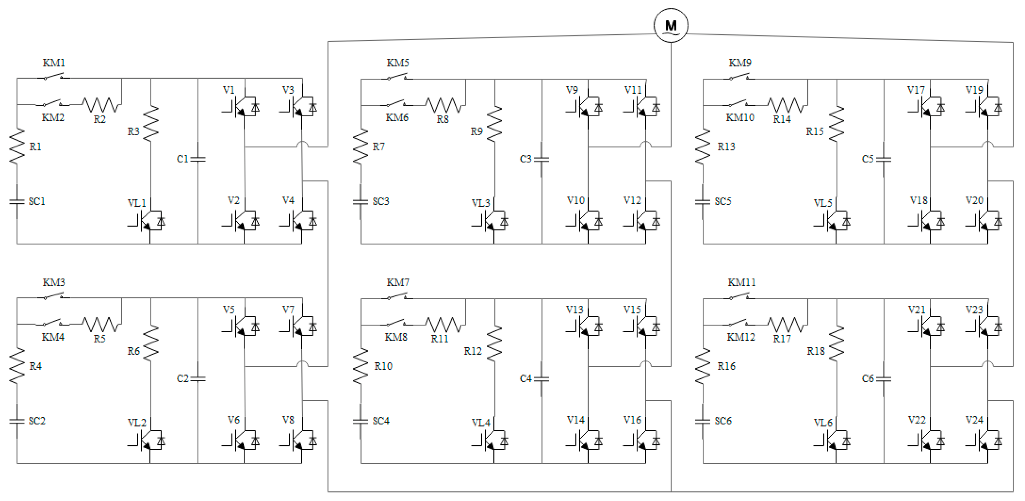
3. Calculation Method for Waveform Distortion of Variable-Frequency Current of Inverter Output

3.1. Theoretical Model of Inverter Output Variable-Frequency Current

3.1.1. Theoretical Model of Linear Variable-Frequency Current

Taking the inverter supplying power to the synchronous motor as an example, the electromagnetic torque of the motor rotor in the dq coordinate system can be expressed by:

$$T_e=\frac{3}{2}P\left({\psi }_d{i}_q-{\psi }_q{i}_d\right)$$

(19)

where P is the number of pole pairs of the permanent magnet, i_d and i_q are the currents of the d and q axes, and Ψ_d and Ψ_q are the flux linkages of the d and q axes.

If we can control i_d = 0, Equation (19) can be simplified as:

$$T_e=\frac{3}{2}P{\psi }_f{i}_q$$

(20)

where Ψ_f is the flux linkage of the magnet.

The mechanical motion equation of the motor is:

$$J\frac{d\omega }{dt}=T_e-T_L-B\omega$$

(21)

where J is the moment of inertia, ω is the mechanical angular velocity, T_L is load torque, and B is the coefficient of viscous friction.

If the motor operates in the constant acceleration stage, it is supposed to set the mechanical angular acceleration as α_m. So, ω = α_mt, and it can be deduced from Equations (20) and (21) that the q-axis current in the load-free case is:

$$i_q=\frac{2}{3}\frac{J{\alpha }_m+B{\alpha }_{m}t}{P{\psi }_f}$$

(22)

According to the principle of magnetomotive force equivalence, the coordinate transformation from two-phase rotating shafting to three-phase stationary shafting is as follows:

$$\left[\begin{array}{c}{i}_a\\ i_b\\ i_c\end{array}\right]=\sqrt{\frac{2}{3}}\left[\begin{array}{cc}\cos {\theta }_e& \cos \left({\theta }_e+\frac{\pi }{2}\right)\\ \cos \left({\theta }_e-\frac{2\pi }{3}\right)& \cos \left({\theta }_e+\frac{\pi }{2}-\frac{2\pi }{3}\right)\\ \cos \left({\theta }_e-\frac{4\pi }{3}\right)& \cos \left({\theta }_e+\frac{\pi }{2}-\frac{4\pi }{3}\right)\end{array}\right]\left[\begin{array}{c}{i}_d\\ i_q\end{array}\right]$$

(23)

where the electrical angle is: ${\theta }_e=\int {\omega }_{e}dt=\frac{1}{2}P{\alpha }_m{t}^2$.

Then, under the i_d = 0 vector control mode, the stator three-phase current of the synchronous motor in the constant acceleration stage is given by:

$$\left[\begin{array}{c}{i}_a\\ i_b\\ i_c\end{array}\right]=\frac{2}{3}\sqrt{\frac{2}{3}}\frac{J{\alpha }_m+B{\alpha }_{m}t}{P{\psi }_f}\left[\begin{array}{c}\cos \left(\frac{1}{2}P{\alpha }_m{t}^2+\frac{\pi }{2}\right)\\ \cos \left(\frac{1}{2}P{\alpha }_m{t}^2+\frac{\pi }{2}-\frac{2\pi }{3}\right)\\ \cos \left(\frac{1}{2}P{\alpha }_m{t}^2+\frac{\pi }{2}-\frac{4\pi }{3}\right)\end{array}\right]$$

(24)

It can be seen from Equation (24) that the inverter outputs a three-phase variable-frequency current to the motor stator winding.

The electrical angular speed of the motor is:

$${\omega }_e=P\omega =P{\alpha }_{m}t=2\pi f$$

(25)

where f is the current frequency.

Then, the derivative of current frequency f to time t is:

$$\frac{df}{dt}=\frac{d\left(\frac{P{\alpha }_{m}t}{2\pi }\right)}{dt}=\frac{P{\alpha }_m}{2\pi }$$

(26)

It can be seen from Equation (26) that the derivative of current frequency f to time t is constant. Therefore, the frequency of the current varies linearly.

3.1.2. Theoretical Model of Nonlinear Variable-Frequency Current

In order to make the inverter drive the synchronous motor to reach the predetermined speed in the shortest time, the inverter is controlled to output the current with the maximum amplitude all the time on the premise of ensuring the safety margin of the inverter switching devices, that is, to control the maximum value of the q-axis current to remain unchanged (i_q = I_qmax). At the same time, the d-axis current is controlled to 0 (i_d =0). The mechanical motion equation of the motor is:

$$J\frac{d\omega }{dt}=T_e-B\omega =\frac{3}{2}P{\psi }_f{I}_{qmax}-B\omega$$

(27)

It can be seen from Equation (27) that I_qmax is a constant value, and the electromagnetic torque T_e is constant. With the increase in the mechanical angular velocity ω, the friction torque Bω increases, and the total torque decreases. Therefore, the acceleration dω/dt of the motor decreases continuously.

According to Formula (27):

$$\frac{d\omega }{dt}+\frac{B}{J}\omega =\frac{3}{2}\frac{P{\psi }_f{I}_{qmax}}{J}$$

(28)

Equation (28) is a first-order nonhomogeneous linear differential equation. Its general solution is:

$$\omega =e^{-\int \frac{B}{J}dt}\left(\int \frac{3}{2}\frac{P{\psi }_f{I}_{qmax}}{J}{e}^{\int \frac{B}{J}dt}+C\right)$$

(29)

It is known that when t = 0, ω = 0. So, the solution of the equation is:

$$\omega =-\frac{3}{2}\frac{P{\psi }_f{I}_{qmax}}{B}{e}^{-\frac{B}{J}t}+\frac{3}{2}\frac{P{\psi }_f{I}_{qmax}}{B}$$

(30)

The electrical angle of the motor is:

$${\theta }_e=\int {\omega }_{e}dt=\int P\omega dt=\frac{3}{2}\frac{P^2{\psi }_f{I}_{qmax}}{B}t+\frac{3}{2}\frac{P^2{\psi }_f{I}_{qmax}J}{B^2}{e}^{-\frac{B}{J}t}-\frac{3}{2}\frac{P^2{\psi }_f{I}_{qmax}J}{B^2}$$

(31)

Then, the three-phase variable-frequency current of the stator when the acceleration of the synchronous motor continuously decreases is:

$$\left[\begin{array}{c}{i}_a\\ i_b\\ i_c\end{array}\right]=i_{qmax}\left[\begin{array}{c}\cos \left(\frac{3}{2}\frac{P^2{\psi }_f{I}_{qmax}}{B}t+\frac{3}{2}\frac{P^2{\psi }_f{I}_{qmax}J}{B^2}{e}^{-\frac{B}{J}t}-\frac{3}{2}\frac{P^2{\psi }_f{I}_{qmax}J}{B^2}+\frac{\pi }{2}\right)\\ \cos \left(\frac{3}{2}\frac{P^2{\psi }_f{I}_{qmax}}{B}t+\frac{3}{2}\frac{P^2{\psi }_f{I}_{qmax}J}{B^2}{e}^{-\frac{B}{J}t}-\frac{3}{2}\frac{P^2{\psi }_f{I}_{qmax}J}{B^2}+\frac{\pi }{2}-\frac{2\pi }{3}\right)\\ \cos \left(\frac{3}{2}\frac{P^2{\psi }_f{I}_{qmax}}{B}t+\frac{3}{2}\frac{P^2{\psi }_f{I}_{qmax}J}{B^2}{e}^{-\frac{B}{J}t}-\frac{3}{2}\frac{P^2{\psi }_f{I}_{qmax}J}{B^2}+\frac{\pi }{2}-\frac{4\pi }{3}\right)\end{array}\right]$$

(32)

The electrical angular speed of the motor is:

$${\omega }_e=P\omega =-\frac{3}{2}\frac{P^2{\psi }_f{I}_{qmax}}{B}{e}^{-\frac{B}{J}t}+\frac{3}{2}\frac{P^2{\psi }_f{I}_{qmax}}{B}=2\pi f$$

(33)

The current frequency is:

$$f=-\frac{3}{4}\frac{P^2{\psi }_f{I}_{qmax}}{\pi B}{e}^{-\frac{B}{J}t}+\frac{3}{4}\frac{P^2{\psi }_f{I}_{qmax}}{\pi B}$$

(34)

Then, the derivative of current frequency to time t is:

$$\frac{df}{dt}=\frac{3}{4}\frac{P^2{\psi }_f{I}_{qmax}}{\pi J}{e}^{-\frac{B}{J}t}$$

(35)

It can be seen from Equation (35) that the derivative of current frequency f to time t is a negative exponential power of decline. Therefore, the frequency of the current varies nonlinearly.

3.2. Waveform Distortion of Variable-Frequency Current

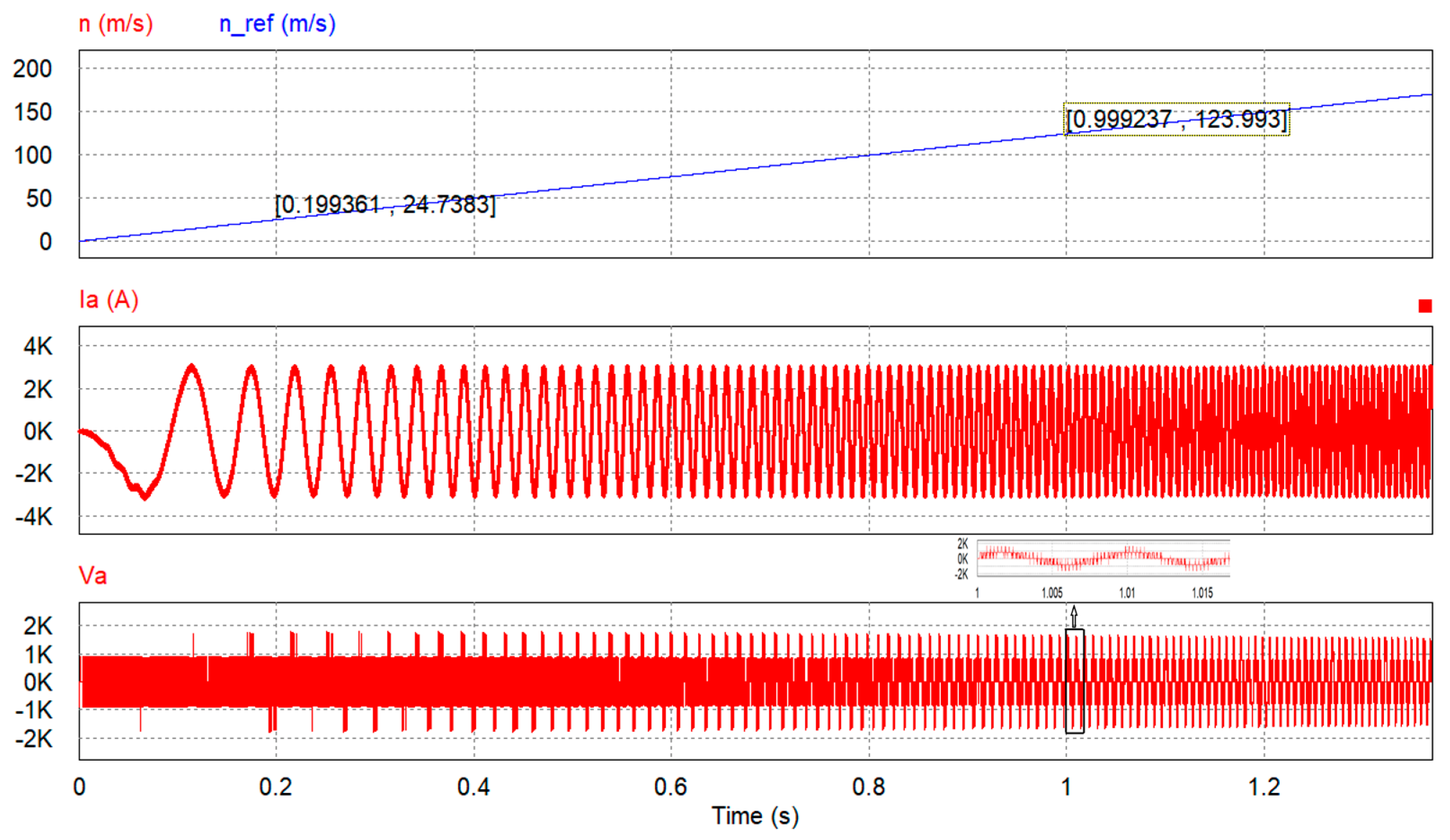
3.2.1. Waveform Distortion of Linear Variable-Frequency Current

According to Equation (24), the ideal expression of the a-phase variable-frequency current is:

$$i_a\left(t\right)=\frac{2}{3}\sqrt{\frac{2}{3}}\frac{J{\alpha }_m+B{\alpha }_{m}t}{P{\psi }_f}\cos \left(\frac{1}{2}P{\alpha }_m{t}^2+\frac{\pi }{2}\right)$$

(36)

However, due to the modulation strategy, switch dead time, digital control delay, and other reasons in the actual system, the actual current waveform is distorted, and the expression of the desired waveform needs to be obtained by nonlinear least-squares curve fitting. The subsequence i_ak (k = 1, 2, ..., m) with length m is sampled from the simulation data of i_a(t) of the synchronous motor in the constant acceleration stage as the actual waveform data, and the fitting waveform of i_ak is calculated according to curve fitting:

$$\widehat{i_a\left(t\right)}=\left(I_m+bt\right)\cos \left(c{t}^2+d\right)$$

(37)

where I_m, b, c, and d are coefficients to be calculated.

The sum of squared residuals of the a-phase current is:

$$S={\displaystyle \sum }_{k=1}^m{\left(i_{ak}-\left(I_m+b{t}_k\right)\cos \left(c{t}_k^2+d\right)\right)}^2$$

(38)

Through the nonlinear least-squares curve fitting method in Section 2.3, we can calculate I_m, b, c, and d and obtain the fitting expression of the a-phase variable-frequency current.

The rms of residuals of the a-phase variable-frequency current is:

$$RMSE=\sqrt{\frac{1}{m}{\displaystyle \sum }_{k=1}^m{\left(i_{ak}-\left(I_m+b{t}_k\right)\cos \left(c{t}_k^2+d\right)\right)}^2}$$

(39)

when the frequency changes linearly, the waveform distortion of the variable-frequency current (I_WDVF) is the ratio of the rms of residuals between the actual waveform and the fitting waveform to the rms of the variable-frequency current waveform with initial amplitude I_m:

$$I_{WDVF}=\frac{RMSE}{I_m/\sqrt{2}}\times 100\%$$

(40)

where I_m is the amplitude of the variable-frequency current.

3.2.2. Waveform Distortion of Nonlinear Variable-Frequency Current

When the acceleration of the synchronous motor decreases continuously, the theoretical expression of the a-phase variable-frequency current is:

$$i_a\left(t\right)=I_{qmax}\cos \left(\frac{3}{2}\frac{P^2{\psi }_f{I}_{qmax}}{B}t+\frac{3}{2}\frac{P^2{\psi }_f{I}_{qmax}J}{B^2}{e}^{-\frac{B}{J}t}-\frac{3}{2}\frac{P^2{\psi }_f{I}_{qmax}J}{B^2}+\frac{\pi }{2}\right)$$

(41)

The subsequence i_ak (k = 1, 2, ..., m) with length m is sampled from the simulation data of i_a(t) as the actual waveform data, and the fitting waveform of i_ak is calculated according to curve fitting:

$$\widehat{i_a\left(t\right)}=I_{qmax}\cos \left(at+b{e}^{-ct}-b+d\right)$$

(42)

where a, b, c, and d are coefficients to be calculated.

The sum of squared residuals of the a-phase current is:

$$S={\displaystyle \sum }_{k=1}^m{\left(i_{ak}-I_{qmax}\cos \left(at+b{e}^{-ct}-b+d\right)\right)}^2$$

(43)

Through the nonlinear least-squares curve fitting method in Section 2.3, we can calculate a, b, c, and d and obtain the fitting expression of the a-phase variable-frequency current.

The rms of residuals of the a-phase variable-frequency current is:

$$RMSE=\sqrt{\frac{1}{m}{\displaystyle \sum }_{k=1}^m{\left(i_{ak}-I_{qmax}\cos \left(at+b{e}^{-ct}-b+d\right)\right)}^2}$$

(44)

$$I_{WDVF}=\frac{RMSE}{I_{qmax}/\sqrt{2}}\times 100\%$$

(45)

The I_WDVF is used as the evaluation index of waveform quality of the inverter output variable-frequency current. The smaller the value of the I_WDVF, the smaller the thrust fluctuation and loss of synchronous motor, and the better the waveform quality of the variable-frequency current.

4. Simulation Verification

The simulation system of a synchronous motor driven by a cascaded H-bridge five-level inverter is built using PSIM software, as shown in Figure 1, and the specific simulation parameters are shown in

Table 1. Parameters of cascaded H-bridge five-level inverter and synchronous motor.

H-Bridge Unit			Synchronous Motor
SC1-6	Supercapacitor capacitance	17.37 F	Rs	Stator winding resistance	0.0367 Ω
	Supercapacitor voltage	912 V	Ld, Lq	d-axis and q-axis inductance	0.125 mH
	Supercapacitor internal resistance	119.7 mΩ	J	Moment of inertia	22.2 kg·m2
C1-6	Support capacitance	20 mF	B	Viscous friction coefficient	0.25 N·s/m
R1,4,7,10,13,16	Bus resistance	0.4 mΩ	Ψf	Flux linkage	0.91 Wb
V1-24	IGBT rated voltage	1700 V	P	Number of pole pairs	2
	IGBT rated current	3600 A	τ	Polar distance	0.54 m
			Pn	Rated power	4.5 MW

.

4.1. Waveform Quality Evaluation of Constant-Frequency Current

Given the speed curve to be the step input curve, after reaching the steady state, the stator current of the motor is a three-phase constant-frequency sinusoidal current, which is 80 Hz. The inverter adopts the carrier-phase-shifted sinusoidal pulse-width modulation (CPS-SPWM), and the triangular carrier frequency (f_c) is 1 kHz. Based on the above simulation conditions and parameter settings in Table 1, the inverter output current response at a constant frequency can be obtained through PSIM simulation.

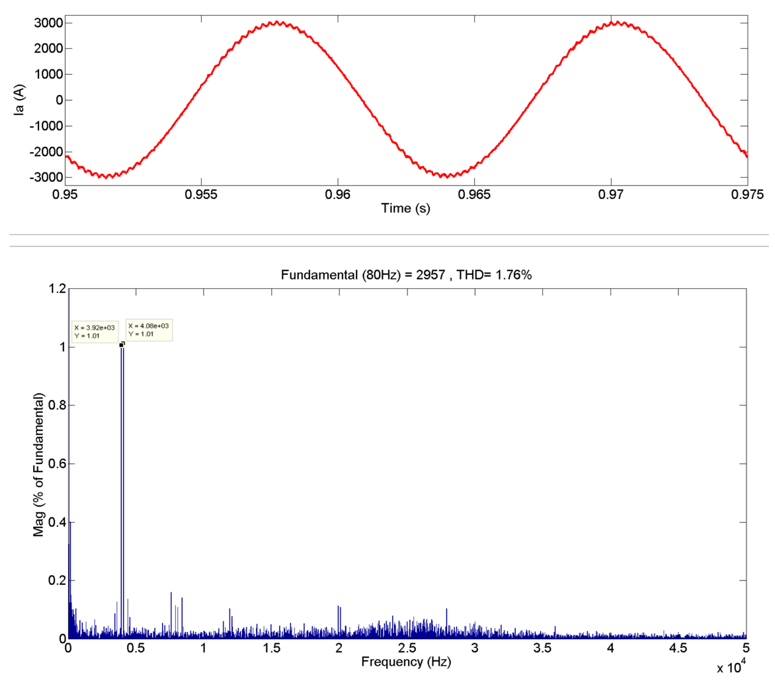
4.1.1. Waveform Quality Evaluation of Constant-Frequency Current for Higher Oversampling

When a higher oversampling (f_s = 100 kHz) is adopted, two cycles of data points of the a-phase current are sampled. The sampling points are imported into the MATLAB workspace, and the FFT analysis results are obtained by the FFT tool, as shown in Figure 2. It can be seen from Figure 2 that the fundamental frequency (f) of the a-phase current is 80 Hz, and the current THD (I_THD) is 1.76%. The inverter output a-current contains rich high-order harmonics. The highest harmonic frequency of the current sampling signal is 50 kHz. These high-order harmonics are mainly distributed at 4 nf_c + mf frequencies, where f_c = 1 kHz, f = 80 Hz, n = 1, 2, 3, ..., and m = ± 1, ± 3, ± 5, .... The higher sampling frequency ensures the accuracy of discrete signals in the time domain and the frequency domain.

For the same a-phase current sampling points as Figure 2, the fitting expression to be solved is customized as $i_a=I_m\cos \left(bt+c\right)$ by the MATLAB curve fitting tool. The sampling points are fitted by the nonlinear least-squares method, and the fitting results are shown in Figure 3. It can be seen from Figure 3 that the black dots are the sampling points of the a-phase current waveform. The blue line is the fitting curve. The RMSE is 36.95, and the fitting expression of the a-phase current is $i_a=2957\cos \left(503.2t-4.457\right)$.

According to the definition of WD of periodic signals, the WD of a-phase constant-frequency current for higher oversampling is $I_{WD}=\frac{RMSE}{I_m/\sqrt{2}}\times 100\%=\frac{36.95}{2957/\sqrt{2}}\times 100\%=1.76\%$.

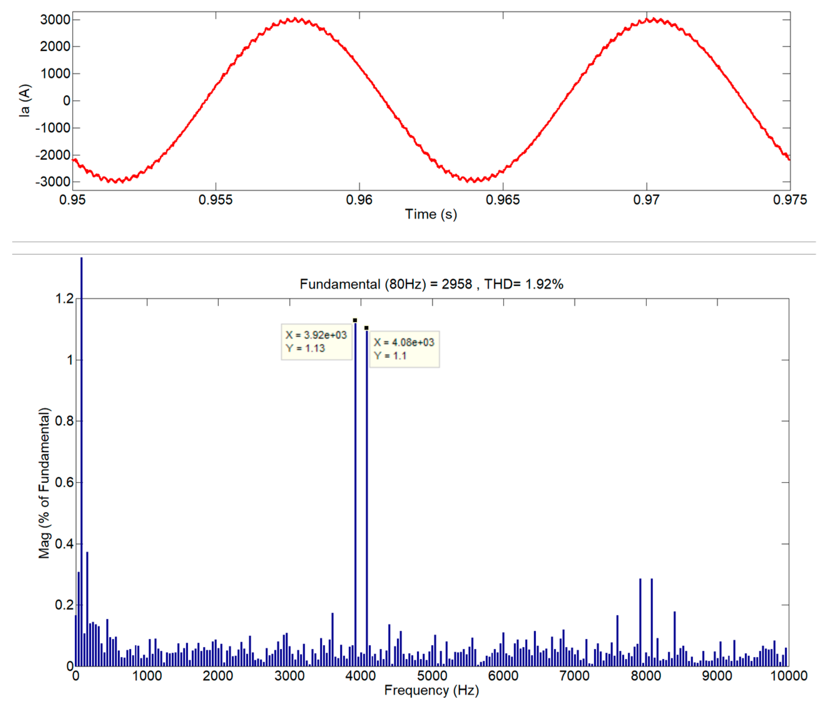
4.1.2. Waveform Quality Evaluation of Constant-Frequency Current for Lower Oversampling

For the same constant-frequency current as Section 4.1.1, when a lower oversampling (f_s = 20 kHz) is adopted, two cycles of data points of the a-phase current are sampled. The sampling points are imported into the MATLAB workspace, and the FFT analysis results are obtained by the FFT tool, as shown in Figure 4. It can be seen from Figure 4 that the fundamental frequency of the a-phase current is 80 Hz, and the current THD (I_THD) is 1.92%. In fact, the a-phase current contains rich high-order harmonics. However, the lower sampling frequency results in the highest harmonic frequency of the current sampling signal being only 10 kHz, which leads to the appearance of spectrum aliasing and error of measurement.

For the same a-phase current sampling points as Figure 4, the fitting expression to be solved is customized as $i_a=I_m\cos \left(bt+c\right)$ by the MATLAB curve fitting tool. The sampling points are fitted by the nonlinear least-squares method, and the fitting results are shown in Figure 5. It can be seen from Figure 5 that the black dots are the sampling points of the a-phase current waveform. The blue line is the fitting curve. The RMSE is 40.29, and the fitting expression of the a-phase current is $i_a=2958\cos \left(503.2t-4.456\right)$.

According to the definition of the WD of periodic signals, the WD of the a-phase constant-frequency current for lower oversampling is $I_{WD}=\frac{RMSE}{I_m/\sqrt{2}}\times 100\%=\frac{40.29}{2958/\sqrt{2}}\times 100\%=1.92\%$.

In conclusion, the comparison results of the waveform quality evaluation of the constant-frequency current at different sampling frequencies are obtained by curve fitting and FFT, as shown in

Table 2. Comparison of waveform quality evaluation of constant-frequency current at different sampling frequencies.

	Curve Fitting			FFT
Sampling Frequency	Fitting Expression	RMSE	IWD	ITHD
fs = 100 kHz	$i_a=2957\cos \left(503.2t-4.457\right)$	36.95	1.76%	1.76%
fs = 20 kHz	$i_a=2958\cos \left(503.2t-4.456\right)$	40.29	1.92%	1.92%

.

For the same constant-frequency current waveform, it can be seen from Table 2 that when a higher oversampling (f_s = 100 kHz) is adopted, the total harmonic distortion (I_THD) of the current is 1.76% through FFT simulation in the frequency domain, and the current waveform distortion (I_WD) is 1.76% through the time-domain curve fitting simulation. When a lower oversampling (f_s = 20 kHz) is adopted, the I_THD obtained by the FFT method is 1.92%, and the I_WD obtained by the curve fitting method is 1.92%. The size of the waveform quality evaluation indicators I_THD and I_WD obtained by the two methods is basically consistent with the theoretical analysis results in Section 2.2, which verifies the equivalence of the two methods. Two full cycles of data points are sampled to meet the synchronization of sampling frequency and signal frequency, which is conducive to reducing spectrum leakage. However, when the sampling frequency is low, the number of sampling points is small. Spectrum aliasing and the fence effect are more obvious, which leads to the increase in I_THD and I_WD. Therefore, in order to reduce the impact of spectrum aliasing and the fence effect, a higher sampling frequency of 100 kHz is adopted in Section 4.2 and Section 4.3.

4.2. Waveform Quality Evaluation of Linear Variable-Frequency Current

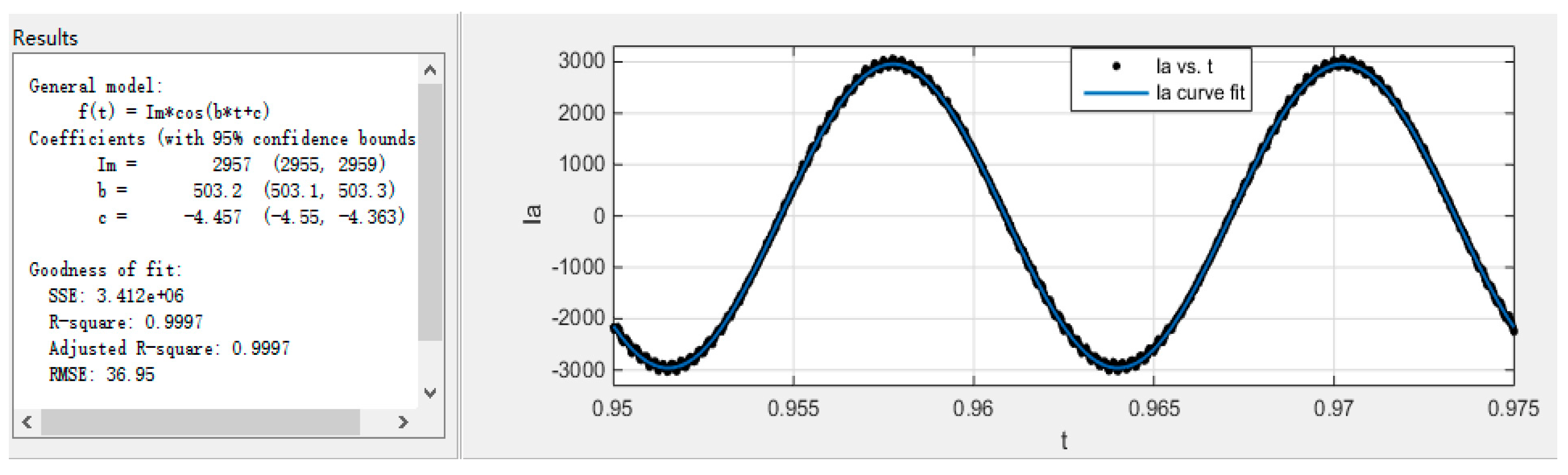
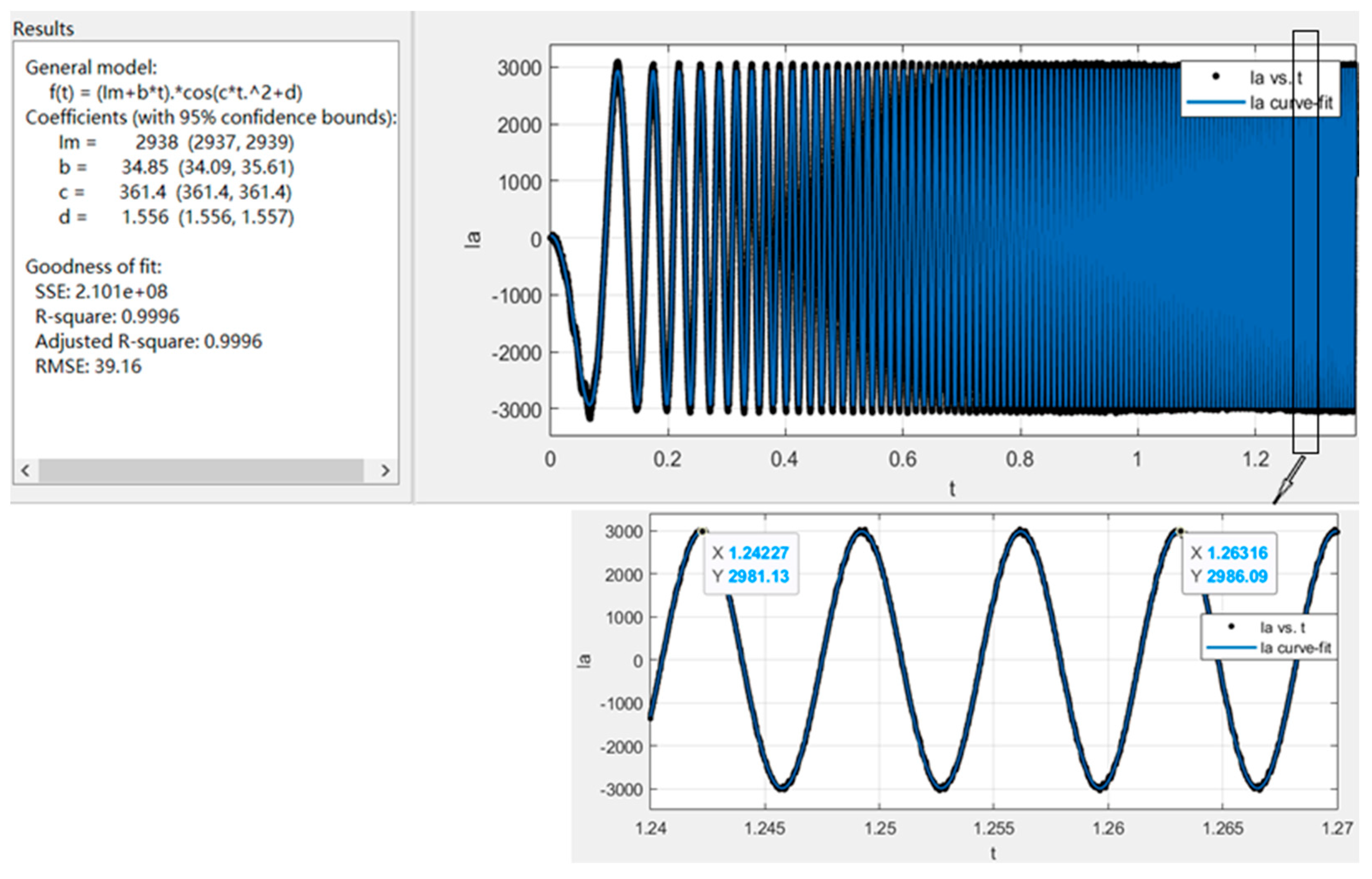
4.2.1. Simulation Calculation of I_WDVF Based on Curve Fitting

Different from Section 4.1, the given speed of the motor is a slope curve. The speed is accelerated from 0 to 170 m/s at 1.37 s, and the frequency is linearly increased from 0 to 157.4 Hz. In this process, the inverter outputs a variable-frequency current. The simulation step is set to 10 μs. Based on the above simulation conditions and the parameter settings in Table 1, the motor is driven by the cascaded H-bridge five-level inverter. The curves of the motor speed, inverter a-phase variable-frequency current, and voltage are obtained through PSIM simulation, as shown in Figure 6. It can be seen from Figure 6 that the motor speed changes linearly. Therefore, the current frequency also varies linearly.

The sampling points of the a-phase variable-frequency current are imported into MATLAB. According to the ideal expression type of the variable-frequency current of the motor in the constant acceleration stage, the expression of the fitting function is customized as $i_a=\left(I_m+bt\right)\cos (c{t}^2+d)$ by the curve fitting tool. The sampling points are fitted by the nonlinear least-squares method. The fitting results and local amplified waveform are shown in Figure 7.

It can be seen from Figure 7 that the black spots are the sampling points of the a-phase variable-frequency current. The blue line is the fitting curve, and the RMSE is 39.16. The fitting expression of the a-phase variable-frequency current is $i_a=\left(2938+34.85t)\cos (361.4t^2+1.556\right)$. The R-square reaches 0.9996. The closer the R-square is to 1, the better the fitting effect, which shows that the accuracy of the fitting expression of the variable-frequency current is high. Finally, the I_WDVF is obtained according to its definition:

$$I_{WDVF}=\frac{RMSE}{I_m/\sqrt{2}}\times 100\%=\frac{39.16}{2938/\sqrt{2}}\times 100\%=1.88\%$$

4.2.2. Approximate Estimation of I_WDVF with Average Value of Constant-Frequency I_THD

According to the principle of the variable voltage and variable-frequency speed regulation of the motor, the speed is accelerated from 0 to 170 m/s, the current frequency is linearly increased from 0 to 157.4 Hz, and the current frequency is linear with the speed. In the process of constant acceleration, the current frequency changes all the time, so the THD of the variable-frequency current in the whole process of acceleration cannot be directly calculated by the FFT method.

Since the frequency changes linearly in the constant acceleration process, the I_WDVF is approximately estimated by calculating the average value of the I_THD within the variable-frequency range. The steady-state operating conditions of the motor at different constant frequencies are simulated in turn, then the I_THD at this frequency is calculated, and finally, the average value of the I_THD corresponding to all frequency points is calculated. The simulation step is set to 10 μs. Based on the above ideas and the parameter settings in Table 1, the given speed is set as different step curves (corresponding to different frequencies) in the simulation model. Driven by the cascaded H-bridge five-level inverter, the motor is operated under steady-state conditions of the given speed, and the a-phase I_THD corresponding to different constant frequencies is successively simulated, as shown in

Table 3. A-phase I_THD corresponding to different frequencies.

f(Hz)	ITHD	f(Hz)	ITHD	f(Hz)	ITHD
10	1.72%	60	1.79%	110	1.63%
20	1.78%	70	1.79%	120	1.62%
30	1.79%	80	1.76%	130	1.64%
40	1.78%	90	1.78%	140	2.09%
50	1.78%	100	1.67%	150	2.20%

.

From Table 3, it can be calculated that the average value of the I_THD at different frequencies in the whole process of variable frequency from 10 to 150 Hz is 1.79%. The modulation method is carrier-phase-shifted sinusoidal pulse-width modulation (CPS-SPWM), the carrier frequency is 1 kHz, and when the fundamental frequency becomes larger, the carrier wave ratio becomes smaller, resulting in a larger THD. When the fundamental frequency becomes larger, the modulation ratio becomes larger, resulting in the THD becoming smaller first and then larger. When the fundamental frequency is 140 and 150 Hz, the modulation ratio gradually approaches 1, resulting in an increase in THD. The interaction of the two causes leads to an increase in THD at the last two frequencies. The disadvantages are that the I_THD needs to be calculated for different frequency points one by one, and the amount of simulation calculation is large.

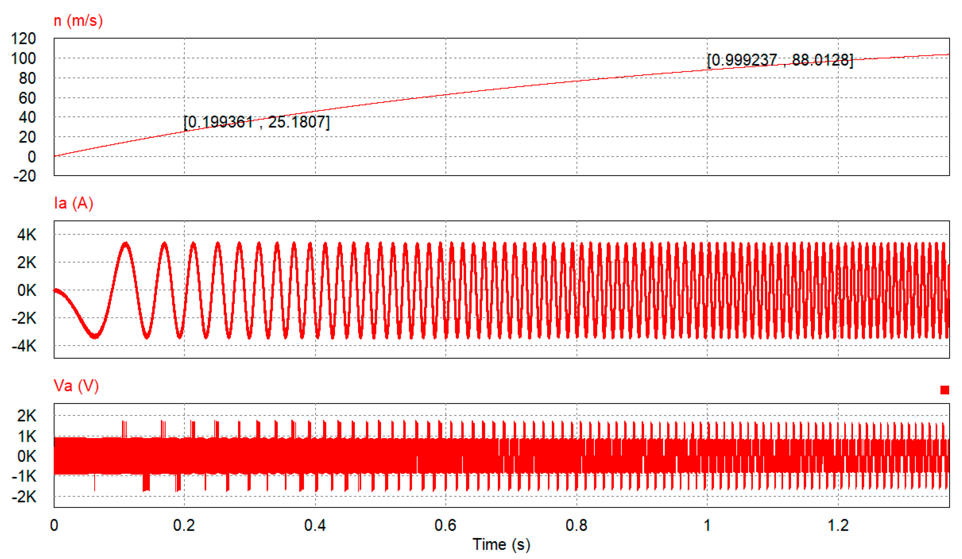
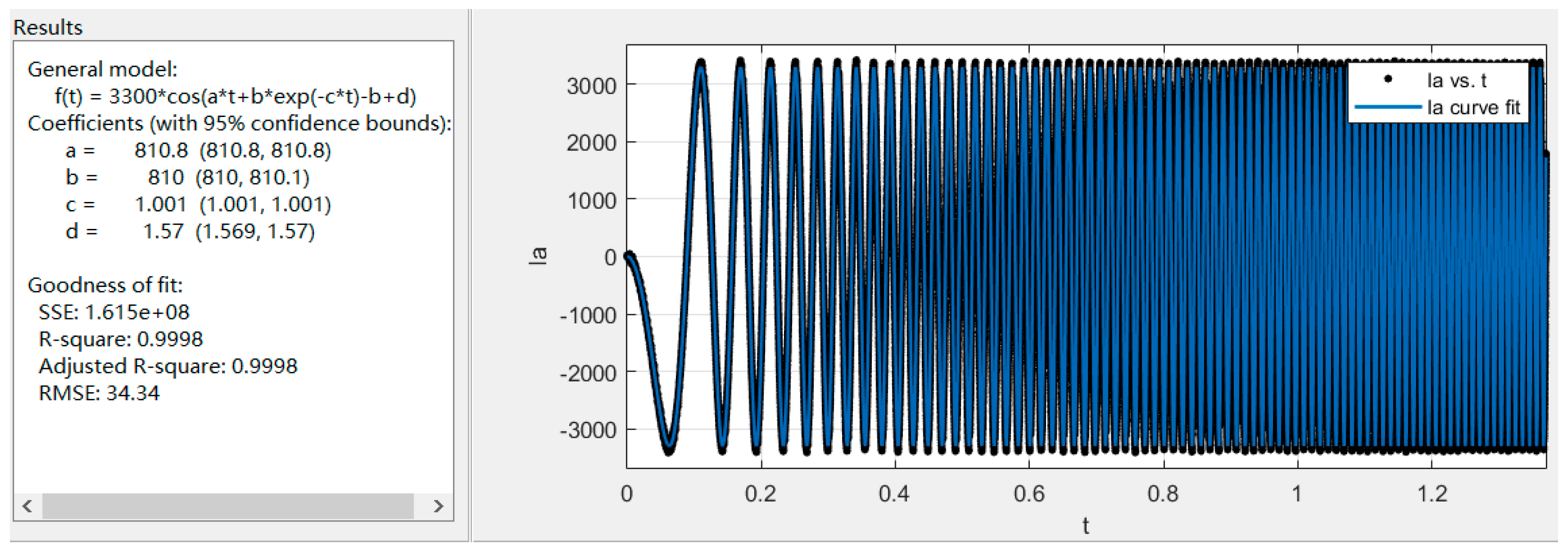
4.3. Waveform Quality Evaluation of Nonlinear Variable-Frequency Current

Different from Section 4.2, the given motor q-axis current I_qmax = 3300 A remains unchanged, allowing the motor to accelerate to the preset speed in the shortest time under the safety limit of the inverter IGBT. In this process, the inverter outputs a variable-frequency current. In order to clearly see the nonlinear change in motor speed, increase the friction coefficient B of the motor in Table 1 to 22.2 N·s/m. Based on the above simulation conditions and the parameter settings in Table 1, the motor is driven by a cascaded H-bridge five-level inverter. The curves of the motor speed, inverter a-phase variable-frequency current, and voltage are obtained through PSIM simulation, as shown in Figure 8. It can be seen from Figure 8 that the motor speed changes nonlinearly. Therefore, the current frequency also varies nonlinearly.

The waveform data of the a-phase variable-frequency current is imported into MATLAB. According to the theoretical model of the nonlinear variable-frequency current, the expression of the fitting function is customized as $i_a=3300\cos \left(at+b{e}^{-ct}-b+d\right)$ by the curve fitting tool. The waveform data are fitted by the nonlinear least-squares method, and the fitting results are shown in Figure 9.

It can be seen from Figure 9 that the black spots are the sampling points of the a-phase nonlinear variable-frequency current. The blue line is the fitting curve, and the RMSE is 34.34. The fitting expression of the a-phase variable-frequency current is $i_a=3300\cos \left(810.8t+810e^{-1.001t}-810+1.57\right)$. The R-square reaches 0.9998, which shows that the accuracy of the fitting expression of the variable-frequency current is high. Finally, the I_WDVF is obtained according to its definition: $I_{WDVF}=\frac{RMSE}{I_{qmax}/\sqrt{2}}\times 100\%=\frac{34.34}{3300/\sqrt{2}}\times 100\%=1.47\%$.

In conclusion, when the sampling frequency is 100 kHz, the comparison results of the waveform quality evaluation of the inverter output constant-frequency current and variable-frequency current are obtained by curve fitting and FFT, as shown in

Table 4. Comparison of waveform quality evaluation of inverter output constant-frequency current and variable-frequency current.

	Curve Fitting			FFT
Constant-frequency current	Fitting Expression	RMSE	IWD	ITHD
	$i_a=2957\cos \left(503.2t-4.457\right)$	36.95	1.76%	1.76%
	Fitting expression	RMSE	IWDVF	Average value of ITHD
Linear variable-frequency current	$i_a=\left(2938+34.85t)\cos (361.4t^2+1.556\right)$	39.16	1.88%	1.79%
Nonlinear variable-frequency current	$i_a=3300\cos \left(810.8t+810e^{-1.001t}-810+1.57\right)$	34.34	1.47%

.

It can be seen from Table 4 that for the waveform quality evaluation of the constant-frequency current, the I_THD obtained by FFT is 1.76%, and the I_WD obtained by curve fitting is 1.76%. It is verified that the I_WD obtained by curve fitting is correct as the current waveform quality evaluation index.

For the waveform quality evaluation of the linear variable-frequency current, the I_WDVF obtained by curve fitting is 1.88%, and the average value of the I_THD of the variable-frequency current obtained by FFT is 1.79%. The feasibility of the I_WDVF obtained by nonlinear least-squares curve fitting is verified. Because FFT cannot correctly solve the THD of the variable-frequency current, we use the average value of the I_THD of the constant-frequency current for estimation. The I_WDVF is close to the average value of the I_THD, which verifies that the time-domain curve fitting method proposed in this paper is reasonable to solve the I_WDVF.

For the waveform quality evaluation of the nonlinear variable-frequency current, the I_WDVF obtained by curve fitting is 1.47%. Because the inverter continuously outputs a variable-frequency current with a maximum amplitude of 3300 A, the denominator used for calculating the I_WDVF is large. At the same time, the modulation ratio of the inverter with a nonlinear variable-frequency current is higher than that of the inverter with a linear variable-frequency current. Therefore, the waveform distortion of the nonlinear variable-frequency current is less than that of the linear variable-frequency current. This kind of nonlinear variable-frequency current is ubiquitous in electromagnetic launch, aerospace electromagnetic launch, and other fields. The curve fitting method can reasonably solve the distortion degree of the nonlinear variable-frequency current, which verifies that the curve fitting method is universal in solving the distortion of the variable-frequency current.

5. Conclusions

Aiming at the variable-frequency application of high-power inverters in the field of electromagnetic launch, a method for evaluating the waveform quality of the inverter output variable-frequency current based on the I_WDVF is proposed. This method can obtain the fitting expression of the variable-frequency current through nonlinear least-squares curve fitting in the time domain, and calculate the I_WDVF as the index for evaluating waveform quality. For constant-frequency current, the I_THD obtained by the FFT method is the same as the I_WD obtained by the curve fitting method, which verifies the equivalence of the two methods under the condition of full-period sampling. The influence of different sampling frequencies on the I_WD and I_THD is compared. The higher the sampling frequency, the more sampling points, and the more accurate the results. For linear variable-frequency current, the I_WDVF obtained by the time-domain curve fitting method is close to the average value of the I_THD obtained by the frequency-domain FFT method, indicating that the I_WDVF obtained by the time-domain curve fitting method is reasonable. For nonlinear variable-frequency current waveforms, the curve fitting method can also calculate the I_WDVF. This shows that the curve fitting method can reasonably calculate the I_WDVF of different types of variable-frequency currents on the premise that the frequency function is known. The method proposed in this paper solves the problem that frequency-domain FFT cannot directly solve the THD of the variable-frequency current. It can quickly compare the effects of different modulation strategies on the inverter output variable-frequency current waveform quality, and provide a basis for the optimal design of modulation strategy aiming at the optimal waveform quality of the variable-frequency current.

References

1. Zhang, G.; Yan, Y.; Wang, Z.; Xia, C. An Analytical Evaluation Method for Output Waveform Quality of Three-level Inverters Based on the Amplitude of the Mean Current Ripple Vector. Proc. CSEE 2017, 37, 6410–6417. (In Chinese) [Google Scholar]
2. Beig, A.R.; Kanukollu, S.; Al Hosani, K.; Dekka, A. Space-vector-based synchronized three-level discontinuous PWM for medium-voltage high-power VSI. IEEE Trans. Ind. Electron. 2014, 61, 3891–3901. [Google Scholar] [CrossRef]
3. Kelly, J.; Aldaiturriaga, E.; Ruiz-Minguela, P. Applying international power quality standards for current harmonic distortion to wave energy converters and verified device emulators. Energies 2019, 12, 3654. [Google Scholar] [CrossRef] [Green Version]
4. Xiao, X.; Collin, A.J.; Djokic, S.Z.; Yanchenko, S.; Möller, F.; Meyer, J.; Langella, R.; Testa, A. Analysis and Modelling of Power-Dependent Harmonic Characteristics of Modern PE Devices in LV Networks. IEEE Trans. Power Deliv. 2017, 32, 1014–1023. [Google Scholar] [CrossRef] [Green Version]
5. IEEE Standard 519-2014; IEEE 519 Recommended Practice and Requirements for Harmonic Control in Electric Power Systems. IEEE: New York, NY, USA, 2014.
6. IEEE Std. 1547-2018; Standard for Interconnection and Interoperability of Distributed Energy Resources with Associated Electric Power Systems Interfaces. IEEE: New York, NY, USA, 2018.
7. Hu, Z.; Zhang, Y.; Yin, J.; Liu, F. Overview of Maglev electromagnetic boost launch technology for aerospace vehicles. Winged Missile 2016, 12, 54–59. [Google Scholar]
8. Ma, W.; Xiao, F.; Nie, S. Applications and Development of Power Electronics in Electromagnetic Launch System. Trans. China Electrotech. Soc. 2016, 31, 1–10. [Google Scholar]
9. Ma, W.; Lu, J. Electromagnetic Launch Technology. J. Natl. Univ. Def. Technol. 2016, 38, 1–5. [Google Scholar]
10. Fair, H.D. Advances in Electromagnetic Launch Science and Technology and Its Applications. IEEE Trans. Magn. 2009, 45, 225–230. [Google Scholar] [CrossRef]
11. Basir, M.S.S.M.; Ismail, R.C.; Yusof, K.H.; Katim, N.I.A.; Isa, M.N.M.; Naziri, S.Z.M. An implementation of Short Time Fourier Transform for Harmonic Signal Detection. J. Phys. Conf. Ser. 2020, 1755, 012013. [Google Scholar] [CrossRef]
12. Arranz-Gimon, A.; Zorita-Lamadrid, A.; Morinigo-Sotelo, D.; Duque-Perez, O. A Review of Total Harmonic Distortion Factors for the Measurement of Harmonic and Interharmonic Pollution in Modern Power Systems. Energies 2021, 14, 6467. [Google Scholar] [CrossRef]
13. Ma, L.; Zhou, L.; Wang, L.; Zhang, H. Adaptive harmonic detection algorithm based on fourier series. Electron. Meas. Technol. 2016, 39, 34–37. [Google Scholar]
14. Zhao, Y.; Huo, K.; Chen, Z. Research and Implementation of AC Distortion Factor Measurement. Electr. Meas. Instrum. 2014, 51, 74–79. [Google Scholar]
15. Liang, Z.; Zhu, J. The Correction of the Influence of Quantization Error to the Evaluation of the Distortion of Periodic Signal. Chin. J. Sci. Instrum. 2000, 21, 640–643. [Google Scholar]
16. Martinek, R.; Rzidky, J.; Jaros, R.; Bilik, P.; Ladrova, M. Least mean squares and recursive least squares algorithms for total harmonic distortion reduction using shunt active power filter control. Energies 2019, 12, 1545. [Google Scholar] [CrossRef]
Figure 1. Simulation system of synchronous motor driven by cascaded H-bridge five-level inverter.
Energies 15 07594 g001
Figure 2. FFT analysis results of constant-frequency current for higher oversampling.
Energies 15 07594 g002
Figure 3. Curve fitting results of a-phase current for higher oversampling.
Energies 15 07594 g003
Figure 4. FFT analysis results of constant-frequency current for lower oversampling.
Energies 15 07594 g004
Figure 5. Curve fitting results of constant-frequency current for lower oversampling.
Energies 15 07594 g005
Figure 6. Curve of motor speed and a-phase linear variable-frequency current.
Energies 15 07594 g006
Figure 7. Curve fitting results of a-phase linear variable-frequency current.
Energies 15 07594 g007
Figure 8. Curves of motor speed, inverter a-phase variable-frequency current, and voltage.
Energies 15 07594 g008
Figure 9. Curve fitting results of a-phase nonlinear variable-frequency current.
Energies 15 07594 g009