Abstract
The large-scale integration of variable renewable energy sources into the energy system presents techno–economic challenges. Long–term energy system optimization models fail to adequately capture these challenges because of the low temporal resolution of these tools. This limitation has often been addressed either by direct improvements within the long–term models or by coupling them to higher resolution power system models. In this study, a combined approach is proposed to capitalize on the advantages and overcome the disadvantages of both methods. First, the temporal resolution of an energy model was enhanced by approximating the joint probability of the electricity load and the supply of intermittent sources. Second, the projected electricity mix was simulated by a power model at an hourly resolution. This framework was used to analyze mid–century deep decarbonization trajectories for Colombia, subject to future uncertainties of hydroclimatic variability and the development of the bioeconomy. The direct integration method is found to consistently reduce the overestimation of the feasible penetration of VRES. However, its impact is marginal because of its inability to assess the short–term operation of the power system in detail. When combined with the soft–linking method, the reliable operation of the power system is shown to incur an additional overhead of 12–17% investment in flexible generation capacity, 2–5% of the annual energy system cost, and a 15–27% shortfall in achieving the aspired GHG mitigation target. The results obtained by combining both methods are found to be closer to the global optimum solution than using either of these methods individually.
1. Introduction
The transition towards a low-carbon supply of electricity is a key cost-effective measure to stabilize the concentration of greenhouse gases (GHG) in the atmosphere [1]. Solar and wind power are projected to make an increasing contribution to the supply of low-carbon electricity throughout the 21st century [2]. However, the intermittency and limited predictability of these variable renewable energy sources (VRES) pose technical and economic challenges to their large-scale integration into the energy system [3]. These challenges have often been insufficiently captured by long-term planning models because of the low temporal, spatial, and technical resolution of these tools. Conversely, dedicated power system models can simulate the operation of the power system at high resolutions, although they often disregard the long-term evolution of the system or its interaction with other energy sectors [4].
State of the art approaches to address the challenges associated with the large-scale penetration of VRES in long-term planning models include direct integration methods, that is, improving the representation of VRES integration in these models, and soft-linking them to power system models [5]. Soft-linking methods are either uni- or bi-directional. Uni-directional methods verify the robustness of the results of the long-term planning models by simulating these results in power system models. However, they do not enhance the optimality of the solution. Bi-directional methods with iterative linking can address this shortfall, although it is a complex procedure and its convergence towards optimality is not guaranteed. Direct integration techniques in long-term planning models allow for increased optimality without the need for iterations. However, they fail to assess the short-term reliability of the power system operation. While the differences between these methods have been discussed in reviews, little research has been done to compare them for the same case study [4].
Combining direct integration and soft-linking methods could overcome the limitations of each and assess their convergence towards optimality. To demonstrate this approach, Colombia was identified as a case study, where the role of VRES is likely to be influenced by the development of hydropower and bioenergy, which can be variable and uncertain.
Case Study
Colombia exhibits a low carbon intensity of electricity production [6] because of the high share of hydropower in the capacity mix (approximately 70%) [7]. The predominance of hydro exposes the power system to the impacts of hydroclimatic variability. These impacts include long-term alterations in mean-state rainfall induced by climate change [8] and extreme events of drought and flood driven by El Niño Southern Oscillation (ENSO) [9]. Dealing with El Niño episodes has been shown to augment the use of reserve coal and natural gas capacity, causing spikes in spot electricity prices [10] and increased carbon intensity of electricity [11].
Global circulation models (GCMs) of the 21st century climate have not agreed on the direction or magnitude of impact in the case of Colombia for the steady long-term supply of hydropower [12] or for the frequency and amplitude of extreme ENSO anomalies [13]. Medium estimates of the mean impact across various GCM scenarios are projected to be a 2–4% net loss of hydropower by the end of the century [14], whereas severely dry conditions could lead to a 13–15% loss by mid-century [15].
Without sustained measures to contain Colombia’s GHG emissions, and given the abundance of coal reserves [16] and the expected demand growth, fossil fuels are projected to be the main substitute for hydropower [17,18]. In terms of policy, the government has recently increased the ambition of its nationally determined contribution (NDC) to the Paris Climate Agreement, with the aim of curbing 51% of the total projected baseline emissions by 2030 [19]. Finding a balance between climate change mitigation and energy security will require diversification of the energy mix towards the development of low carbon alternatives to hydropower [20].
The prospects of a mid-century deep decarbonization of the Colombian energy system have been explored by two families of models. The first includes top-down computational general equilibrium (CGE) models (MEG4C and Phoenix) and integrated assessment models (IAMs), whereby Colombia is represented as a separate region (GCAM and TIAM–ECN) [15,17,18]. These tools could effectively capture system-wide feedbacks of the global economy, including the influence of climate policies beyond national borders, the role of international trade of agricultural and fossil fuel commodities, and the dynamics between energy and land use [18]. However, the coarse temporal and technical resolution of these tools limits their capacity to address the complex role of biomass [21,22,23].
The second family comprises bottom up energy system optimization models (ESOMs). Younis et al. [24] developed a detailed representation of biomass value chains for the Colombian energy system, including advanced biorefinery, bioenergy combined with carbon capture and storage (BECCS), and (bio)chemicals options. This framework is referred to as TIMES–CO–BBE (an offspring of MARKAL Colombia [25,26]). While this model can address the role of biomass better than CGE models and IAMs, it has not considered the impact of hydroclimatic variability on Colombia’s energy planning, which Arango–Aramburo et al. [15] found to be non-trivial. Moreover, the temporal, technical, and spatial granularity of both model families is insufficient in addressing the systemic integration of VRES [27,28].
These limitations have been partially addressed by using dedicated power system models of high temporal and/or spatial resolution, such as EnergyPLAN [29] and IRENA FlexTool [30]. These studies evaluated the operational flexibility of the power system by 2030 subject to the high penetration of VRES and in the case of an extreme El Niño drought event. However, these tools relied on exogenous projections of power capacity and demand and ignored the dynamic interaction between the power sector and other energy demand sectors, for example, for electric mobility.
By soft-linking an ESOM to a dedicated power model, Lap et al. [31] analyzed deep decarbonization trajectories for Brazil by 2050, considering the variability of hydro and biomass resources and the dynamic demand for electric mobility. They found that the ESOM underestimated the capacity investment needed for reliable operation of the system by an average of 7%.
In this study, a combined approach using direct integration and soft-linking methods to analyze the large-scale integration of VRES is demonstrated. First, through the direct integration in an ESOM, the use of conventional stylized time slices is compared with an alternative enhanced stylization to approximate the joint probability of electricity load and VRES supply. Second, a power model is used to simulate the operation of the capacity profile determined by the ESOM at an hourly resolution. Accordingly, the mismatch in the capacity requirement to guarantee a reliable system operation is estimated. Finally, the implications on the cost and emissions of the energy system are quantified. This approach is applied to mid-century deep decarbonization trajectories of the Colombian energy system. Scenarios reflecting uncertainties of hydroclimatic variability and the availability of biomass for advanced applications of the bioeconomy are analyzed.
2. Methods and Data
Figure 1 illustrates an overview of the methodological setup of this analysis, which is divided into three main parts.
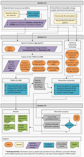
Figure 1.
Schematic overview of the modeling framework, adapted from Lap et al. [31].
The middle part represents the core of the modelling framework, namely the ESOM and power model involved in the analysis. Section 2.1 describes the underlying methods, input data, and assumptions of these models.
A special type of input data is the electricity supply and demand patterns (Figure 1, upper part). Section 2.2 addresses the analysis and profiling of spatio–temporal patterns for intermittent VRES supply (solar and wind) and electricity demand and their aggregation into stylized time slices by using a conventional and a direct integration method. It also addresses the respective baseline patterns for hydropower supply and future scenarios for hydroclimatic variability.
Finally, the lower part of Figure 1 introduces the steps applied to perform a mismatch analysis in a given scenario and the type of output indicators. Section 2.3 describes in detail the modeling steps and the organization of the scenario analysis.
2.1. Energy and Power Models
The ESOM and power system models used in this analysis are TIMES–CO–BBE and PowerPlan Colombia, respectively (Table 1). Their main features are further described in Section 2.1.1 and Section 2.1.2, respectively.

Table 1.
Main differences between the energy system and power system models used in the analysis.
2.1.1. TIMES–CO–BBE Energy System Optimization Model
MARKAL–TIMES computes least cost pathways of investment in resources and conversion technologies to meet the total energy demand (TIMES–CO–BBE covers power, fuels, heat, and chemicals) subject to system constraints [36]. The demand is determined by exogenous socio-economic drivers of energy services, for example, lighting, cooking, heating/cooling, and machine drive in four main sectors, namely, commercial and others, industrial, residential, and transport and also the demand for base chemicals, edible sugars, and oils, which are relevant for the bioeconomy. The main constraints include techno-economic learning rates and operational limits of technologies, the availability and cost of resource extraction and/or trade, emission mitigation target, and the subsurface storage potential of carbon dioxide [24] (see Supplementary S1).
The model was calibrated to the national energy balance in 2015 with a time horizon until 2050 in steps of five-year periods. Future uncertainties of technological learning and demand were represented by three projections following the Shared Socioeconomic Pathways SSP1–3 scenario analysis framework [37]. Climate change mitigation policies were analyzed in the model by means of emission caps which are based on Colombia’s NDC 2030 pledges to the Paris Agreement, and further extrapolated to 2050 [38]. The demand for electricity was endogenously determined by the demand for energy services. In this way, electricity could compete with other energy carriers, such as biomass, fossil fuels, and hydrogen. More details of the model are published elsewhere [24].
A key advantage of TIMES–CO–BBE is its comprehensive representation of biomass value chains in the energy system. Mid-century decarbonization studies have drawn divergent conclusions on the role of bioenergy in Colombia [15,17]. One of the critical factors governing this role is the availability of land for the sustainable production of dedicated energy crops [18]. To capture this dynamic, the model included a simplified land use module with possibilities to valorize sugar, oil, and lignocellulosic crops, next to agricultural and forestry residues, and animal manure.
Through this module, two scenarios of land use policy were formulated, covering a wide spectrum of biomass resource availability. The BioLo scenario was based on the continuation of current land use patterns, where scant land can be available for the sustainable production of bioenergy crops. The BioHi scenario was based on the ambitious upscaling of sustainable intensification of agricultural and livestock practices, for example, agroforestry systems, which could enhance land availability for biomass [39]. These scenarios were compared by Younis et al. [24] without addressing the system integration challenges of VRES or the impact of hydroclimatic variability. In the present study, these factors were considered.
2.1.2. PowerPlan Power System Simulation Model
PowerPlan is an interactive bottom up simulation tool that explores the centralized planning of the power system [40,41]. In annual steps, it simulates the supply and demand of electricity, based on exogenous projections of capacity expansion, electricity demand, techno-economic parameters of power plants, and fuel costs [42,43]. The temporal resolution of the tool is hourly for electricity demand and VRES supply, and monthly for hydropower inflows, where the dynamic role of energy storage, whether in hydropower reservoirs or other types, can be explored [44,45]. Accordingly, the model can indicate the reliability of the power system by the loss of load probability (LOLP) and expected unserved energy, as well as the curtailment of VRES supply [31,46].
Compared to operational optimization dispatch power system models, PowerPlan lacks a detailed representation of load following constraints or cycling costs [3]. However, an advantage of PowerPlan is its capacity to simulate the electricity mix projected by ESOMs as is, and hence provide a reference to quantify the reliability of the system and assess the adequacy of direct integration modelling approaches. Unlike standard ESOMs, PowerPlan provides high technical detail by specifying the efficiency, retirement, and dispatch profiles at the power plant level, rather than the type of technology level. Other considerations for the selection of PowerPlan model include our access to the source code and capacity to adjust the model, particularly for an existing version of the PowerPlan model for Colombia [47]. Lap et al. [31] demonstrated the value of soft-linking PowerPlan to TIMES for the case of Brazil. We built on this method by combining it with direct integration.
PowerPlan Colombia was calibrated to the Colombian power system in 2014 [47] and harmonized with input data to TIMES–CO–BBE (Supplementary S1). While taking inflexible and must run technologies into account, the simulation of power plants dispatch can follow a merit order mode based on marginal cost, or a user-defined order mode [46]. The user-defined mode can help to evaluate alternative operational strategies, for example, the trade-offs between operating hydropower as a base load to minimize (biomass) fuel consumption versus biomass as a base load to enhance the capacity of hydropower reservoir storage to regulate the intermittency of VRES.
2.2. Pattern Analysis and Spatio-Temporal Aggregation
In this section, the analysis, parametrization, and spatio–temporal aggregation of patterns are addressed for the load and VRES supply (Section 2.2.1) and for hydroclimatic variability scenarios (Section 2.2.2).
2.2.1. VRE Supply and Load Patterns-Time Slicing Approaches
Currently, VRES constitute less than 1% of the installed power generation capacity in Colombia [48]. For future expansion, four representative locations of very high, high, intermediate, and low resource potential categories were selected based on the solar and wind atlases [49,50]. At the respective coordinates, hourly simulated solar PV and wind power production patterns were retrieved from the Renewables Ninja database, using the MERRA-2 global dataset from 2014 [51,52]. For electricity demand, the hourly load in 2015 was retrieved from XM [53]. For more details, see the supplementary material in [24].
For the temporal resolution, the VRES supply and electricity load were directly fed into PowerPlan in a normalized hourly form. By contrast, these patterns need to be aggregated to a suitable scale for an ESOM to manipulate. In TIMES, the energy system planning horizon is divided into periods, represented by milestone years. Each milestone year comprises a set of stylized time slices, defined at up to four nested levels [36].
In this analysis, two time-slicing approaches were investigated (Figure 2 and Supplementary S2). The first was a conventional approach (D12) based on a TIMES–Starter load calibration tool [32], where the annual load is divided into 12 stylized time slices, nested as four seasons and three daily patterns (day, night, and peak load). Although this low temporal resolution can reasonably approximate the load duration curve (LDC) because of the strong regularity of the load profile, this does not hold true for the duration curve of intermittent VRES supply, and does not, therefore, hold true for the residual load duration curve (RLDC) (The LDC is derived by sorting the time series of electricity demand in descending order. The RLDC is derived by subtracting the VRES time series from the load time series, which demonstrates the part of the load that cannot directly be met by VRES [54]) either. The approximation error of RLDC tends to increase with the penetration level of VRES in the system and consequently, this conventional approach often overestimates the capacity credit of VRES supply and underestimates the need for flexible generation capacity [55].
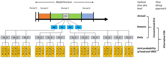
Figure 2.
Nested tree diagram of the stylized time slice approaches applied in the TIMES-CO-BBE model. Level 1—Seasons: FA: Fall; SP: Spring; SU: Summer; WI: Winter. Level 2—Daily time slices: D: Day hours; N: Night hours; P: Peak hours. Level 3—Joint probability of load and intermittent power supply: H: high probability; M: intermediate probability; L: low probability. Reprinted/adapted with permission from Ref. [36]. Copyright 2022, IEA-ETSAP.
Few direct integration methods have been proposed to enhance the temporal representation of VRES integration in ESOMs [5]. In the present study, an alternative approach (V36) was used based on introducing a time slice level that approximates the joint probability distribution of the load and VRES generation [4]. Three VRES supply levels (high, intermediate, and low) were defined for each of the 12 load time slices, thereby representing VRES at 36 time slices [56] (Figure 2). Compared to other direct integration techniques, Poncelet et al. [55] found this approach to effectively reduce the approximation error of RLDC at high penetration of VRES in the system, with reasonable ease of implementation and manageable computational complexity. The main limitation of this method is that it alters the chronology of supply and demand, which limits the capacity of the ESOM to assess the impact of the short-term dynamics of VRES and the corresponding potential of flexibility options such as energy storage or demand side management [4]. This limitation was addressed by assessing these short–term dynamics via a dedicated power model.
2.2.2. Hydropower Scenarios
Currently, 23 hydropower reservoirs are operating in Colombia, with a total installed capacity and technical useful volume exceeding 10 GW and 17 TWh, respectively [48,57]. These reservoirs are connected to a complex hydrological system comprising 34 rivers and multiple reservoir cascades [58]. The Colombian transmission system operator (XM) classifies these reservoirs into five hydrological zones (Antioquia, Caribe, Centro, Oriente, and Valle) [33] (Figure 3 and Supplementary S3).
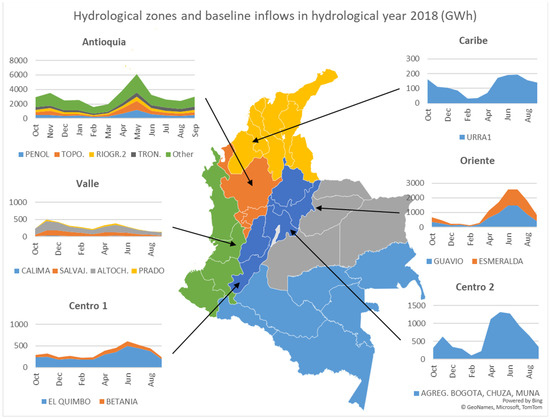
Figure 3.
Simplified representation of hydrological zones in Colombia and the corresponding monthly inflow patterns in GWh for the main reservoirs in the hydrological year 2018, as a representative of mean historical conditions.
Here, the impact of hydroclimatic variability on Colombia’s energy system was modeled in two steps. First, a baseline scenario was constructed based on an analysis of historical data. Second, future scenarios depicting hydroclimatic variability were formulated in relation to the baseline. For both steps, the corresponding patterns were parametrized and scaled to a spatio-temporal resolution that was suitable for each model.
For the baseline scenario, historical datasets were selected according to the following criteria: (a) hydropower data should be reported in energy terms per reservoir as opposed to per river because reporting per river would require a detailed hydrological analysis beyond the scope of this study, and (b) the dataset should be representative of historical mean conditions.
For criterion (a), the Colombian Electricity Information System (SIEL) database of UPME was used [59]. Datasets for relevant indicators were retrieved, namely, the inflows, generated electricity, and net effective capacity per reservoir, at a monthly resolution for the last five years.
For criterion (b) the national level monthly inflows during the last 20 years compared to the respective historical average, as reported by XM [60] was analyzed. Accordingly, the 2018 hydrological year (note that the hydrological year 2018 refers to the period between October 2017 and September 2018 [61]) was identified as a representative of historical mean conditions, and the 2016 hydrological year was a proxy for a strong El Niño drought event (Supplementary S3).
For the midcentury impact of hydroclimatic variability, two scenarios, based on GCMs of temperature and precipitation projections, namely, CESM1–BGC (a median projection for Colombia) and CNRM–CM5 (a dry projection), were considered (Figure 4). Arango–Aramburo et al. [15] used these scenarios to force a global hydrological model to generate run-off and estimated the net change in hydropower production compared to baseline conditions. While reference [15] considered two Representative Concentration Pathway (RCP) scenarios (4.5 and 8.5), here we only focused on the case where efforts are exerted to stabilize radiative forcing at 4.5 W/m2. This case is more in line with the high penetration of VRES in the energy system, and therefore, is more consistent with the aim of this study.
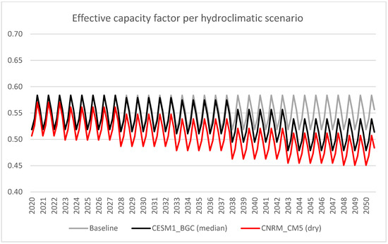
Figure 4.
Effective capacity factor of hydropower as represented in TIMES-CO-BBE, for the baseline conditions and median (CESM1_BGC) and dry (CNRM_CM5) hydroclimatic variability scenarios. For illustrative purposes, this figure represents a national level aggregation of eastern and western hydrological regions, as defined in this study.
For parametrization, the generation of hydropower in TIMES–CO–BBE was represented by static load factors, which determined the electricity generation as a fraction of the installed capacity. In contrast, PowerPlan takes the monthly inflows and the technical useful volumes of the reservoirs as inputs. Therefore, the storage and dispatch of hydropower can dynamically balance the supply and demand of electricity.
For the temporal resolution, TIMES–CO–BBE traces the generation of hydropower per season (quarterly) and conversely, PowerPlan simulates the inflows to the reservoirs in monthly time steps. For the spatial resolution, the inflows per reservoir in PowerPlan were spatially aggregated into six patterns that covered all five hydrological zones defined by XM. In TIMES–CO–BBE, these hydrological zones were grouped into a Western region (Antioquia, Centro, and Valle zones), and an Eastern region (Caribe and Oriente zones). The spatial aggregation of inflows/generation in a certain zone was implemented by summing the corresponding base year data of all reservoirs in this zone and calculating the respective normalized inflows/capacity factors for PowerPlan/TIMES–CO–BBE, respectively (Supplementary S3). It was assumed that future capacity expansion within a hydrological region would follow the same patterns as existing hydropower plants in that region.
Finally, future scenarios of hydroclimatic variability were retrieved in steps of five years and scaled down for TIMES–CO–BBE to seasonal time resolution and from a national to a regional level. A net loss of hydropower in a certain year was assumed to be equally distributed between the seasons and similarly, between the Eastern and Western regions (Figure 4).
2.3. Modeling Steps and Scenario Analysis
In this analysis the selected direct integration approach (Poncelet et al. [55]; de Wolf [56]) and the soft-linking approach (Lap et al. [31]) were combined through the following steps (Figure 5).
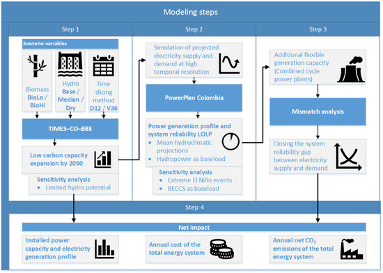
Figure 5.
Overview of the scenario analysis and modeling steps.
- Step 1: Long-term energy system optimization—the direct integration approach
Each scenario was initially implemented in the long-term planning energy system model to determine least cost pathways for the energy system at large. The scope of this analysis was on scenarios representing the SSP1 narrative, as described by Younis et al. [24], because they depict a socio–economic context that can enable steep learning curves of low carbon technologies and a rapid transition towards a low carbon economy.
The output of this step comprised the projected capacity expansion per type of power technology and the corresponding electricity generation mix. Moreover, the cost and emissions of the energy system were relevant inputs for Step 4. The focus was on the end of the time horizon, that is, mid–century projections, as an input to the power system model.
The main scenario variables considered were biomass availability and hydroclimatic variability. These were represented by two biomass cases (high and low potential) and three hydroclimatic scenarios (baseline, median, and dry). To apply the direct integration method, the combinations of these scenario variables were processed using the conventional D12 and the alternative V36 time slicing approaches. Consequently, 12 main scenarios were generated by TIMES–CO–BBE model. For a sensitivity analysis, another set of scenarios was investigated considering a limited expansion potential of hydropower.
- Step 2: Mid-century power system simulation—the soft-linking approach
The capacity expansion profiles obtained from the previous step were simulated in PowerPlan Colombia to analyze the dynamic dispatch at a high spatio–temporal resolution. The normalized hourly load factor was scaled to the installed capacity obtained by Step 1. The base year normalized hourly electricity demand was upscaled to the projected annual demand by 2050, assuming no interannual change in the pattern shape.
Each input scenario to PowerPlan was primarily simulated considering a dispatch order with hydropower as a base load, and biomass as a base load was briefly considered in a sensitivity analysis. Notably, the hydroclimatic scenarios from Step 1 depicted long-term alterations in mean-state rainfall induced by climate change. In PowerPlan, additional scenarios were simulated to evaluate the robustness of the capacity profiles from Step 1 in response to extreme El Niño drought anomalies. On a national level, the annual inflows of the simulated ENSO episode were approximately 30% less than the corresponding reference mean-state patterns.
The main outputs of this step included the electricity generation mix and the system reliability, quantified by the loss of load probability (LOLP). The LOLP was calculated at each hour by subtracting the total electricity generation of all power plants from the corresponding demand, where negative values indicated a loss of load. These values were summed up to the annual level.
- Step 3: Mismatch analysis—aligning power system reliability
In this step, the mismatch in system reliability for the scenarios simulated in Step 2 were addressed, particularly the main scenarios with hydropower as a base load, and the corresponding capacity-mixes subject to El Niño anomalies.
The mismatch analysis was conducted by aligning the LOLP of the scenarios simulated in Step 2 to a unified reliability target, which was set at ≤3 days per 10 years as a common range for present day industrialized economies. When the LOLP was >3, the power system was perceived as not being sufficiently reliable. The alignment was performed by introducing additional flexible power generation capacity of natural gas combined cycle power plants to fill the reliability gap. The additional capacity was iteratively simulated in steps of 250 MW, until the LOLP target was reached.
- Step 4: Technical, economic, and environmental impact
In this step, the results of the mismatch analysis were compared in relation to technical, economic, and environmental indicators. The main technical indicators included the capacity and electricity generation profiles and the additional flexible generation requirement.
The economic impact was quantified based on the total annual cost of the energy system by 2050, projected by TIMES–CO–BBE, and any additional costs incurred by additional capacity in PowerPlan Colombia. These costs included annualized capital expenditure (CAPEX), operational expenditure (OPEX), and the cost of fuel.
Similarly, the environmental impact was quantified by the CO2 emissions of the energy system and net changes incurred by the power simulation model for the mismatch analysis. For the scope of this analysis, the CO2 emissions were calculated based on Tier 2 emission factors of fuel combustion, following the guidelines of the Intergovernmental Panel on Climate Change (IPPC) [62].
3. Results
3.1. Least-Cost Capacity Expansion—The Direct Integration Approach
Figure 6 presents the mid-century projections of installed capacity and generated electricity, subject to low and high cases of biomass availability and baseline, median, and dry hydroclimatic scenarios. These least-cost projections are derived by the TIMES-CO-BBE model, using a standard (D12) and an alternative VRES time slice approach (V36).
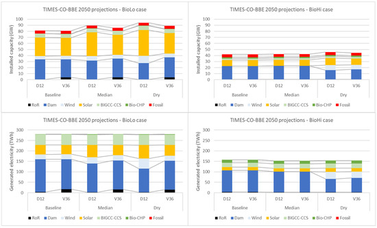
Figure 6.
Installed power capacity (upper row) and generated electricity (lower row) by 2050 in the TIMES-CO-BBE model for the low (left) and high (right) cases of biomass availability. Each case is projected considering baseline, median, and dry scenarios of hydroclimatic variability. A distinction is made between the use of conventional D12 and alternative V36 time slicing methods. These scenarios consider a reference technical potential of hydropower (>44 GW including existing capacity).
The influence of biomass availability is significant, as the power capacity and generation in BioLo is likely to be double compared to the BioHi case. This difference is driven by the endogenous demand for electrification in the TIMES–CO–BBE model. In a scenario with abundance of bioresources (BioHi), biofuels are expected to be the most cost-efficient solution to decarbonize the industrial heat and transport sectors. Should feedstock be constrained (BioLo), stringent GHG mitigation can still be achieved by the increased deployment of low-carbon electricity [24].
Notably the supply potential of biomass resources will likely depend on the capacity of the land-use sector to curb deforestation, upscale sustainable intensification practices in agriculture and agroforestry, and deliver sustainable bioenergy crops with net negative emissions [39,63].
Considering the variability of precipitation patterns, the capacity of hydropower is projected to expand in all scenarios and remain a major source of electricity. However, the predominance of hydro in the power mix is expected to decrease, especially in severely dry trajectories.
In the BioHi case, the retraction of hydropower can be modest because of the low demand for electricity. The role of fossil power can be overtaken by solar power as a low cost option and BECCS as a firm source of electricity and negative emissions. Moreover, the large-scale production of synthetic biofuels in these scenarios can raise the capacity of biorefineries to inject surplus electricity into the grid by up to 9% of the total electricity supply. In a dry trajectory, wind power can be a cost-competitive substitute for the expansion of hydropower, especially in the La Guajira region, where the highest wind speeds in mainland Colombia can be attained.
In the BioLo case, the capacity of hydropower can expand to 67–83% of the technical potential, and yet meet only 40–56% of the soaring demand for electrification. The deployment of scarce biomass resources in direct power production is likely to be more cost-efficient than biofuels, which can limit the role of biorefinery surpluses. A large-scale rollout of solar power is projected to make a cost-competitive contribution to the mix, while the role of wind power is likely to be more prominent under low precipitation than in baseline conditions. In a severely dry trajectory, up to 10–16% more power generation capacity than the corresponding baseline can be required to compensate for the climate-induced loss of hydropower and supply the same amount of electricity.
Regarding the temporal representation of VRES, the value of using the V36 direct integration method is tangible in scenarios where the conventional D12 time slicing projected a penetration of VRES above 30%. The difference is most pronounced in the dry scenarios, where the competitiveness of VRES against hydropower is likely to be higher than in the baseline scenarios.
In the most extreme scenarios (BioLo dry), the D12 predicted VRES to substitute the expansion of hydropower by up to 40% of electricity supply. In contrast, the V36 anticipated the climate-induced reduction of hydropower output to be partially alleviated by the increased expansion of hydropower capacity. Notably, the optimal solution is resolved at each time slice. Due to the smoothing effect of VRES patterns in the D12 method, it estimated VRES to meet 16% of the demand in the time slice with the highest peak. However, when the joint probability of the demand and the supply of VRES is articulated by the V36 method, the estimated contribution of VRES within the same peak time slice is reduced to 8%. This supply gap is projected to be compensated for by the expansion of run of river (ROR) and dam hydropower plants. More details on the capacity margin for VRES is reported in Supplementary S4.1.
Notably, the hydropower capacity in the scenarios mentioned above is projected to expand from the current level of approximately 12 GW to 16–37 GW (67–160 TWh). Such a magnitude lies within the technical potential of the Colombian hydropower atlas, and the exploitable potential estimated by Zhou et al. [64] (518 TWh). Based on the atlas, we considered a total potential (including existing power plants) of 40 GW and 4 GW, for large scale reservoirs and run of river, respectively [65]. These estimates exclude the potential in the Amazon region, because it is far from demand centers, infrastructure, and possibly has more ecological constraints than other regions [65]. In contrast, Arango–Aramburo et al. [15] assumed a significantly slowed rate of hydropower expansion.
Considering the sensitivity of the BioLo results in a limited potential for hydropower (<15 GW), a larger distinction is projected between D12 and V36 (Figure 7). Both methods expected wind power to increasingly replace the expansion of hydropower. Moreover, natural gas combined cycle power plants with CCS are anticipated to supply 2% and 5% of the demand in D12 and V36, respectively. While D12 predicted solar power to make a substantial contribution to the demand (22–24%), the V36 method downsized the feasible penetration of solar power to 13–15%, because of the enhanced temporal representation of VRES. Instead, the V36 opted for investment in more energy-efficient demand technologies to decrease the consumption of electricity, at a higher cost. These findings indicate that the tighter the constraints on affordable and flexible low carbon alternatives to VRES, which are hydropower and biomass in this case study, the higher the value of using the direct integration approach.
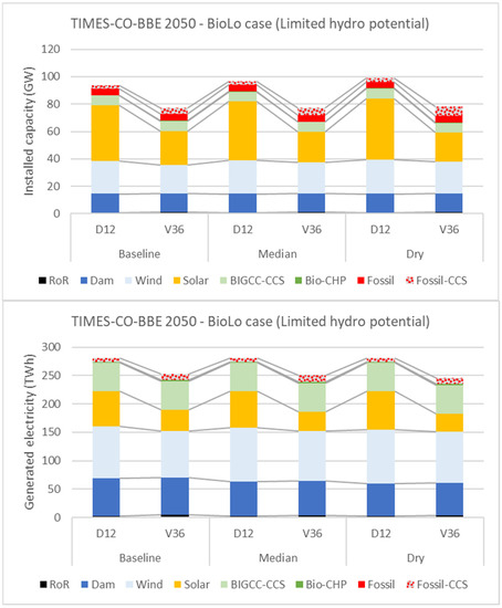
Figure 7.
Installed power capacity (upper row) and generated electricity (lower row) by 2050 in the TIMES-CO-BBE model for the low case of biomass availability, considering scenarios of hydroclimatic variability and alternative time slicing methods. These scenarios represent a sensitivity case where the expansion potential of hydropower is constrained (technical potential <15 GW including existing capacity).
3.2. Mismatch of System Reliability—The Soft–Linking Approach
Figure 8 displays the projected power generation capacity and electricity supply profiles by TIMES–CO–BBE (D12 and V36) and the corresponding simulations by PowerPlan Colombia for the reference hydro inflows and the case of an extreme El Niño drought event. The focus is on the dry hydroclimatic scenario where the model differences are most visible.
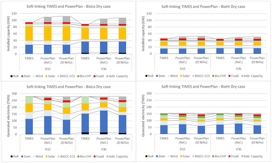
Figure 8.
Installed capacity (upper row) and generated electricity (lower row) by 2050 for low and high biomass supply potential cases (left and right, respectively) with a focus on the dry hydroclimatic scenario. These scenarios are projected by TIMES–CO–BBE by using D12 and V36 time slicing methods (direct integration approach). Via soft–linking and mismatch analysis, each scenario is simulated by the PowerPlan Colombia model and adjusted towards unified system reliability target. These simulations are performed for the reference dry climate patterns and a sensitivity case representing the impact of an extreme El Niño drought event on hydropower inflows.
TIMES–CO–BBE projected 100% renewable electricity from solar, wind, hydro, and biomass. This represents pathways to the Paris agreement where fossil powered assets would be eliminated, as discussed by Binsted et al. [66]. However, the soft–linking approach exposed the inadequacy of the modeled electricity mix to meet the demand.
The roles of hydropower and BECCS are expected to be more flexible in PowerPlan than in TIMES because of the dynamic dispatch and explicit representation of energy storage management in PowerPlan at a higher temporal resolution. When considering a dispatch order of hydropower dams as base load (Figure 8), the corresponding production of hydropower in PowerPlan Colombia is projected to be higher than in TIMES–CO–BBE, and that of BECCS is anticipated to be lower. In a sensitivity scenario with a dispatch of BECCS as the base load, the output of hydropower and BECCS in PowerPlan Colombia is projected to be similar to that in TIMES–CO–BBE (Supplementary S4.2). In both cases, the combined output of hydropower and BECCS in PowerPlan is anticipated to be comparable to that in TIMES.
The mismatch between supply and demand in PowerPlan Colombia can be partly alleviated by use of existing fossil-fueled capacity. However, this is insufficient to guarantee a reliable power supply. Based on the simulation of the BioLo dry capacity mix projected by TIMES–CO–BBE (D12), the LOLP is estimated at 980 days/10 years (Table 2). The corresponding LOLP using the V36 method is predicted to be lower (793 days/10 years) because of the lower penetration of VRES in this scenario.
Table 2.
Peak load, reserve factors, system reliability indicators, additional flexible generation capacity, system cost, and emissions for the dry hydroclimatic scenarios. The definition of key units is presented in the footnotes of the table.
To align the power supply in these scenarios to an adequate level of system reliability (LOLP ≤3 days per 10 years) using flexible natural gas combined cycle power plants, an additional capacity of 16 GW will be required to close this gap (Figure 8 and Table 2), which corresponds to 17–18% of the total power capacity projected by TIMES–CO–BBE. Accordingly, the grid penetration of VRES in D12, which is estimated by TIMES–CO–BBE at 40%, will be effectively reduced to 32%, and that in V36 will be effectively reduced from 27% to 21%. The corresponding supply of renewable electricity will be effectively reduced from 100% to 90% and 92% in D12 and V36, respectively.
Figure 9 shows the hourly simulation of the power mix from a sample week with high mismatch between demand and supply. The yellow areas in the figure show the use of flexible capacity to close this gap during peak load hours. While an excess supply of solar power is occasionally expected, the level of curtailment is projected to be much lower than peak load shortages. Under this system configuration, flexible generation is anticipated to play an important role that otherwise cannot be perfectly substituted with energy storage.
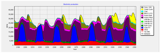
Figure 9.
A sample from the hourly simulation of power generation per technology in V36 BioLo Dry scenario (week 14). Yellow areas show the use of flexible capacity to close the gap between supply and demand during peak hours. The red line in day two shows an excess of solar power production.
The projected supply of solar and wind power by TIMES–CO–BBE is overestimated by 41% and 10%, respectively, relative to PowerPlan Colombia. The deviation in solar power can be mainly explained by factors considered in PowerPlan regarding the degeneration of the efficiency of solar panels, at 1% per year, as well as unplanned outage. These assumptions aim at improving the realism of the model. Supplementary S4.3 shows that overriding these assumptions can reduce the solar power generation gap between TIMES and PowerPlan models to 10%. Under such conditions, the contribution of fossil power could be reduced from 8–10% to 6%. The impact on the on the additional capacity requirement is estimated to be marginal.
Apart from climate-induced long-term alterations in mean-state rainfall, the robustness of the power system in response to extreme El Niño drought anomalies was also simulated (Figure 8 and Table 2). While the inflows of the simulated ENSO episode are 30% less than the reference mean-state patterns, the corresponding output of large-scale hydropower is anticipated to only be reduced by 18–20% because of the capacity of storage reservoirs in PowerPlan to regulate the inflows. To accommodate the El Niño effect, the dispatch of BECCS is projected to increase by 38% in D12 and higher (69%) in V36 because of the larger role of hydropower in V36 and consequently, its higher vulnerability to ENSO anomalies.
Despite the increased dispatch of BECCS, the capacity mix determined considering reference mean-state inflow patterns (Figure 8, middle bars) will possibly be insufficient to guarantee a reliable power supply during extreme El Niño drought anomalies. For an ENSO-proof system operation, the additional flexible capacity is anticipated to be 14–18% higher than the corresponding reference case, and the respective load factor of the additional capacity is expected to more than double. Under such conditions, the projected contribution of renewable electricity is further reduced to 85% of the total supply (Figure 8, right bars).
In the case of BioHi, similar trends are projected. However, their scale is expected to be smaller because of the relatively low demand for electricity and the higher contribution of biorefinery surpluses and existing fossil power plants to the mix. The corresponding additional capacity requirement is estimated at 6.0 GW (13%) and 5.3 GW (12%) in D12 and V36, respectively. The 100% supply of renewable electricity will be reduced to 91% and 92% in D12 and V36, respectively. Nevertheless, in the event of El Niño drought, the effective contribution of renewable power supply to a reliable system can be further reduced to 87%.
3.3. Implications for the Cost of the Energy System
Figure 10 and Table 2 demonstrate the total annual cost of the energy system as projected by TIMES–CO–BBE and the additional cost identified by PowerPlan Colombia as necessary to guarantee a reliable power system.
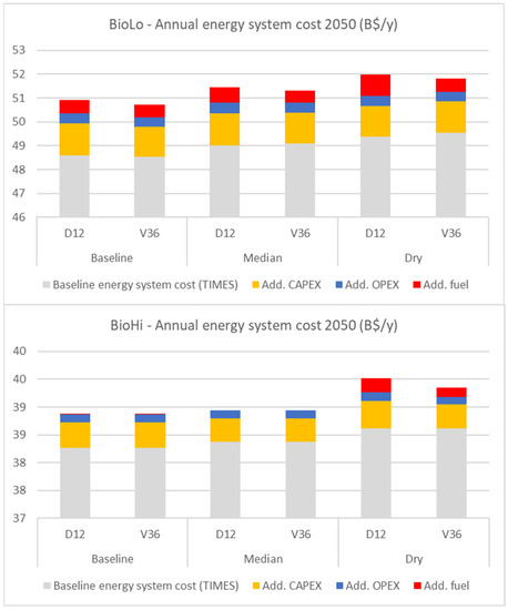
Figure 10.
Annual energy system cost for midcentury scenarios in B$/y (note the scale), including the total energy system cost estimated by the TIMES–CO–BBE model and the additional cost to guarantee a reliable power supply, calculated based on the PowerPlan Colombia model. Additional cost includes capital and operational cost of flexible power generation capacity, as well as cost of fuel for the additional capacity, existing fossil fuel power plants, and net change in biomass consumption.
The baseline system cost determined by TIMES–CO–BBE in the BioLo case is estimated to be higher by 27–28% (10–11 B$/y) than the corresponding scenarios in the BioHi case. This difference can be largely explained by the higher investment in powertrains for electric vehicles (at the expense of internal combustion engines running on synthetic biofuels), the cost of import of base chemicals (as opposed to domestic production of bio–based alternatives), and other costs in the energy conversion supply chain [24].
Regarding the impact of hydroclimatic variability, the energy system cost in a severely dry climate is likely to be 2% higher than that in the baseline hydroclimatic conditions in the BioLo case. This additional cost can be less in the BioHi case (1%) because of the lower reliance on hydropower and lower electricity demand.
When considering the implications for securing a reliable power system, the associated cost in the BioLo dry case is estimated to be 2.6 and 2.3 B$/y using D12 and V36 methods, respectively (Figure 10 and Table 2). That is, the projected energy system cost by TIMES–CO–BBE (D12) is underestimated by 5%, whereas the alternative V36 method can marginally reduce this gap to 4%. Logically, such a gap is expected to be less in the BioHi case (<1 B$/y or 2%) because of the lower requirement for reliability measures.
When examining the cost structure of these measures, the highest cost is expected to be the annualized CAPEX of flexible power generation capacity, followed by the cost of fuel. Notably, the reduced use of BECCS power plants as projected by PowerPlan Colombia can result in fuel savings compared to TIMES–CO–BBE. In some BioHi scenarios, the net savings in biomass consumption can be high enough to negate the cost of fossil fuels required to run the flexible generation capacity.
3.4. Implications for the Emissions of the Energy System
Figure 11 illustrates the mid-century CO2 balance of the energy system by 2050 as determined by TIMES–CO–BBE vis-à-vis the outcome of the mismatch analysis.
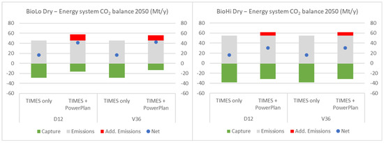
Figure 11.
Annual CO2 balance of the total energy system by 2050 as determined by TIMES–CO–BBE and net change incurred by additional measures to guarantee a reliable power system operation, as projected by PowerPlan Colombia.
An emissions target of 17 Mt/y by 2050 is set in TIMES–CO–BBE as an extrapolation of the Colombian NDC for 2030, inspired by projected RCP trends for Latin America [67]. This target corresponds to 85% emissions reduction with respect to the baseline emissions projected by TIMES–CO–BBE for the same year in the absence of an emissions mitigation policy. In contrast, the corresponding emissions in 2015 were estimated at approximately 88 Mt [68].
In BioLo dry, limited biomass resources are expected to be concentrated in BECCS power plants, capturing up to 29 Mt CO2 per year. Conversely, in BioHi dry, the deployment of BECCS technologies is anticipated to include both power and advanced gasification biofuels. The corresponding CO2 capture can reach 38 Mt/y, which can allow more positive emissions elsewhere in the energy system (the industry and built environment) [24].
Nevertheless, the mismatch analysis revealed that the emissions reduction pathway of 85% by 2050 in TIMES–CO–BBE will be effectively reduced to 62% and 72% in the BioLo and BioHi cases, respectively, should the power system reliability standard be considered. This disparity is because the soft-linking approach anticipated an increased use of fossil power plants, resulting in more positive emissions, and a decreased use of BECCS power plants, resulting in less negative emissions.
The increase in emissions is projected to be higher in BioLo than in BioHi because of the lower use of fossil capacity in BioHi. Moreover, much of the CO2 capture through BECCS in BioHi is expected to be from liquid biofuel production, which is less sensitive to the balancing of the power grid. The net emissions balance would be lower if BECCS power plants are dispatched as a base load, however, this would reflect on the increased consumption of biomass resources and incur higher energy system cost.
4. Discussion and Conclusions
The energy mixes projected by the modeling framework resemble those depicted in other mid-century decarbonization studies of the Colombian energy systems, such as Delgado et al. [18] using the GCAM model and Arango–Aramburo et al. [15] using a multi–model comparison, particularly their TIAM–ECN model, which has a similar architecture to TIMES–CO–BBE. The main overlaps include the declining role of hydropower, a substantial penetration of VRES, and the contribution of BECCS (and fossil CCS in scenarios with limited expansion potential for hydropower). Like Delgado et al. [18], the results presented here emphasized the relevance of sustainable agricultural intensification for biomass production, the importance of electrification and advanced biofuels in decarbonizing the transport sector, and the potential of the power sector as a net sink of CO2.
In contrast to Younis et al. [24] and the abovementioned studies, the challenges to the short-term operational flexibility of the power system were scrutinized. For the near future (2030), IRENA [30] and Pupo–Roncallo et al. [29] anticipated these challenges to be mild, even during El Niño droughts. However, the results of the present study suggest that these challenges are likely to be severe in the longer-term (given a deep decarbonization pathway), limiting the feasible penetration of VRES to 32%. Dealing with them can incur an additional overhead of 12–17% investment in flexible generation capacity, 2–5% of the annual energy system cost, and a 15–27% shortfall in achieving the aspired GHG mitigation target, with possible trade-offs between reducing cost and emissions. These figures are likely to be exacerbated in the event of extreme El Niño anomalies.
The estimates of the mismatch capacity are higher than the range projected by Lap et al. [31] for Brazil (11–17% of the total capacity requirement, as opposed to 3–14%). The difference can possibly be explained by the lower penetration of solar PV and wind power in the Brazilian case (<25% of electricity supply, mostly wind). In contrast, Lap et al. [31] projected a large role for concentrated solar power with thermal energy storage as a relatively steady source of low carbon power. Another explanation, which highlights a limitation in the present analysis, is the absence of demand response measures from the scope of this analysis, particularly in scenarios with a large rollout of battery electric vehicles. When comparing alternative charging behaviors, Lap et al. [31] found that smart charging could considerably decrease the need for additional capacity requirement by shifting the charging time to off-peak hours. Note that the power mixes projected by TIMES-CO-BBE corresponded to large expansion of low carbon flexible generation capacities, namely from hydropower reservoir and BIGCC-CCS, where the reserve factor ranged between 2.2–2.7 (see Table 2). Under such conditions, the curtailment of VRES power was too low to consider energy storage as a balancing option in PowerPlan (below 300 GWh per year). Future research can consider modeling more balancing options, for example, pumped hydro storage [69], and demand side management.
In relation to the impact of climate change, the scope of the present study was limited to hydropower because of its critical role in the case of Colombia. Therefore, the potential impact on the supply of other renewable energy sources and the demand for cooling and heating were neglected. Conclusions about these impacts have been mixed and uncertain across regions [70]. Relevant impacts to Colombia include the likelihood of increased demand for cooling in Latin America [70] and a modest change in the solar energy potential in most tropical areas [71]. Quantifying the climate impacts on bioenergy potential remains complex because of its overlap with uncertain factors such as future land and water availability [70]. Here, it is argued that the uncertainty of biomass supply potential has been sufficiently covered in the present analysis by considering a wide range of land availability for biomass.
When reflecting on the modeling framework, the direct integration method (V36 versus D12) could consistently reduce the ESOM’s overestimation of the feasible penetration of VRES and the underestimation of the system cost. This was verified by simulating different scenarios at an hourly resolution. Despite the marginal difference in the system cost between D12 and V36, it can translate into several billions of US dollars in annual savings. As highlighted by Poncelet et al. [55], the limited capacity of this method to address the short-term operation and flexibility requirement of the power system is recognized. In this regard, combining this method with soft-linking has been shown to be complementary and outperformed the use of either of the two methods individually.
In conclusion, this study presented a combined approach for two state-of-the-art methods that capture the techno-economic challenges of the large-scale integration of intermittent renewable energy sources in long-term planning energy system optimization models. This approach was used to analyze trajectories towards the deep decarbonization of the Colombian energy system by mid-century, subject to future uncertainty of hydroclimatic conditions and the development of the bioeconomy.
The direct integration method, based on approximating the joint probability distribution of load and supply from intermittent renewable energy sources, could capture the limitation of these sources at a grid penetration >30%, especially under the high limitation of alternative flexible low carbon energy sources. However, the loss of chronology in this method inhibits it from assessing the value of flexibility options and the reliable operation of the power system in the short-term.
This limitation can be effectively addressed by soft-linking the improved energy system model with a power system simulation model. The power system simulation model can quantify the need for flexibility options and their implications for the cost and emissions of the energy system. Combining both methods can yield closer results to the global optimum solution than either of them individually, as confirmed by simulation at an hourly resolution.
Supplementary Materials
The following supporting information can be downloaded at: https://www.mdpi.com/article/10.3390/en15207604/s1.
Author Contributions
Conceptualization, A.Y., R.B. and A.F.; data curation, A.Y., R.B., J.R. and M.d.W.; formal analysis, A.Y., R.B. and J.R.; funding acquisition, A.F.; investigation, R.B.; methodology, A.Y., R.B., J.R. and M.d.W.; project administration, A.Y.; resources, A.F.; software, R.B.; supervision, R.B. and A.F.; validation, A.Y., R.B., M.d.W. and A.F.; visualization, A.Y.; writing–original draft, A.Y.; writing–review & editing, A.Y. All authors have read and agreed to the published version of the manuscript.
Funding
This research and the APC were funded by Netherlands Enterprise Agency (RVO) grant number TF13COPP7B.
Data Availability Statement
The data presented in this study are available in the manuscript and the Supplementary Materials any additional data can be requested from the corresponding author.
Acknowledgments
Special thanks to Tjerk Lap for his suggestions to improve this work. Thanks to the International Energy Agency–Energy Technology Systems Analysis Programme (IEA-ETSAP) for granting us the permission to use and modify Figure 2.1 from the manual of the TIMES model, as presented in Figure 2 in this manuscript.
Conflicts of Interest
The authors declare no conflict of interest.
Abbreviations
| BECCS | Bioenergy combined with carbon capture and storage |
| CCS | Carbon capture and storage |
| CGE | Computational general equilibrium |
| ENSO | El Niño and la Niña Southern Oscillation |
| ESOM | Energy system optimization model |
| GCAM | Global change analysis model |
| GCM | Global circulation model |
| GHG | Greenhouse gas |
| IAM | Integrated assessment model |
| LDC | Load duration curve |
| LOLP | Loss of load probability |
| NDC | Nationally determined contribution |
| RCP | Representative Concentration Pathway |
| RLDC | Residual load duration curve |
| SIEL | The Colombian Electricity Information System database |
| UPME | Colombian Energy and Mining Planning Office |
| VRES | Variable renewable energy sources |
| XM | The Colombian transmission system operator |
| RCP | Representative Concentration Pathway |
References
- Edenhofer, O.; Pichs-Madruga, R.; Sokona, Y.; Kadner, S.; Minx, J.C.; Brunner, S.; Agrawala, S.; Baiocchi, G.; Bashamakov, I.A.; Blanco, G.; et al. Technical Summary. In Climate Change 2014: Mitigation of Climate Change. Contribution of Working Group III to the Fifth Assessment Report of the Intergovernmental Panel on Climate Change; Edenhofer, O., Pichs-Madruga, R., Sokona, Y., Farahani, E., Kadner, S., Seyboth, K., Adler, A., Baum, I., Brunner, S., Eds.; Cambridge University Press: Cambridge, UK; New York, NY, USA, 2014; pp. 527–532. [Google Scholar] [CrossRef]
- Luderer, G.; Krey, V.; Calvin, K.; Merrick, J.; Mima, S.; Pietzcker, R.; Van Vliet, J.; Wada, K. The role of renewable energy in climate stabilization: Results from the EMF27 scenarios. Clim. Change 2013, 123, 427–441. [Google Scholar] [CrossRef]
- Brouwer, A.S.; van den Broek, M.; Seebregts, A.; Faaij, A. Impacts of large-scale Intermittent Renewable Energy Sources on electricity systems, and how these can be modeled. Renew. Sustain. Energy Rev. 2014, 33, 443–466. [Google Scholar] [CrossRef]
- Collins, S.; Deane, J.P.; Poncelet, K.; Panos, E.; Pietzcker, R.C.; Delarue, E.; Gallachóir, B.P.Ó. Integrating short term variations of the power system into integrated energy system models: A methodological review. Renew. Sustain. Energy Rev. 2017, 76, 839–856. [Google Scholar] [CrossRef]
- Das, P.; Mathur, J.; Bhakar, R.; Kanudia, A. Implications of short-term renewable energy resource intermittency in long-term power system planning. Energy Strategy Rev. 2018, 22, 1–15. [Google Scholar] [CrossRef]
- Ang, B.; Su, B. Carbon emission intensity in electricity production: A global analysis. Energy Policy 2016, 94, 56–63. [Google Scholar] [CrossRef]
- XM. Capacidad Efectiva Neta. Reporte Integral de Sostenibilidad, Operación y Mercado 2020. Available online: https://informeanual.xm.com.co/2020/informe/pages/xm/24-capacidad-efectiva-neta.html (accessed on 31 March 2021).
- van Vliet, M.; van Beek, L.; Eisner, S.; Flörke, M.; Wada, Y.; Bierkens, M.F. Multi-model assessment of global hydropower and cooling water discharge potential under climate change. Glob. Environ. Change 2016, 40, 156–170. [Google Scholar] [CrossRef]
- Poveda, G.; Álvarez, D.M.; Rueda, Ó.A. Hydro-climatic variability over the Andes of Colombia associated with ENSO: A review of climatic processes and their impact on one of the Earth’s most important biodiversity hotspots. Clim. Dyn. 2010, 36, 2233–2249. [Google Scholar] [CrossRef]
- Duque, J.P.B.; García, J.J.; Velásquez, H. Efectos del cargo por confiabilidad sobre el precio spot de la energía eléctrica en Colombia. Cuad. Econ. 2016, 35, 491–519. [Google Scholar] [CrossRef]
- XM. Huella del Carbono. En Mov Boletín XM Para Los Agentes Del Sect Eléctrico Edición 09–Julio 2016. Available online: https://www.xm.com.co/EnMovimiento/Pages/default-Jul2016.aspx (accessed on 1 April 2021).
- Turner, S.W.; Ng, J.Y.; Galelli, S. Examining global electricity supply vulnerability to climate change using a high-fidelity hydropower dam model. Sci. Total Environ. 2017, 590–591, 663–675. [Google Scholar] [CrossRef]
- Steinhoff, D.F.; Monaghan, A.; Clark, M.P. Projected impact of twenty-first century ENSO changes on rainfall over Central America and northwest South America from CMIP5 AOGCMs. Clim. Dyn. 2014, 44, 1329–1349. [Google Scholar] [CrossRef]
- Turner, S.W.; Hejazi, M.; Kim, S.H.; Clarke, L.; Edmonds, J. Climate impacts on hydropower and consequences for global electricity supply investment needs. Energy 2017, 141, 2081–2090. [Google Scholar] [CrossRef]
- Arango-Aramburo, S.; Turner, S.W.; Daenzer, K.; Ríos-Ocampo, J.; Hejazi, M.I.; Kober, T.; Álvarez-Espinosa, A.C.; Romero-Otalora, G.D.; van der Zwaan, B. Climate impacts on hydropower in Colombia: A multi-model assessment of power sector adaptation pathways. Energy Policy 2019, 128, 179–188. [Google Scholar] [CrossRef]
- Candil, N.A.N.; Moreno, J.R.; Castañeda, J.F.F.; Villazón, R.A.; Galvis, J.J.M. La Cadena del Carbón; Unidad de Planeación Minero Energética: Bogotá, Colombia, 2012. [Google Scholar]
- Calderón, S.; Alvarez, A.C.; Loboguerrero, A.M.; Arango, S.; Calvin, K.; Kober, T.; Daenzer, K.; Fisher-Vanden, K. Achieving CO2 reductions in Colombia: Effects of carbon taxes and abatement targets. Energy Econ. 2016, 56, 575–586. [Google Scholar] [CrossRef]
- Delgado, R.; Wild, T.B.; Arguello, R.; Clarke, L.; Romero, G. Options for Colombia’s mid-century deep decarbonization strategy. Energy Strategy Rev. 2020, 32, 100525. [Google Scholar] [CrossRef]
- Gobierno de Colombia. Actualización de la Contribución Determinada a Nivel Nacional de Colombia (NDC); Gobierno de Colombia: Bogotá, Colombia, 2020.
- UPME. Integración de las Energías Renovables no Convencionales en Colombia: Resumen Ejecutivo; UPME: Bogotá, Colombia, 2015; ISSN 0121-4993. [Google Scholar]
- Wicke, B.; Van Der Hilst, F.; Daioglou, V.; Banse, M.; Beringer, T.; Gerssen-Gondelach, S.; Heijnen, S.; Karssenberg, D.; Laborde, D.; Lippe, M.; et al. Model collaboration for the improved assessment of biomass supply, demand, and impacts. GCB Bioenergy 2014, 7, 422–437. [Google Scholar] [CrossRef]
- Gerssen-Gondelach, S.; Saygin, D.; Wicke, B.; Patel, M.; Faaij, A. Competing uses of biomass: Assessment and comparison of the performance of bio-based heat, power, fuels and materials. Renew. Sustain. Energy Rev. 2014, 40, 964–998. [Google Scholar] [CrossRef]
- Johansson, V.; Lehtveer, M.; Göransson, L. Biomass in the electricity system: A complement to variable renewables or a source of negative emissions? Energy 2018, 168, 532–541. [Google Scholar] [CrossRef]
- Younis, A.; Benders, R.; Delgado, R.; Lap, T.; Gonzalez-Salazar, M.; Cadena, A.; Faaij, A. System analysis of the bio-based economy in Colombia: A bottom-up energy system model and scenario analysis. Biofuels Bioprod. Biorefining 2020, 15, 481–501. [Google Scholar] [CrossRef]
- Bahn, O.; Cadena, A.; Kypreos, S. Joint implementation of CO2 emission reduction measures between Switzerland and Colombia. Int. J. Environ. Pollut. 1999, 12, 308–322. [Google Scholar] [CrossRef]
- Delgado, R.; Álvarez, C.; Cadena, Á.; Calderón, S. Modelling the Socio Economic Implications of Mitigation Actions in Colombia: Working Paper for the CDKN Project on LINKING Sectoral and Economy Wide Models; CKDN: Quito, Ecuador, 2014. [Google Scholar]
- Pfenninger, S.; Hawkes, A.; Keirstead, J. Energy systems modeling for twenty-first century energy challenges. Renew. Sustain. Energy Rev. 2014, 33, 74–86. [Google Scholar] [CrossRef]
- Després, J.; Hadjsaid, N.; Criqui, P.; Noirot, I. Modelling the impacts of variable renewable sources on the power sector: Reconsidering the typology of energy modelling tools. Energy 2014, 80, 486–495. [Google Scholar] [CrossRef]
- Pupo-Roncallo, O.; Campillo, J.; Ingham, D.; Hughes, K.; Pourkashanian, M. Large scale integration of renewable energy sources (RES) in the future Colombian energy system. Energy 2019, 186, 115805. [Google Scholar] [CrossRef]
- IRENA. Colombia Power System Flexibility Assessment: IRENA Flextool Case Study; IRENA: Bonn, Germany, 2018. [Google Scholar]
- Lap, T.; Benders, R.; van der Hilst, F.; Faaij, A. How does the interplay between resource availability, intersectoral competition and reliability affect a low-carbon power generation mix in Brazil for 2050? Energy 2020, 195, 116948. [Google Scholar] [CrossRef]
- DecisionWare Group. TIMES-Starter Model Guidelines for Use, Version 1.0; DecisionWare Group: Paris, France, 2016. [Google Scholar]
- XM. Embalses. Hirdologuía 2021. Available online: https://www.xm.com.co/Paginas/Hidrologia/Embalses.aspx (accessed on 30 April 2021).
- Lap, T.; Benders, R.; Köberle, A.; van der Hilst, F.; Nogueira, L.; Szklo, A.; Schaeffer, R.; Faaij, A. Pathways for a Brazilian biobased economy: Towards optimal utilization of biomass. Biofuels Bioprod. Biorefining 2019, 13, 673–689. [Google Scholar] [CrossRef]
- de Vita, A.; Kielichowska, I.; Mandatowa, P.; Capros, P.; Dimopoulou, E.; Evangelopoulou, S. ASSET Project: Technology Pathways in Decarbonisation Scenarios; Tractebel, Ecofys, E3-Modelling: Brussels, Belgium, 2018. [Google Scholar]
- Loulou, R.; Remme, U.; Kanudia, A.; Lehtila, A.; Goldstein, G. Documentation for the TIMES Model Part I; IEA-ETSAP: Paris, France, 2005. [Google Scholar]
- O’Neill, B.C.; Kriegler, E.; Ebi, K.L.; Kemp-Benedict, E.; Riahi, K.; Rothman, D.S.; van Ruijven, B.J.; van Vuuren, D.P.; Birkmann, J.; Kok, K.; et al. The roads ahead: Narratives for shared socioeconomic pathways describing world futures in the 21st century. Glob. Environ. Change 2017, 42, 169–180. [Google Scholar] [CrossRef]
- Gobierno de Colombia. Colombia’s Intended Nationally Determined Contribution (INDC) [Unofficial English Translation]; Gobierno de Colombia: Bogotá, Colombia, 2015.
- Younis, A.; Trujillo, Y.; Benders, R.; Faaij, A. Regionalized cost supply potential of bioenergy crops and residues in Colombia: A hybrid statistical balance and land suitability allocation scenario analysis. Biomass Bioenergy 2021, 150, 106096. [Google Scholar] [CrossRef]
- de Vries, H.J.M.; Benders, D.R.M.J. Powerplan: An Interactive Simulation Tool to Explore Electric Power Planning Options. In Integrated Electricity Resource Planning; de Almeida, A.T., Rosenfeld, A.H., Roturier, J., Norgard, J., Eds.; Springer: Dordrecht, The Netherlands, 1994; pp. 123–135. [Google Scholar] [CrossRef]
- Benders, R.M.J. Interactive Simulation of Electricity Demand and Production; University of Groningen: Groningen, The Netherlands, 1996. [Google Scholar]
- Thiam, D.-R.; Benders, R.M.; Moll, H.C. Modeling the transition towards a sustainable energy production in developing nations. Appl. Energy 2012, 94, 98–108. [Google Scholar] [CrossRef]
- Urban, F.; Benders, R.M.J.; Moll, H. Renewable and low-carbon energies as mitigation options of climate change for China. Clim. Change 2009, 94, 169–188. [Google Scholar] [CrossRef]
- Younis, A. Exploring Long-term Strategies for Egypt’s Power System with a Scenario Modelling Approach; University of Groningen: Groningen, The Netherlands, 2015. [Google Scholar]
- Younis, A. Water and Electricity: Using Systems Analysis to Explore Potential International Conflicts and Resolutions Related to the Grand Ethiopian Renaissance Dam (GERD) Project; University of Groningen: Groningen, The Netherlands, 2015. [Google Scholar]
- van Meerwijk, A.J.H.; Benders, R.M.J.; Davila-Martinez, A.; Laugs, G.A.H. Swiss pumped hydro storage potential for Germany’s electricity system under high penetration of intermittent renewable energy. J. Mod. Power Syst. Clean Energy 2016, 4, 542–553. [Google Scholar] [CrossRef]
- Ramírez Cardoso, J.A. Low-Carbon Strategies for the Power System in COLOMBIA 2050; University of Groningen: Groningen, The Netherlands, 2018. [Google Scholar]
- XM. Capacidad Efectiva por Tipo de Generación. Parámetros Técnicos Del SIN 2021. Available online: http://paratec.xm.com.co/paratec/SitePages/generacion.aspx?q=capacidad (accessed on 30 April 2021).
- IDEAM. Atlas de Radiación Solar, Ultravioleta y Ozono de Colombia—Interactivo n.d. Available online: http://atlas.ideam.gov.co/visorAtlasRadiacion.html (accessed on 15 April 2019).
- IDEAM. Atlas de Viento de Colombia—Interactivo n.d. Available online: http://atlas.ideam.gov.co/visorAtlasVientos.html (accessed on 15 April 2019).
- Pfenninger, S.; Staffell, I. Long-term patterns of European PV output using 30 years of validated hourly reanalysis and satellite data. Energy 2016, 114, 1251–1265. [Google Scholar] [CrossRef]
- Staffell, I.; Pfenninger, S. Using bias-corrected reanalysis to simulate current and future wind power output. Energy 2016, 114, 1224–1239. [Google Scholar] [CrossRef]
- XM. Informe de Operación del SIN y Administración del Mercado 2015; XM: Medellín, Colombia, 2016. [Google Scholar]
- Ueckerdt, F.; Brecha, R.; Luderer, G.; Sullivan, P.; Schmid, E. Variable Renewable Energy in Modeling Climate Change Mitigation Scenarios, 4th ed.; Physics Faculty Publications: Dayton, OH, USA, 2011. [Google Scholar]
- Poncelet, K.; Delarue, E.; Six, D.; Duerinck, J.; D’Haeseleer, W. Impact of the level of temporal and operational detail in energy-system planning models. Appl. Energy 2016, 162, 631–643. [Google Scholar] [CrossRef]
- de Wolf, M. The Future Role of Power to Gas in The Netherlands: An Energy-System Wide Analysis; University of Groningen: Groningen, The Netherlands, 2021. [Google Scholar]
- XM. Volumen Embalses. Parámetros Técnicos Del SIN 2021. Available online: http://paratec.xm.com.co/paratec/SitePages/hidrologia.aspx?q=volumen (accessed on 30 April 2021).
- Macias, A.M.; Andrade, J. Estudio de Generación Bajo Escenarios de Cambio Climatico; XM: Bogotá, Colombia, 2014. [Google Scholar]
- UPME. Consultas Estadísticas de Generación. Sist Inf Eléctrico Colomb 2021. Available online: http://www.siel.gov.co/Inicio/Generación/Generación1/tabid/143/Default.aspx (accessed on 4 May 2021).
- XM. 21. Oferta y Generación/Aportes. Reporte Integral de Sostenibilidad, Operación y Mercado 2019. Available online: https://informeanual.xm.com.co/demo_3/pages/xm/21-aportes.html (accessed on 4 May 2021).
- Ng, J.Y.; Turner, S.W.D.; Galelli, S. Influence of El Niño Southern Oscillation on global hydropower production. Environ. Res. Lett. 2017, 12, 034010. [Google Scholar] [CrossRef]
- IPCC. Volume 2 Energy. In 2006 IPCC Guidelines for National Greenhouse Gas Inventories; Eggleston, S., Buendia, L., Miwa, K., Ngara, T., Tanabe, K., Eds.; IGES: Kanagawa, Japan, 2006; p. 29. [Google Scholar]
- Ramírez-Contreras, N.; Munar-Florez, D.; Hilst, F.; Espinosa, J.; Ocampo-Duran, Á.; Ruíz-Delgado, J.; Molina-López, D.; Wicke, B.; Garcia-Nunez, J.; Faaij, A. GHG Balance of Agricultural Intensification & Bioenergy Production in the Orinoquia Region, Colombia. Land 2021, 10, 289. [Google Scholar] [CrossRef]
- Zhou, Y.; Hejazi, M.; Smith, S.; Edmonds, J.; Li, H.; Clarke, L.; Calvin, K.; Thomson, A. A comprehensive view of global potential for hydro-generated electricity. Energy Environ. Sci. 2015, 8, 2622–2633. [Google Scholar] [CrossRef]
- UPME. Atlas Potencial Hidroenergético de Colombia; UPME: Bogotá, Colombia, 2015. [Google Scholar]
- Binsted, M.; Iyer, G.; Edmonds, J.; Vogt-Schilb, A.; Arguello, R.; Cadena, A.; Delgado, R.; Feijoo, F.; Lucena, A.F.P.; McJeon, H.; et al. Stranded asset implications of the Paris Agreement in Latin America and the Caribbean. Environ. Res. Lett. 2020, 15, 044026. [Google Scholar] [CrossRef]
- Rogelj, J.; Popp, A.; Calvin, K.V.; Luderer, G.; Emmerling, J.; Gernaat, D.; Fujimori, S.; Strefler, J.; Hasegawa, T.; Marangoni, G.; et al. Scenarios towards limiting global mean temperature increase below 1.5 °C. Nat. Clim. Change 2018, 8, 325–332. [Google Scholar] [CrossRef]
- Pulido, A.D.; Chaparro, N.; Granados, S.; Ortiz, E.; Rojas, A.; Torres, F.; Turriago, J.D. Informe de Inventario Nacional de GEI de Colombia; IDEAM: Bogotá, Colombia, 2019. [Google Scholar]
- Pupo-Roncallo, O.; Ingham, D.; Pourkashanian, M. Techno-economic benefits of grid-scale energy storage in future energy systems. Energy Rep. 2020, 6, 242–248. [Google Scholar] [CrossRef]
- Yalew, S.G.; van Vliet, M.T.; Gernaat, D.E.H.J.; Ludwig, F.; Miara, A.; Park, C.; Byers, E.; De Cian, E.; Piontek, F.; Iyer, G.; et al. Impacts of climate change on energy systems in global and regional scenarios. Nat. Energy 2020, 5, 794–802. [Google Scholar] [CrossRef]
- Gernaat, D.E.H.J.; de Boer, H.S.; Daioglou, V.; Yalew, S.G.; Müller, C.; van Vuuren, D.P. Climate change impacts on renewable energy supply. Nat. Clim. Change 2021, 11, 119–125. [Google Scholar] [CrossRef]


Publisher’s Note: MDPI stays neutral with regard to jurisdictional claims in published maps and institutional affiliations. |
© 2022 by the authors. Licensee MDPI, Basel, Switzerland. This article is an open access article distributed under the terms and conditions of the Creative Commons Attribution (CC BY) license (https://creativecommons.org/licenses/by/4.0/).