Abstract
The present paper gives an overview of modelling methods of standard grounding systems under surge conditions, using the non-uniform transmission line approach. The model presented considers the soil ionization and the frequency dependence of the soil parameters during the current transients. Furthermore, the representation of the non-linear response of the soil is made using a shunt time-variable resistance to simulate the behavior of the grounding resistance when a surge current flows through the system. The model development and analysis are made using ATP-EMTP/ATPDraw transient software.
1. Introduction
Grounding systems are fundamental parts of a power system’s protection [1,2,3,4,5]. Grounding impedance may decrease, avoiding the effects of overvoltages produced in the system [6]. In addition, the system must prevent the breakdown of the dielectric of the electrical devices. Finally, it must also protect people against electric shocks produced from static charges stored in the electrical equipment [7]. All these requirements must be met at the lowest possible cost.
The grounding system is composed of three components according [3], namely:
- the metallic conductor that drives the current to the electrode;
- the electrode that is buried in the soil;
- the ground around the electrode. (It may be mentioned that the analysis of the behavior of the soil is the most important.)
For the analysis of the behavior of different types of grounding system under surge currents, different parameters of the soil and current computer simulations can be considered [8,9,10,11,12,13,14,15].
The circuit model based on a distributed network of a non-uniform transmission lines is preferred for modelling grounding systems under surge currents due to its ability to simulate the shape of the ionized region of the ground as a set of cylindrical zones that will change in time. In addition, the representation of the non-linear response of the soil can be reproduced by a shunt time-variable resistance to simulate the behavior of the grounding resistance when a surge current flows through the system.
The circuit model can be implemented in a computer software dedicated to transient analysis. Such an approach is helpful for engineers to predict the impulse characteristics of a grounding system under surge conditions. The simulation results can be obtained, e.g., by ATPDraw. This software can be used for the design of a grounding system. The models implemented will be compared with the real results.
In the present paper the behavior of two grounded systems under surge currents are reported with the aim to illustrate methods of grounding systems simulations. The analysis will be made considering the influence of some parameters of the soil and the surge current and how they affect the impulse grounding response and the transient ground potential rise of the system.
The aim of this paper is to discuss a model of a standard grounding system using the ATPDraw tool to simulate the non-linear response of the grounding resistance around the electrode produced by a surge current. To obtain a correct design of a standard grounding system, a circuit model based on a distributed network of a non-uniform transmission line is used.
2. Materials and Method
There are two factors that change the behavior of the grounding resistance when an impulsive current is flowing in a grounding system. The first one is the dependence of the permittivity and resistivity of the soil on the frequency of the current. The ground parameters mentioned before decrease when the frequency of the current signal increases. The second factor is the ionization of the soil due to the high value of the amplitude of the impulsive current.
When an impulsive current flows through the electrode to ground, an electric field is produced by this current around the electrode in ground [16]. The magnitude of this electric field is calculated using the Equation (1) given by [17]:
where J is the current density and is the resistivity of one-layer homogeneous soil when the surge current is flowing through the earth.
When the high frequency current flowing to earth increases too much, it means that the current density will increase too. An electric arc in the earth is generated due to this high value of current density, which produces a big decrement of the soil resistivity [18]. When a surge current with high amplitude is applied to the electrode, a breakdown zone is produced in the ground around the electrode [19]. This zone is shown in Figure 1.
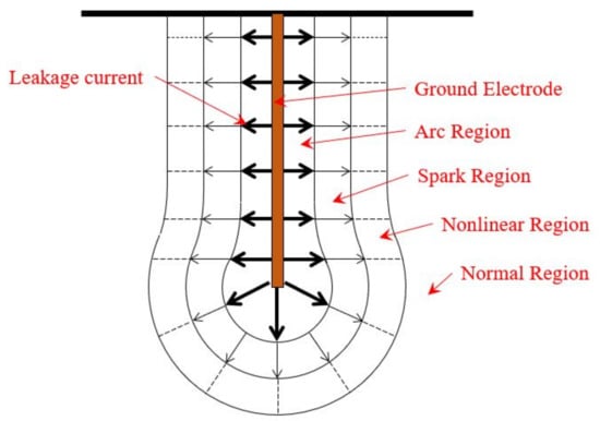
Figure 1.
Soil breakdown region in a grounding electrode.
The zones in the ground around the electrode that are known as the spark region, nonlinear region and normal region can be represented as the ionization zone, deionization zone and the non-ionization zone.
When the soil ionization phenomenon occurs, the soil resistivity value decreases because of the electric discharge produced around the electrode in the earth. However, when the process of deionization happens, the soil resistivity starts increasing again [20,21,22].
Soil ionization is the condition that makes the grounding resistance decrease in value when a high current is flowing from the electrode to earth [23]. The minimum value of the grounding resistance is at the peak of the surge current [24,25].
Soil ionization is generated when the electric field produced by the current exceeds the critical electric field of the soil [15]. However, it is important to mention the effects determining soil ionization because this depends on the current characteristics, ground electrode configuration, and soil characteristics and conditions [26,27].
Analysis of the soil critical electric field can determine the impulse behavior of the grounding system [28]. The critical electric field can be calculated using Equation (2), given by [29]:
where ρ is the resistivity of the soil and Ec is the critical electric field of the soil in [kV/m]. However, according to the IEEE group, the recommended critical electric field is 10 kV/cm [30].
The soil ionization produced around the conductor can be calculated using the circuit approach, where the grounding impedance decreases in value when a surge current is flowing through the grounding system [31,32,33,34,35]. This circuit method allows simulating the transient phenomena in the time domain.
Another method that is used for the analysis of the grounding system under lightning currents is the finite element method [36,37,38].
When the ground conditions are breaking down, the soil stops being dielectric and starts conducting; therefore, it can be assumed that the diameter of the electrode increases [39]. In this case, the leakage current will be not equal along the conductor because of the inductive effect produced by the high frequency of the surge current flowing in the electrode. The value of the higher leakage current is at the point where the surge current is applied [40]. Therefore, it is good to mention that the ionization zone around the electrode produced in the earth is not column-uniform [41], and it will generate a pyramidal region (Figure 2).
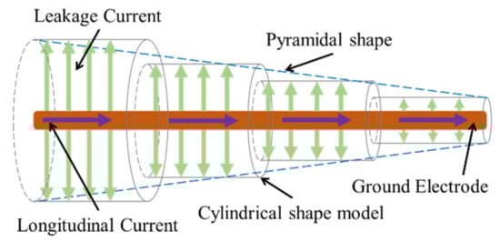
Figure 2.
Ionized zone of the soil around the electrode.
This pyramidal shape used to represent the ionized zone in the soil is a bit difficult to implement in the simulations. Therefore, a model of cylindrical shape to represent the ionized zone makes the simulations easier [42]. This model is shown in Figure 2.
For this cylindrical model, the electrode has a radius “a” and “ai” is the equivalent radius of the cylindrical zones [43]. The cylindrical zone with high equivalent radius will be situated at the beginning, where the surge current is injected, and the subsequent zones will decrease their equivalent radius [44].
The value of the equivalent radius of the cylindrical zones will be as big as the electric field produced by the leakage current after the soil ionization is produced. The equivalent radius will change according to the leakage current, which is time variable; therefore, this parameter will change over time [45].
The grounding electrode under surge currents can be characterized as a distributed network, because it can represent the ionized zone and the frequency dependent effects of the ground and electrodes [46]. Each cylindrical zone can be represented as a segment with a lumped parameters model as shown in the Figure 3 [47].
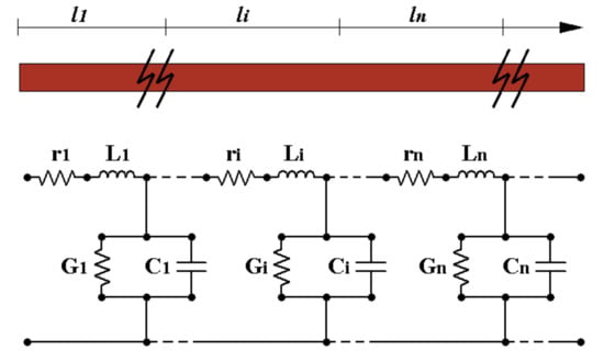
Figure 3.
Representation of a grounding electrode.
The length of the segment should be selected considering the mutual coupling effect between the segments. In other words, the length of the segments cannot be chosen largely due to the dependence of the transmission line approach on the per-unit length parameters. Therefore, the length of the segment must be small enough to be << 1/10 of the wavelength in the soil corresponding to the highest frequency component of the current source.
Each segment is composed of a series resistance (ri), a series inductance (Li), a shunt conductance (Gi) and a shunt capacitance (Ci). The series components represent the electrical parameters of the electrode, and the shunt components represent the electrical characteristics of the soil when a surge current is applied to the grounding system.
For this model, the shunt conductance and the shunt capacitance will change over time because they depend on the equivalent radius of the cylindrical zones produced by the soil ionization phenomena [48]. The series resistance and series inductance of the grounding electrode stay constant over time because they depend on the longitudinal current that flows inside the grounding conductor.
The parameters of the grounding system under surge currents can be calculated according to [3].
The series resistance of each segment is calculated by Equation (3) from [49].
where ρc is the resistivity of the electrode, li is the length of the segment, a is the radius of the electrode and ri is the resistance of the electrode.
The series inductance of each segment, when the radius of the electrode is very lower than the length of the electrode (ri ≪ li), is calculated by Equation (4) from [50].
where Li is the series inductance of the electrode.
The grounding resistance for a horizontal segment, when the soil ionization is not produced, is calculated by the Equation (5) from [20].
where ρ is the soil resistivity, h is the depth of the horizontal segment and Ri is the grounding resistance.
The grounding resistance for a vertical segment, when the soil ionization is not produced, is calculated by the Equation (6) from [20].
where ρ is the soil resistivity, hi is the upper terminal of the vertical segment and Ri is the grounding resistance.
When the soil ionization and the frequency dependence of the soil are considered in the model, the shunt capacitance will depend on the equivalent radius. The Equation (7) from [20] calculates the capacitance considering soil ionization.
where ai is the equivalent radius of the cylindrical zones that represent the soil ionization.
If the electrode is buried to a depth h, the capacitance is calculated from [20] using Equation (8):
Finally, the shunt conductance can be calculated by Equation (9) from [50].
In addition, Equation (10) from [51] calculates the electric field produced by the leakage current.
where Ie(t) is the leakage current as a function of time, which can be measured on each leakage branch; and E(t) is the electric field produced by the leakage current as a function of time.
The equivalent radius of the cylindrical zones is calculated by Equation (11) from [51]:
where ai(t) is the equivalent radius in function of time.
The Equations (7)–(11) are used to calculate the parameters considering the soil ionization and the frequency dependence of the soil using the transmission line with a lumped parameters model.
The mutual coupling is simulated using a controlled voltage source. The value of this voltage source is calculated using the principle of Green’s function. The potential at point P generated by current I flowing through the conductor can be obtained from [51]:
where G(P, Oj) is called Green’s function, which is the potential at point P generated by the unit point current source with equivalent center Oj.
When point P is far from segment j, in other words, the linear size of segment j is far less than the distance between this segment and point P, the field source Ij can be treated as a point source concentrating at the center of this segment Oj. If the soil is homogeneous, then from [51]:
where r is the distance between point P and the center of segment j Oj, and r′ is the distance between point P and the image O′j of Oj; r and r′ are much larger than Lj.
When segment i is close to segment j, three points are picked (two terminal points and a central point) and then the average of the three values is taken as the approximate value of Rij from [51]:
3. Model in ATPDraw
An example of a circuit model for vertical rod simulations is shown in Figure 4. This grounding system has non-uniformly lumped parameters such as resistances, inductances of the rod, and a capacitance with a resistance for the ground behavior.
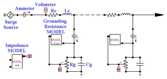
Figure 4.
Example of ATP model for vertical rods.
The model block is a component of ATP-DRAW that allows writing an algorithm [52], and oversees the control of the time variable shunt resistance. For the control of the grounding resistance, a model block is designed, which changes the value of the effective radius where the ionization is produced. In addition, an impedance model is used to show the behavior of the impulse grounding impedance. This is calculated using the relation between the ground potential rise and the injected current, both as a function of time.
The shunt capacitance is considered constant during the simulations due to their small variation compared with the resistive components. Therefore, the assumption about only the grounding resistance varying in function of time is considered [51]. This assumption decreases the complexity and the overall time of the simulations.
There are some factors that affect the impulse grounding impedance of a vertical rod such as the dimensions of the grounding system, the soil resistivity, the peak reached by the surge current and the electric field of the soil [53].
The behavior of impulse grounding impedance as a function of the electrode length, when setting the values of the soil resistivity at 500 Ωm, critical electric field at 10 kV/cm, current peak at 50 kA and waveform at 0.25/100 μs, is shown in Figure 5. This impulse waveform represents lightning current, namely, a subsequent negative stroke.
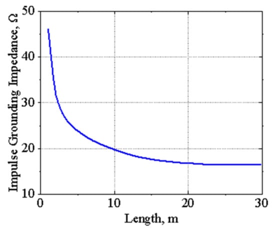
Figure 5.
Influence of length on the impulse grounding impedance of a vertical rod with soil resistivity of 500 Ωm, critical electric field of 10 kV/cm, current peak of 50 kA and waveform 0.25/100 μs.
It may be noted that the impulse grounding impedance decreases when the length of the electrode increases. In addition, the impulse grounding impedance becomes saturated after reaching a certain length. This is because the inductive effect of the vertical rod makes the leakage currents along the conductor non-uniform, and this inequality increases when the length of the conductor increases.
The results of the behavior of the impulse grounding impedance as a function of the soil resistivity is shown in Figure 6. The impulse grounding impedance increases when the soil resistivity increases in an almost linear relationship.
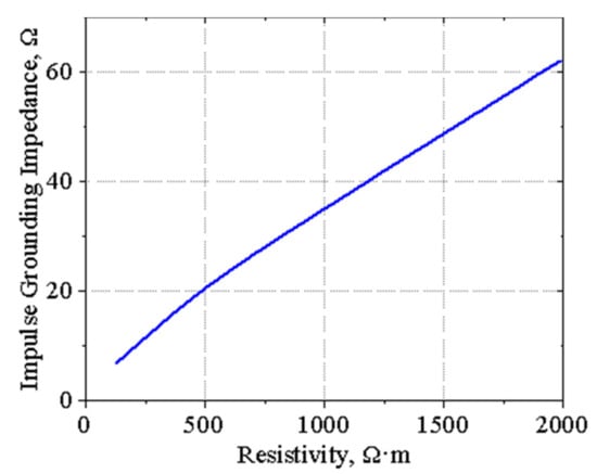
Figure 6.
Influence of the resistivity on the impulse grounding impedance of a vertical rod of 10 m, critical electric field of 10 kV/cm, current peak of 50 kA and waveform of 0.25/100 μs.
The surge as lightning can take different peak values, according to the IEC 62305 [54]. Therefore, the impulse grounding impedance as a function of the peak of the injected surge current is as shown in Figure 7. The set values were a length of 10 m, soil resistivity of 500 Ωm, critical electric field of 10 kV/cm and current waveform of 1/200 μs. This impulse waveform represents lightning current, namely, the first negative short stroke. Therefore, the impulse grounding impedance decreases when the peak of the injected current increases.
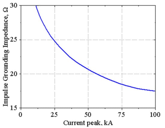
Figure 7.
Influence of the current peak on the impulse grounding impedance of a vertical rod of 10 m, soil resistivity of 500 Ωm, critical electric field of 10 kV/cm and current waveform of 1/200 μs.
The behavior of the impulse grounding impedance as a function of the critical electric field of the soil is shown in Figure 8. It may be seen that the impulse grounding impedance increases when the critical electric field of the soil increases.
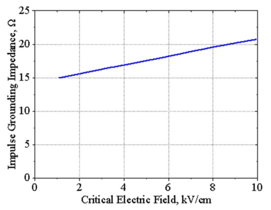
Figure 8.
Influence of the critical electric field on the impulse grounding impedance of a vertical rod of 10 m, soil resistivity of 500 Ωm, current peak of 50 kA and waveform of 0.25/100 μs.
An example of circuit model for a 1 × 1 mesh is shown in Figure 9. In case of the 1 × 1 mesh, each rod that composes the square mesh is represented as a horizontal rod. Therefore, each rod can be implemented as non-uniformly lumped parameters in a transmission line model. In this case, the mutual coupling between conductors is considered and it is represented as a controlled voltage source in the leakage branch.
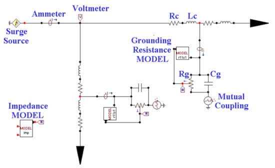
Figure 9.
Example of ATP model for mesh simulations.
The behavior of the impulse grounding impedance of a 1 × 1 mesh is similar to a vertical rod, but it differs, especially in the values of the magnitude, because the 1 × 1 mesh takes up more area in the ground. The impulse waveform used in this case is 1/200 μs. The behavior of the impulse grounding impedance is similar that the single rod, but they differ due to the change of the impulse waveform.
The behavior of the impulse grounding impedance as a function of the mesh side length is shown in Figure 10. It may be noted that the impulse grounding impedance decreases when the side length of the 1 × 1 mesh increases. In addition, the resistivity becomes constant for bigger areas of the mesh.
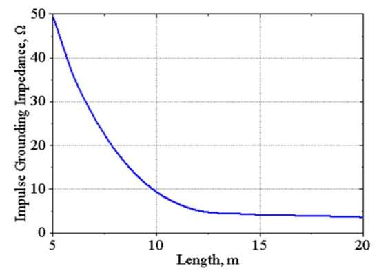
Figure 10.
Influence of the length on the impulse grounding impedance of a 1 × 1 mesh with soil resistivity of 500 Ωm, critical electric field of 10 kV/cm, current peak of 100 kA and 1/200 μs waveform.
The behavior of the impulse grounding impedance in function of soil resistivity, with set values of 10 m, critical electric field of 10 kV/cm, current peak of 50 kA and waveform 1/200 μs, is shown in Figure 11. It may be noted that the impulse grounding impedance increases when the soil resistivity increases. In addition, the curve shows an almost linear relationship between the two variables.
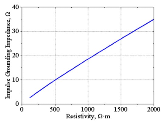
Figure 11.
Influence of the soil resistivity on the impulse grounding impedance of a 1 × 1 mesh of 10 m, critical electric field of 10 kV/cm, current peak of 50 kA and 1/200 μs waveform.
The behavior of the impulse grounding impedance as a function of the peak of the injected current is shown in Figure 12. It may be noted that the impulse grounding impedance decreases when the peak of the injected current of the 1 × 1 mesh increases.
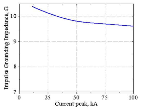
Figure 12.
Influence of the current peak on the impulse grounding impedance of a 1 × 1 mesh of 10 m, soil resistivity of 500 Ωm, critical electric field of 10 kV/cm and 1/200 μs waveform.
The behavior of the impulse grounding impedance as a function of the critical electric field of the soil is shown in Figure 13. It may be noted that the impulse grounding impedance increases slightly when the critical electric field of the soil for the 1 × 1 mesh increases.

Figure 13.
Influence of the critical electric field on the impulse grounding impedance of a 1 × 1 mesh of 10 m, soil resistivity of 500 Ωm, current peak of 100 kA and 1/200 μs waveform.
4. Example of Model Validations
For the validation of the circuit model, the results of the simulation made in ATPDraw can be compared with the experimental measurements using several wave tail shapes of applied current made, e.g., in [55]. The measured results were obtained by injecting a surge current to a driven rod vertically buried.
Table 1 shows the electrical parameters of the vertical rod and the soil, and they are used for simulating the conditions of the measured experiment.

Table 1.
Parameters of the electrode and soil for the vertical rod.
The experimental measurements made with the vertical rod are shown in [56]. The analysis assumptions consist of the injected current having a peak of 2.35 kA, approximately, with a waveform of 3/9 μs and ground potential rise 130 kV, approximately [56]. The impulse grounding impedance starts at a zero value and increases in value very fast in a time of 1.0 μs, approximately; this behavior is produced by the inductive effect zone. After that, the grounding impedance decreases to the minimum value, which is produced by the ionization of the soil. Finally, the grounding impedance increases, which is due to the deionization of the soil [50].
Table 2 shows the values used in the ATPDraw tool for the circuit model, which are set to simulate the conductor and soil parameters.
Table 2.
Parameters of vertical rod and soil in the ATPdraw tool.
For purposes of simulation, a surge current source of a double exponential waveform is used as the injected current to the vertical rod of the experimental case. The equation that represents the double exponential waveform is [57]; the value of α is 25,000 and β is 320,000 with a peak value of 2.35 kA. The simulated waveform of the injected current is shown in Figure 14.
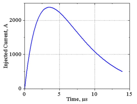
Figure 14.
Injected current to the vertical rod of 1.5 m.
Figure 15 shows the transient ground potential rise produced in the vertical rod when the surge current is applied. The waveform shapes are almost like the injected current, reaching a peak value of 119.8 kV when the critical electric field is 8 kV/cm and 127.9 kV when the critical electric field is 10 kV/cm. It may be noted that the percentage error of the maximum transient ground potential rise compared with the experimental measurements is 7.8% for 8 kV/cm and 1.6% for 10 kV/cm. Furthermore, Figure 15 shows the transient ground potential rise produced in the vertical rod when the soil ionization is not considered. The maximum value reached is 219 KV, approximately. Therefore, this result is 80% higher that the experimental value.
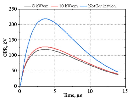
Figure 15.
Transient ground potential rise produced in a vertical rod of 1.5 m, soil resistivity of 160 Ωm and a peak current of 2.35 kA.
Figure 16 shows the grounding impedance response when the surge current is applied to the vertical rod. The grounding impedance increases during 1 μs reaching a value of 61.8 Ω for a critical electric field of 8 kV/cm and 65.7 Ω for a critical electric field of 10 kV/cm, and then decreases when the current flowing through the rod increases. After the surge current reaches its maximum value, the grounding impedance starts increasing. In addition, the impulse grounding impedance is calculated giving a value of 51.0 Ω for a critical electric field of 8 kV/cm and 54.4 Ω for a critical electric field of 10 kV/cm. The percentage error of the grounding impedance between the simulation and the experimental measurement is 7.3% for a critical electric field of 8 kV/cm and 1.0% for 10 kV/cm.
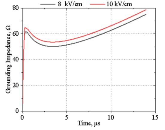
Figure 16.
Grounding impedance produced in a vertical rod of 1.5 m, soil resistivity of 160 Ωm and a peak current of 2.35 kA.
Figure 17 shows the behavior of the radius of the ionized zone of the soil. When ionization is not produced in the soil, the equivalent radius is equal to the conductor radius. Then, the ionization radius increases reaching a maximum value of 46.9 and 37.6 mm for a critical electric field of 8 and 10 kV/cm, respectively, during the peak of the surge current. Finally, when the surge current decreases, the equivalent radius of the ionized zone decreases.
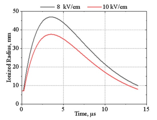
Figure 17.
Equivalent cylindrical radius produced for soil ionization in a vertical rod of 1.5 m, soil resistivity of 160 Ωm and peak current of 2.35 kA.
5. Conclusions
The present paper gives a comprehensive overview of modelling of standard grounding system configurations under surge conditions. The considerations are made on the basis of models implemented in ATP-EMTP/ATPDraw.
It is important to mention that in general, industrial grounding systems are more complex that a simple rod or a 1 × 1 m mesh. However, the methodology discussed can be applied to the development of all kinds of earthing system models.
For simulation purposes and model development, it is important to stress that the non-linear response of the grounding response can be affected by some parameters of the soil, the rod and the impulse current that flows inside the grounding systems, notably:
- −
- peak of the impulse current;
- −
- length of the rod that composes the grounding system;
- −
- resistivity of the soil;
- −
- critical electric field of the soil.
The impact of such parameters will be visible in the results of computer simulations.
The results of this paper demonstrate a good agreement between simulations and experimental measurements. The computer simulation results show an acceptable error of 7% at most in the impulse grounding response.
Author Contributions
Conceptualization, T.K. and M.C.; Formal analysis, T.K. and M.C.; Investigation, M.C.; Methodology, T.K. and M.C.; Supervision, T.K. All authors have read and agreed to the published version of the manuscript.
Funding
This research was funded in part by the Warsaw University of Technology, and Universidad Técnica Estatal de Quevedo.
Institutional Review Board Statement
Not applicable.
Informed Consent Statement
Not applicable.
Data Availability Statement
Not applicable.
Acknowledgments
The paper has been prepared in the frame of international cooperation between Poland and Ecuador. The authors wish to express their gratefulness to the authorities of Warsaw University of Technology and government of Ecuador, namely SENESCYT for related support.
Conflicts of Interest
The authors declare no conflict of interest.
References
- Tete, P.; Hasnaoui, F.S.; Georges, S. Analysis of the lightning transient response of the grounding system of large wind farms. In Proceedings of the 2020 5th International Conference on Renewable Energies for Developing Countries (REDEC), Marrakech, Morocco, 29–30 June 2020; pp. 1–6. [Google Scholar] [CrossRef]
- Kisielewicz, T.; Blicharz, G.; Mazzetti, C.; Mosti, G.; Tofani, A.; De Carli, D.; Montarese, V. Technical and legal aspects of critical infrastructure protection. Law Action 2018, 36, 65–75. [Google Scholar]
- Mitolo, M. On the New Terminology Introduced in Std. IEEE P3003.2 “Recommended Practice for Equipment Grounding and Bonding in Industrial and Commercial Power Systems”. In Proceedings of the 2015 IEEE/IAS 51st Industrial & Commercial Power Systems Technical Conference (I&CPS), Calgary, AB, USA, 6–8 May 2015; pp. 1–5. [Google Scholar]
- Blicharz, G.; Kisielewicz, T. Legal aspects of governing the commons against technical challenges of smart city development. Forum Praw. 2017, 39, 34. [Google Scholar]
- Kisielewicz, T.; Blicharz, G. An interdisciplinary approach to service continuity provision of power systems. In Proceedings of the Medial International Scientific Conference of the Series: Decisions in Situations of Endangerment, Wroclaw, Poland, 23 November 2017; General Tadeusz Kościuszko Military University of Land Forces in Wrocław: Wrocław, Poland, 2017. [Google Scholar]
- Jambak, M.I.; Ahmad, H. Measurement of grounding system resistance based on ground high frequency behavior for different soil type. In Proceedings of the 2000 TENCON Intelligent Systems and Technologies for the New Millennium (Cat. No. 00CH37119), Kuala Lumpur, Malaysia, 24–27 September 2000; Volume 3, pp. 207–211. [Google Scholar] [CrossRef]
- Lian, D.; Bo, Z.; Jinliang, H.; Leishi, X.; Qian, L. Experimental study on transient characteristics of grounding grid for substation. In Proceedings of the 2016 33rd International Conference on Lightning Protection (ICLP), Estoril, Portugal, 25–30 September 2016; pp. 1–6. [Google Scholar] [CrossRef]
- Kisielewicz, T.; Lo Piparo, G.B.; Mazzetti, C.; Fiamingo, F. Impact of an extended grounding system on the factors affecting selection of an SPD system for apparatus safety. Electr. Rev. 2016, 92, 51–53. [Google Scholar] [CrossRef][Green Version]
- Lo Piparo, G.B.; Kisielewicz, T.; Mazzetti, C.; Fiamingo, F. Protection of apparatus against lightning surge in an extended earthing arrangement. In Proceedings of the 16 IEEE International Conference on Environment and Electrical Engineering, Florence, Italy, 7–10 June 2016. [Google Scholar]
- Lo Piparo, G.B.; Kisielewicz, T.; Fiamingo, F.; Mazzetti, C. Influence of grounding conditions on apparatus protection by means of SPD. In Proceedings of the XXIII International Conference on Electromagnetic Disturbances (EMD 2015), Białystok, Poland, 9–11 September 2015. [Google Scholar]
- Yang, S.; Zhou, W.; Huang, J.; Yu, J. Investigation on Impulse Characteristic of Full-Scale Grounding Grid in Substation. IEEE Trans. Electromagn. Compat. 2018, 60, 1993–2001. [Google Scholar] [CrossRef]
- Kisielewicz, T.; Lo Piparo, G.B.; Mazzetti, C.; Fiamingo, F. Factors influencing the probability of an apparatus damage in an extended earthing arrangement. In Proceedings of the International Conference on Lightning Protection 2016, Estoril, Portugal, 25–30 September 2016. [Google Scholar]
- Permal, N.; Osman, M.; Kadir, M.Z.A.A.; Ariffin, A.M. Review of Substation Grounding System Behavior under High Frequency and Transient Faults in Uniform Soil. IEEE Access 2020, 8, 142468–142482. [Google Scholar] [CrossRef]
- Sekioka, S. Discussion of current dependent grounding resistance using an equivalent circuit considering frequency-dependent soil parameters. In Proceedings of the 2016 33rd International Conference on Lightning Protection (ICLP), Estoril, Portugal, 25–30 September 2016; pp. 1–6. [Google Scholar] [CrossRef]
- Gazzana, D.S.; Tronchoni, A.B.; Bretas, A.S.; Pulz, L.T.; Ferraz, R.G.; Telló, M. A Transmission Line Modeling (TLM) Algorithm to Evaluate Grounding Grids Including Soil Ionization. In Proceedings of the 2020 IEEE International Conference on Environment and Electrical Engineering and 2020 IEEE Industrial and Commercial Power Systems Europe (EEEIC/I & CPS Europe), Madrid, Spain, 9–12 June 2020; pp. 1–4. [Google Scholar] [CrossRef]
- Yassin, S.; El Dein, A.Z. Transient performance of horizontal grounding electrode under soil ionization effect. In Proceedings of the 2017 Nineteenth International Middle East Power Systems Conference (MEPCON), Cairo, Egypt, 19–21 December 2017; pp. 796–801. [Google Scholar] [CrossRef]
- Towne, H.M. Impulse characteristics of driven grounds. Gen. Electr. Rev. 1929, 31, 605–609. [Google Scholar]
- Ivonin, V.V. Experimental Investigation of Impulse Resistance of Different Type Grounding Electrodes. In Proceedings of the 2020 International Multi-Conference on Industrial Engineering and Modern Technologies (FarEastCon), Vladivostok, Russia, 6–7 October 2020; pp. 1–4. [Google Scholar] [CrossRef]
- Zhang, F.; Tanaka, H.; Baba, Y.; Nagaoka, N. FDTD surge simulation of a vertical grounding rod considering soil ionization. In Proceedings of the 2016 Asia-Pacific International Symposium on Electromagnetic Compatibility (APEMC), Shenzen, China, 18–21 May 2016; pp. 260–262. [Google Scholar] [CrossRef]
- Gao, Y.Q. Research on Mechanism of Soil Breakdown and Transient Characteristics of Grounding Systems. Ph.D. Thesis, Tsinghua University, Beijing, China, 2003. [Google Scholar]
- Fajingbesi, F.E.; Shahida Midi, N.; Elsheikh, E.M.A.; Hajar Yusoff, S.; Khan, S.; Azman, A.W. Induced Current Distribution in 3D Soil Model as Lightning Impulse Discharge Strike Earth Surface. In Proceedings of the 2019 9th International Conference on Power and Energy Systems (ICPES), Perth, Australia, 10–12 December 2019; pp. 1–6. [Google Scholar] [CrossRef]
- Kumar, A.S.; Manickavasagam, K. Mathematical modelling of dynamic soil resistivity under transient conditions. In Proceedings of the 2017 International Conference on Technological Advancements in Power and Energy (TAP Energy), Kollam, India, 21–23 December 2017; pp. 1–6. [Google Scholar] [CrossRef]
- Kherif, O.; Chiheb, S.; Teguar, M.; Mekhaldi, A.; Harid, N. Time-Domain Modeling of Grounding Systems’ Impulse Response Incorporating Nonlinear and Frequency-Dependent Aspects. IEEE Trans. Electromagn. Compat. 2018, 60, 907–916. [Google Scholar] [CrossRef]
- Mokhtari, M.; Abdul-Malek, Z.; Gharehpetian, G.B. A critical review on soil ionisation modelling for grounding electrodes. Arch. Electr. Eng. 2016, 65, 449–461. [Google Scholar] [CrossRef]
- Chiheb, S.; Kherif, O.; Teguar, M.; Mekhaldi, A. Incorporation of soil ionization and mutual coupling in transient study of horizontal grounding electrode using TLM. In Proceedings of the 2017 5th International Conference on Electrical Engineering—Boumerdes (ICEE-B), Boumerdes, Algeria, 29–31 October 2017; pp. 1–4. [Google Scholar] [CrossRef]
- Datsios, Z.G.; Mikropoulos, P.N.; Staikos, E.T.; Tsovilis, T.E.; Vlachopoulos, D.; Ganatsios, S. Laboratory Measurement of the Impulse Characteristics of Wet Sand. In Proceedings of the 2020 IEEE International Conference on Environment and Electrical Engineering and 2020 IEEE Industrial and Commercial Power Systems Europe (EEEIC/I & CPS Europe), Madrid, Spain, 9–12 June 2020; pp. 1–6. [Google Scholar] [CrossRef]
- Kim, H.-G.; Lee, B.-H. Characteristics of Impulse Discharges in Wet Soil. Trans. Korean Inst. Electr. Eng. 2020, 66, 363–369. [Google Scholar] [CrossRef]
- Kun, L.; Chuan, W.; Huilian, S. Estimation of critical electric field intensity of soil ionization base on the ohm’s law. In Proceedings of the 2016 Asia-Pacific International Symposium on Electromagnetic Compatibility (APEMC), Shenzen, China, 18–21 May 2016; pp. 53–55. [Google Scholar] [CrossRef]
- Oettle, E.E. A new general estimation curve for predicting the impulse impedance of concentrated earth electrodes. IEEE Paper. In Proceedings of the IEEE-PES 1987 Summer Meeting, San Francisco, CA, USA, 12–17 July 1987. [Google Scholar]
- IEEE Working Group. Estimating lightning performance of transmission lines II- updates to analytical models. IEEE Trans. Power Deliv. 1993, 8, 1254–1267. [Google Scholar] [CrossRef]
- Shariatinasab, R.; Ghayur, J.; Safar, J.; Gholinezhad, J.; He, J. Analysis of Lightning-Related Stress in Transmission Lines Considering Ionization and Frequency-Dependent Properties of the Soil in Grounding Systems. IEEE Trans. Electromagn. Compat. 2020, 62, 2849–2857. [Google Scholar] [CrossRef]
- Trlep, M.; Jesenik, M.; Beković, M.; Hamler, A. Nonlinear Transient Finite Element Analysis of Grounding Systems. In Proceedings of the 2019 19th International Symposium on Electromagnetic Fields in Mechatronics, Electrical and Electronic Engineering (ISEF), Nancy, France, 29–31 August 2019; pp. 1–2. [Google Scholar] [CrossRef]
- Gazzana, D.S.; Bretas, A.S.; Thomas, D.W.P.; Christopoulos, C. A hybrid method to represent the soil ionization phenomenon in impulsive grounding systems. In Proceedings of the 2016 IEEE Conference on Electromagnetic Field Computation (CEFC), Miami, FL, USA, 13–16 November 2016; p. 1. [Google Scholar] [CrossRef]
- Garma, T.; Sesnic, S.; Poljak, D.; Blajic, M. Impulse impedance of the horizontal grounding electrode: Experimental analysis versus full-wave computational model. In Proceedings of the 2016 24th International Conference on Software, Telecommunications and Computer Networks (SoftCOM), Split, Croatia, 22–24 September 2016; pp. 1–4. [Google Scholar] [CrossRef]
- Safar, J.G.; Shariatinasab, R.; He, J. Comprehensive Modeling of Grounding Electrodes Buried in Ionized Soil Based on MoM-HBM Approach. IEEE Trans. Power Deliv. 2020, 35, 1390–1398. [Google Scholar] [CrossRef]
- Zhang, F.; Tanaka, H.; Baba, Y.; Nagaoka, N. Soil ionization effects on surge characteristics of grounding electrodes. IEEJ Trans. Electr. Electron. Eng. 2019, 14, 1609–1616. [Google Scholar] [CrossRef]
- De Oliveira, R.M.; Fujiyoshi, D.M. Finite-difference time-domain modeling of multi-stage soil ionization with residual resistivities—Part I: Theoretical background and the proposed FDTD formulation. Electr. Power Syst. Res. 2020, 184, 106300. [Google Scholar] [CrossRef]
- De Oliveira, R.M.; Fujiyoshi, D.M. Finite-difference time-domain modeling of multi-stage soil ionization with residual resistivities—Part II: Numerical validation. Electr. Power Syst. Res. 2020, 184, 106299. [Google Scholar] [CrossRef]
- Gazzana, D.S.; Tronchoni, A.B.; Leborgne, R.C.; Bretas, A.S.; Thomas, D.W.P.; Christopoulos, C. An Improved Soil Ionization Representation to Numerical Simulation of Impulsive Grounding Systems. IEEE Trans. Magn. 2018, 54, 7200204. [Google Scholar] [CrossRef]
- Chen, H.; Du, Y. Lightning Grounding Grid Model Considering Both the Frequency-Dependent Behavior and Ionization Phenomenon. IEEE Trans. Electromagn. Compat. 2019, 61, 157–165. [Google Scholar] [CrossRef]
- Wen-Rong, S.; Chen-Zhao, F.; Lu, C.; Qi-Yu, L.; Hai-Long, B.; Peng, Y. Research on Field Test of Impulse Grounding Impedance for Small Substation. In Proceedings of the 2018 International Conference on Smart Grid and Electrical Automation (ICSGEA), Singapore, 27–30 April 2018; pp. 159–162. [Google Scholar] [CrossRef]
- Chiheb, S.; Kherif, O.; Teguar, M.; Mekhaldi, A. Transient behavior of vertical grounding electrode under impulse current. In Proceedings of the 2017 5th International Conference on Electrical Engineering (ICEE-B), Boumerdes, Algeria, 29–31 October 2017; pp. 1–5. [Google Scholar] [CrossRef]
- Messaoudi, H.E.; Kherif, O.; Chiheb, S.; Teguar, M.; Mekhaldi, A. Modelling of Vertical Ground Electrode under Lightning Transient. In Proceedings of the 2019 19th International Symposium on Electromagnetic Fields in Mechatronics, Electrical and Electronic Engineering (ISEF), Nancy, France, 29–31 August 2019; pp. 1–2. [Google Scholar] [CrossRef]
- Djamel, I.; Slaoui, F.H.; Georges, S. Transient response of grounding systems under impulse lightning current. In Proceedings of the 2016 Electric Power Quality and Supply Reliability (PQ), Tallinn, Estonia, 29–31 August 2016; pp. 71–75. [Google Scholar] [CrossRef]
- Sekioka, S. Frequency and Current-Dependent Grounding Resistance Model for Lightning Surge Analysis. IEEE Trans. Electromagn. Compat. 2019, 61, 419–425. [Google Scholar] [CrossRef]
- Djamel, I.; Slaoui, F.H.; Georges, S. Analysis of the Transient Behavior of Grounding Systems with Consideration of Soil Ionization. In Proceedings of the 2018 15th International Conference on the European Energy Market (EEM), Lodz, Poland, 27–29 June 2018; pp. 1–5. [Google Scholar] [CrossRef]
- He, J.; Gao, Y.; Zeng, R.; Zou, J.; Liang, X.; Zhang, B.; Lee, J.; Chang, S. Effective length of counterpoise wire under lightning current. IEEE Trans. Power Deliv. 2005, 20, 1585–1591. [Google Scholar] [CrossRef]
- Grcev, L. Modeling of Grounding Electrodes under Lightning Currents. IEEE Trans. Electromagn. Compat. 2009, 51, 559–571. [Google Scholar] [CrossRef]
- Rüdenberg, R. Grounding principles and practice I—Fundamental considerations on ground currents. Electr. Eng. 1945, 64, 1–13. [Google Scholar] [CrossRef]
- Meliopoulos, A.P.; Moharam, M.G. Transient characteristics of grounding system. IEEE Trans. Power Appar. Syst. 1983, 102, 389–399. [Google Scholar] [CrossRef]
- He, J.; Zeng, R.; Zhang, B. Methodology and Technology for Power System Grounding; Wiley: Singapore, 2013. [Google Scholar]
- Høidalen, H.K.; Prikler, L.; Peñaloza, F. ATPDRAW—Version 7.2—For Windows, Users’ Manual; Norwegian University of Technology: Trondheim, Norway, 2020. [Google Scholar]
- Zeng, R.; Gong, X.; He, J.; Zhang, B.; Gao, Y. Lightning Impulse Performances of Grounding Grids for Substations Considering Soil Ionization. IEEE Trans. Power Deliv. 2008, 23, 667–675. [Google Scholar] [CrossRef]
- IEC 62305-1; Edition 2.0 2010-12. Protection against Lightning—Part 1: General Principles. IEC: Geneva, Switzerland, 2010.
- Sekioka, S.; Sonoda, T.; Ametani, A. Experimental study of currentdependent grounding resistances of rod electrode. IEEE Trans. Power Deliv. 2005, 20, 1569–1576. [Google Scholar] [CrossRef]
- Sekioka, S.; Lorentzou, M.I.; Philippakou, M.P.; Prousalidis, J.M. Current-dependent grounding resistance model based on energy balance of soil ionization. IEEE Trans. Power Deliv. 2006, 21, 194–201. [Google Scholar] [CrossRef]
- Jia, W.; Xiaoqing, Z. Double-Exponential Expression of Lightning Current Waveforms. In Proceedings of the 2006 4th Asia-Pacific Conference on Environmental Electromagnetics, Dalian, China, 1–4 August 2006; pp. 320–323. [Google Scholar] [CrossRef]


Publisher’s Note: MDPI stays neutral with regard to jurisdictional claims in published maps and institutional affiliations. |
© 2022 by the authors. Licensee MDPI, Basel, Switzerland. This article is an open access article distributed under the terms and conditions of the Creative Commons Attribution (CC BY) license (https://creativecommons.org/licenses/by/4.0/).