Abstract
A fiber-optic gyroscope (FOG) with lower precision but higher cost advantage is typically selected according to working conditions and engineering budget. Thermal drift is the main factor affecting FOG precision. External thermal calibration methods by algorithms can effectively weaken the influence of thermal drift. This paper presents a thermal calibration method of a two-dimensional N-order polynomial (TDNP) and compares it with artificial neural network (ANN) methods to determine a software FOG thermal calibration method for landslide displacement monitoring. The TDNP thermal calibration coefficient matrix was established, and the thermal calibration capability of the TDNP method with different orders N was evaluated on the basis of error analysis. The ANN model with 1 to 18 hidden neural layers was established on the basis of LM, BR, and SCG algorithms to choose a suitable ANN. Finally, the mean absolute errors of FOG thermal calibration through the TDNP with different orders and the LM were compared. This method was applied in the Huangtupo landslide area, China. The results highlight that the TDNP method with order 5 had better performance and satisfied the requirements of landslide displacement monitoring. The research results can compensate for the lack of adaptability of the FOG thermal calibration method in landslide displacement monitoring.
1. Introduction
1.1. Monitoring Principle Based on the Inertial Measurement System
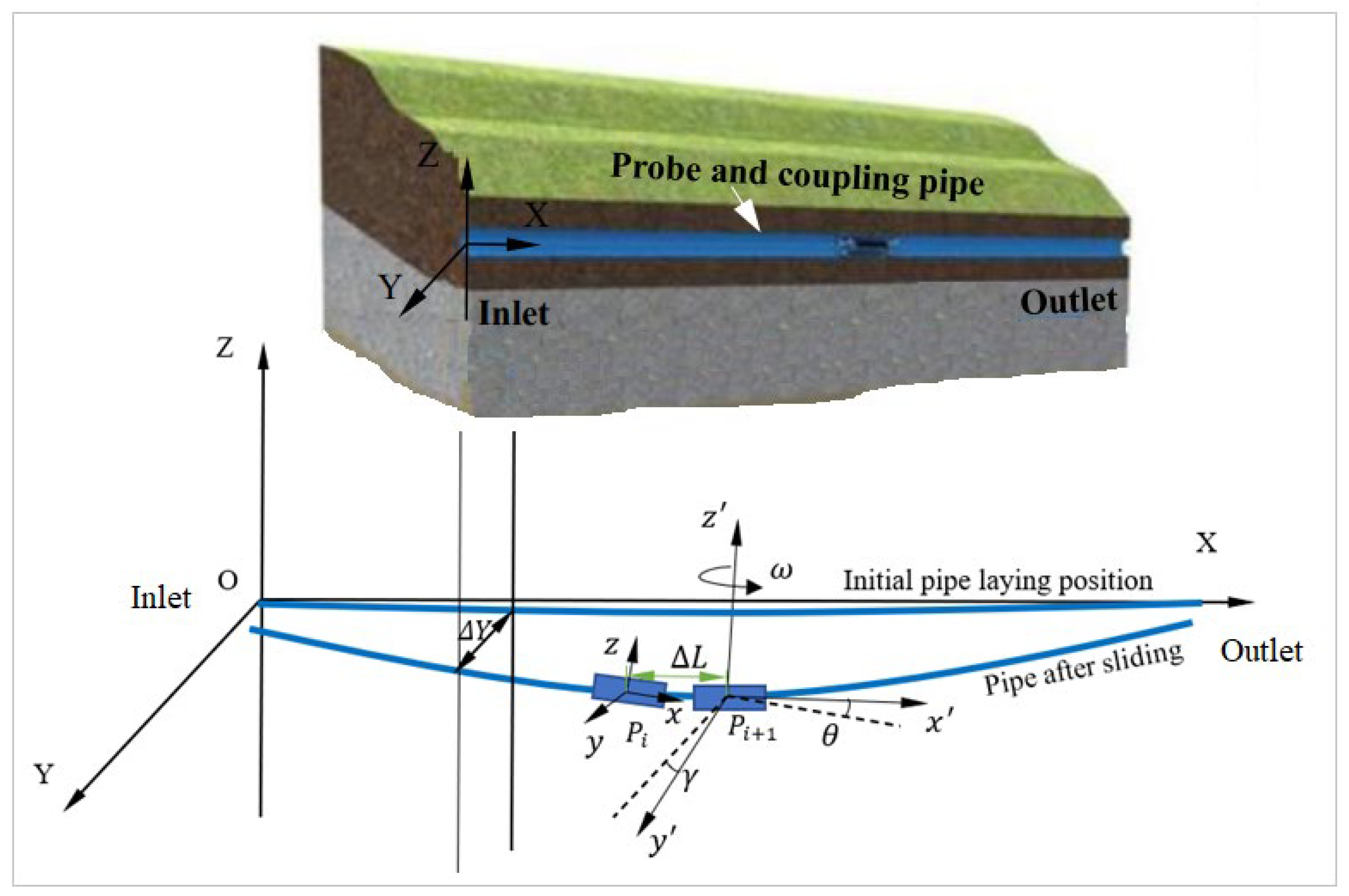
Landslides, collapse, debris flow, and ground deformation are common geological disasters in the field of geotechnical engineering. Among them, the landslide is a highly destructive geological disaster, which is widely distributed around the globe. Monitoring the three-dimensional continuous displacement change of a landslide profile can provide data support for analyzing the landslide formation mechanism, failure mode, sliding zone identification, and prediction of landslide disasters. The traditional inclinometer for landslide displacement adopts the point measurement method, which cannot measure the horizontal continuous displacement below the surface. To obtain the continuous displacement data, our group coupled landslide displacement and deformation along a horizontal survey line using a flexible pipe [1]. Figure 1 shows the principle of landslide displacement measurement based on the inertial measurement system. A measuring probe moves from the inlet to the outlet at an almost constant speed and simultaneously detects the three-dimensional trajectory of a coupling pipe at the same time. When a coupling pipe slides with a landslide, its three-dimensional trajectory changes accordingly, and the horizontal position difference Δ Y obtained by two trajectory measurements of a coupling pipeline before and after shows the horizontal displacement distribution along a survey line. Similarly, the vertical displacement can be obtained. denotes any sampling point. The initial attitude at the coupling pipe inlet is measured, and then the sampling interval distance ∆ L and angle of pitch , roll , and yaw are detected while the probe moves; finally, the three-dimensional trajectory of the coupling pipe is calculated on the basis of the initial attitude and these four parameters. The angles of pitch and yaw are measured by accelerometers and gyroscopes, and the distances between two sampling points are measured by a Hall sensor and a micro-magnetic encoder.
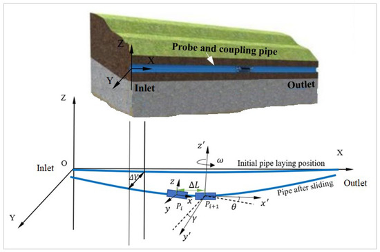
Figure 1.
Principle of landslide displacement measurement.
In the process of landslide displacement measurement, the change in yaw angle is usually smaller than the change in roll angle, which means that the yaw angular rate is lower. If a sensor can sense the yaw angular rate, it can satisfy the requirements of landslide displacement measurement, assuming that the movement of landslide mass causes the trajectory of a coupling pipe to turn more than one degree, the measurement time is not more than three minutes, and the requirement for the resolution of an angular rate sensor is at least 0.005 deg/s.
The diameter of a coupling pipe is limited to ensure its flexibility. To meet the requirements of the measurement resolution and coupling pipe diameter, and considering the cost performance, two fiber-optic gyroscopes (FOGs) were selected, numbered 070076 and 070077. Their bias stability is 2 deg/h, their temperature range is between −40 °C and 60 °C, and their angular rate range is ±50 deg/s. The feasibility verification of the thermal calibration methods in the research process was on the basis of the output data of the two gyroscopes at different temperatures and rotation speeds. However, it must be emphasized that the research is not limited to these two gyroscopes. It is suitable for thermal calibration of any angular rate sensor with random thermal drift characteristics.
The thermal drift of a FOG is random and nonlinear, which is the main factor affecting the precision of the gyroscope. The monitoring frequency of landslide displacement varies with seasons and rainfall, which means that the measuring instrument needs to be able to accurately measure within the temperature variation range of the four seasons. However, the internal temperature compensation of the FOG is insufficient, and the measurement result error caused by the temperature drift can completely exceed the change in landslide displacement. It can easily cause misjudgment of landslide stability and threaten individual lives and property safety. In addition, landslide displacement monitoring has in situ and real-time characteristics. Therefore, it is essential to develop a feasible thermal calibration method that satisfies the requirements of landslide displacement monitoring.
1.2. Methods of Thermal Calibration
Researchers and manufacturers have improved the FOG temperature performance by optimizing the fiber material, structure, and winding method and adding electronic components to suppress thermal drift [2,3,4]. However, it is difficult to eliminate the temperature error physically in engineering applications, and an FOG with lower thermal performance but higher cost advantage is usually selected according to the working conditions and engineering budget. Consequently, it is more practical to research the thermal characteristics of an FOG through experiments, to establish a thermal calibration model, and to reduce the influence of temperature by programming.
The methods of software thermal calibration are not significantly different, because of the gyroscope types. Thus, different types of gyroscopes can use the same methods. Traditional polynomial thermal calibration cannot achieve sufficient accuracy, and the parameter interpolation method was proposed to calibrate the deterministic error of a MEMS gyroscope [5]. The least-squares method (LSM) is commonly used for estimation. On the basis of the established linear correlation of the thermal drift and IFOG parameters and the least-squares error (LSE) criterion, a multivariable-combined linear model was developed to estimate the thermal drift of the IFOG [6]. However, the estimates of the drifts obtained by the LSM are not sufficiently accurate, because of gyroscope drifts jump variations. The l1-norm approximation makes it possible to identify the instants of jumps in the gyro’s readings [7]. The FOG thermal drift is primarily related to the environmental temperature, temperature gradient, and temperature change rate, which are nonlinear [8,9]. A support vector machine (SVM) was developed to overcome these problems [10]. The least-squares-support vector machine (LS-SVM) is good at solving nonlinear, small-sample learning problems and has been used in FOG thermal drift modeling and calibration to reduce the influence of temperature [9,11]. Parameters affect the calibration effect, and the artificial fish swarm algorithm (AFSA) was used to tune the parameters and optimize the LS-SVM [11].
The artificial neural network (ANN) method does not completely depend on a rigorous model. It has a strong capability to handle random data, complex nonlinear parameters, and excellent fault tolerance. A back-propagation (BP) neural network is a typical multilayer feedforward artificial neural network. The corresponding functional relationship is obtained through self-learning, and the results are stored in a BP network in the form of the connection weight of each network unit. On the basis of the BP neural network and adaptive boosting (AdaBoost) learning algorithm, a BP-AdaBoost temperature compensation method was proposed to enhance the FOG bias stability and calibration, and the results showed that the method has better performance than the traditional linear regression model, mixed linear regression model, and single BP neural network [12]. A BP neural network model with the advantage of approximating nonlinear function was developed to calibrate the FOG and MEMS gyroscope temperature error, and the results proved that the number of hidden layer neurons plays an important role in the simulation performance [13,14].
In addition, a multiscale modeling and regression method based on an improved support vector machine was proposed to improve the accuracy and calibration effect of the FOG thermal drift [15]. A fuzzy logic controller was used to realize online correction of the error due to gyroscope bias variation with temperature [16]. A gyroscope thermal calibration protocol, in that the rotation rate was estimated at any time by selecting the calibration parameters corresponding to the instantaneous temperature to the nearest 0.5 °C, was performed for human motion analysis and led to an accuracy of 0.7 deg/s [17]. A radial basis function (RBF) neural-network-based method was proposed to evaluate and compensate for the thermal drift of an FOG [18]. Particle swarm optimization (PSO) was used to estimate the calibration parameters of gyroscopes to minimize the fitness function [19].
In summary, the thermal drift of an FOG is related to the local temperature, temperature gradient, and temperature variation. The influence of the latter two factors can be ignored, and only the thermal drift caused by local temperature variation needs to be calibrated because of the limited width of the landslide and the short measurement time of approximately 3 min per hundred meters. Usually, artificial neural network (ANN) methods and traditional polynomial fitting methods are exploited in gyroscope thermal calibration. Many thermal calibration methods based on the ANN have achieved the accuracy required by the research objectives. However, the ANN method is time-consuming and more suitable for processing data through a host computer after measurement, and the training results are unstable. The traditional polynomial fitting method has a high operating speed and short time consumption. It is more suitable for directly embedded into the MCU program to process measurement data in real time and in situ. However, this method usually focuses on the relationship between the temperature and zero bias in the static state, and the thermal calibration is one-dimensional. Two-dimensional thermal calibration for the FOG, which considers the variables of angular rate and temperature simultaneously, is essential for landslide displacement monitoring. In addition, the relationship between the order of the polynomial and the calibration effect is unclear. Therefore, there is still a lack of a FOG thermal calibration method suitable for landslide displacement measurement.
This paper presents a two-dimensional N-order polynomial (TDNP) method and compares it with ANN methods to compensate for the lack of adaptability of the FOG thermal calibration method in the field of landslide displacement monitoring.
2. Thermal Calibration Experiment
Although manufacturers have also carried out thermal compensation inside the FOG and marked the scale coefficient of each gyroscope, the accuracy of the measurements calculated on the basis of the scale coefficient still cannot satisfy the above measurement conditions. Consequently, thermal calibration and other data-processing methods are required.
The soak and ramp methods are the two main approaches for thermal calibration [8]. The soak method works on the basis of the premise of stable sensor temperature, whereas the ramp method works on the basis of time-varying sensor temperature [20]. To meet the relatively high accuracy requirement of landslide monitoring, our group chose the soak method. In this way, the relationship between the real speed and the measured speed of the gyroscopes at different temperatures was obtained through experiments.
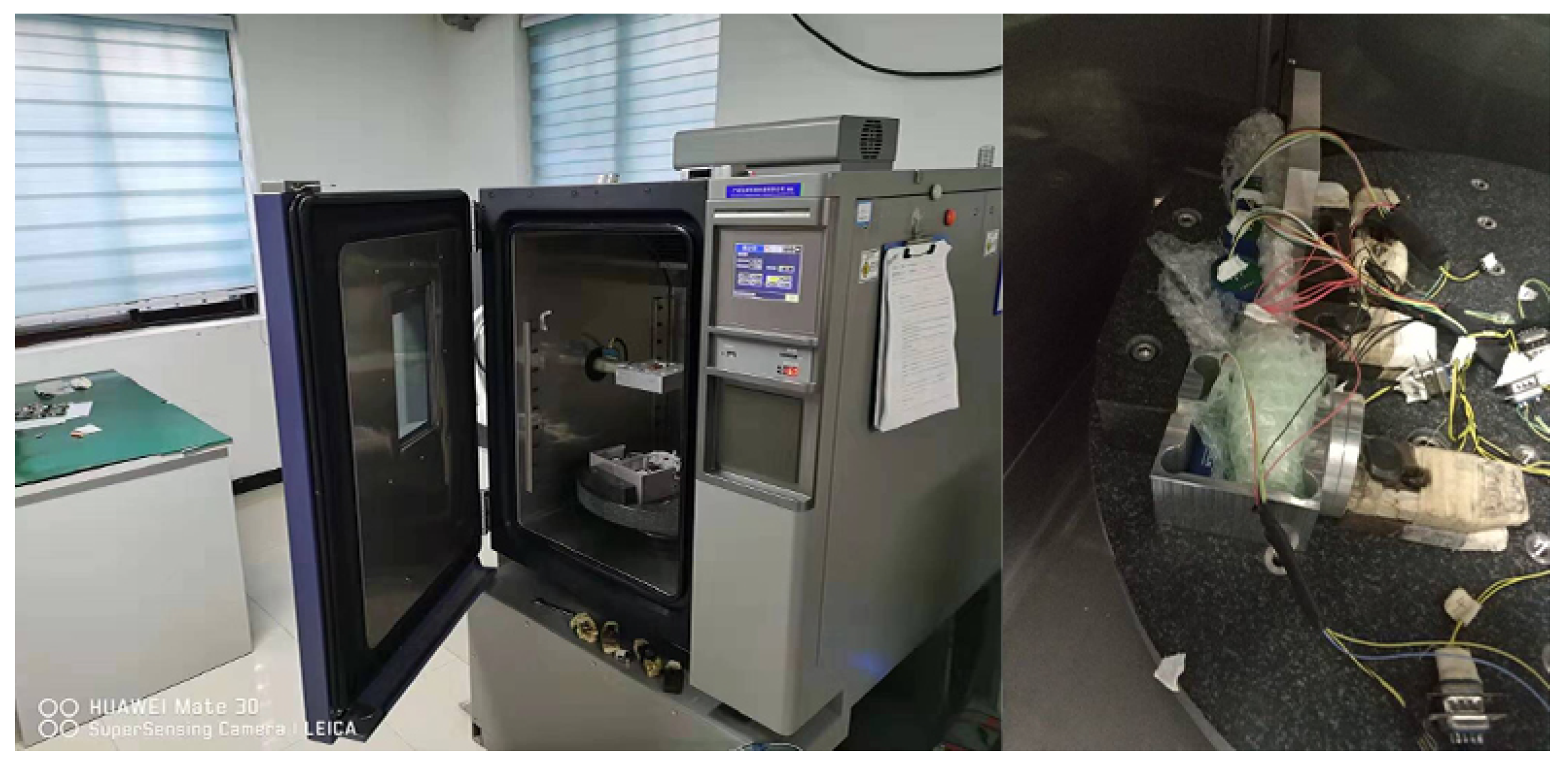
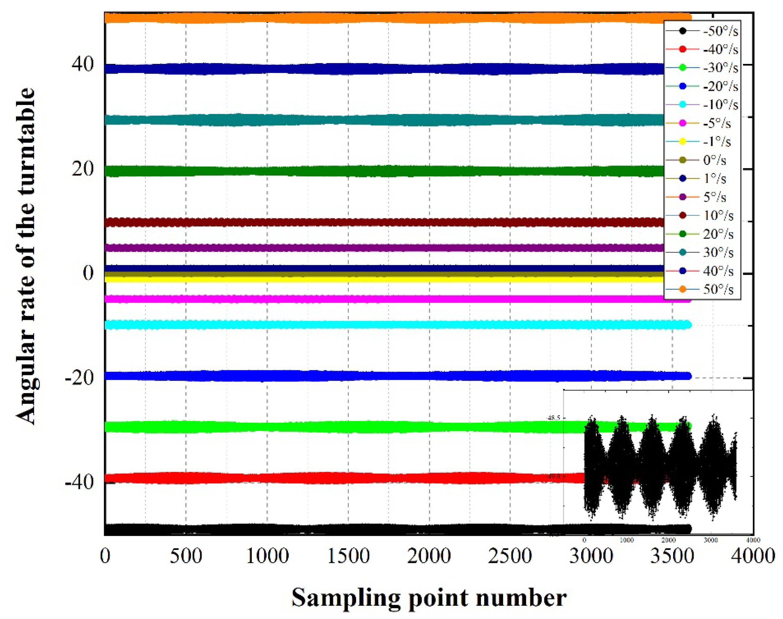
The single-axis temperature control turntable shown in Figure 2 can provide a constant-temperature environment in addition to the resolution of the angular rate up to 0.0001 deg/s. The FOGs were installed on the installation platform and rotated with the turntable at the set angular rates regarded as the true value, and the mean output of the FOGs was taken as the measurement. The site of the field test was located in the Huangtupo landslide area in Badong County, Hubei Province, China, where the temperature is generally between −10 °C and 45 °C. Considering that the temperature inside a coupling pipe is usually higher than the ambient temperature when it is close to the ground in summer, 55 °C was selected as the maximum working temperature. Accordingly, the temperatures of the experiment were controlled at −10, 10, 25, 45, and 55 °C. At the same time, the experiment was carried out at ambient temperature measured as 28 °C after natural cooling. The holding time for each temperature was set as 2 h to ensure that the internal temperature of the sensors was consistent with the set temperature during the experiment. Considering that the coupling pipe laid in advance deforms at a low level when a landslide is in the creep stage, the experimental points at around 0 deg/s were increased. The output angular rates of the turntable were controlled in the order −50, −40, −30, −20, −10, −5, −1, −0, 0, 1, 5, 10, 20, 30, 40, and 50 deg/s within the full measurement range. The minor spindle eccentricity error of the turntable affects the precision of FOG calibration. Taking the output of FOG 070076 at ambient temperature as an example, this error causes the sample data at the same angular rate to vary in the sinusoidal waveform presented in Figure 3. Therefore, sample data from at least one full turn should be collected to reduce the influence of spindle eccentricity error by offsetting the positive and negative.

Figure 2.
Thermal calibration experimental equipment.
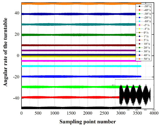
Figure 3.
Influence of turntable spindle eccentricity error on FOG 070076 output.
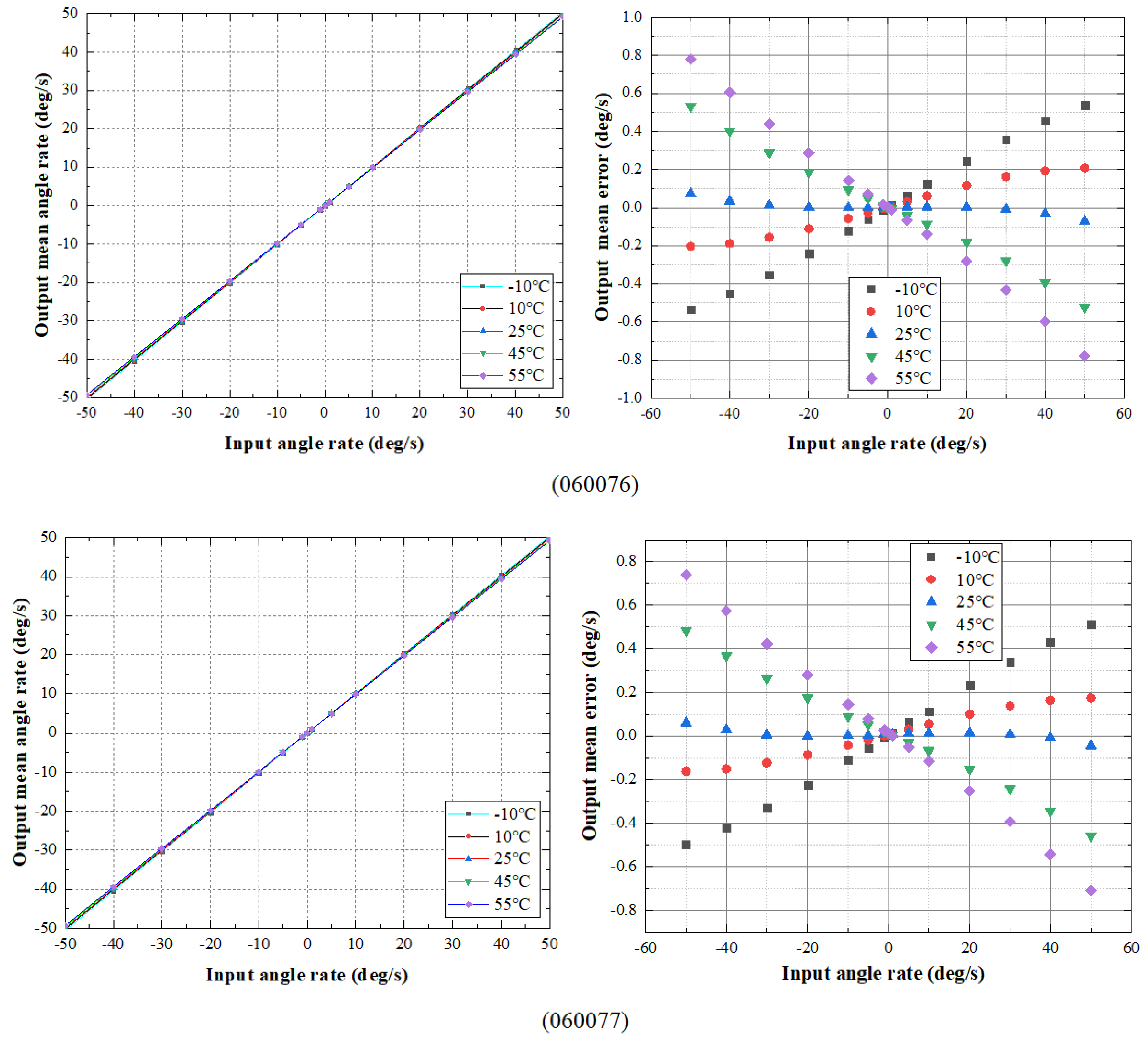
Figure 4 shows the relationship between the input angular rate of the turntable and the output mean angular rate of the two gyroscopes calculated at different temperatures according to the scale coefficient given by the manufacturer and their mean error. In the process of calculation, the amount of data collected during one rotation of the turntable at each angular rate were taken to reduce the error caused by the eccentricity of the spindle. It can be seen that the higher the input angular rate and the farther the deviation from 25 °C, the greater the measurement deviation, with the maximum deviation close to 0.8 deg/s. Such values are unacceptable for general space trajectory measurement and should be further calibrated. In addition, the degree of thermal drift is not only related to temperature, but also related to angular rate. Therefore, both temperature and angular rate should be taken into consideration in thermal calibration.
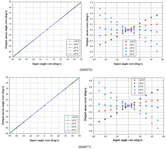
Figure 4.
Input angular rate of the turntable vs. output of the gyroscopes.
3. Thermal Calibration Based on Two-Dimensional N-Order Polynomial (TDNP)
The polynomial calibration method can reflect the drift with random and nonlinear characteristics and weaken the random error caused by the drift. The traditional polynomial fitting method focuses on the relationship between the temperature and zero bias in the static state, and the thermal calibration is one-dimensional, which cannot meet the requirement of FOG thermal calibration in landslide displacement monitoring.
The TDNP is two-dimensional. It means that the order of the polynomial is N, and the polynomial coefficient is determined by two parameters, angular rate and temperature, which are suitable for landslide survey conditions. Research on the relationship between the order of the TDNP and the thermal calibration effect is helpful in determining a TDNP model scheme with better performance.
3.1. TDNP Calibration Algorithm
The set temperature and angular rate, as described in Section 1.2, are numbered as and , respectively. At the set temperature , the turntable is controlled to rotate at an angular rate . The mean angular rate of the FOG output indicates the measurements at the same temperature and angular rate. A curve of order n is fit using . Then:
where is the fitting coefficient of the nth term at the temperature .
The FOG was equipped with a temperature sensor, and the mean output was recorded as at the set temperature . Then, is fitted with , respectively, so curves with order N can be obtained as
where is the temperature coefficient, a total of .
3.2. Results and Discussion of the TDNP Method
The root-mean-square error (RMSE) reflects the degree of fluctuation of the fitting data. The error when the order is n is calculated by:
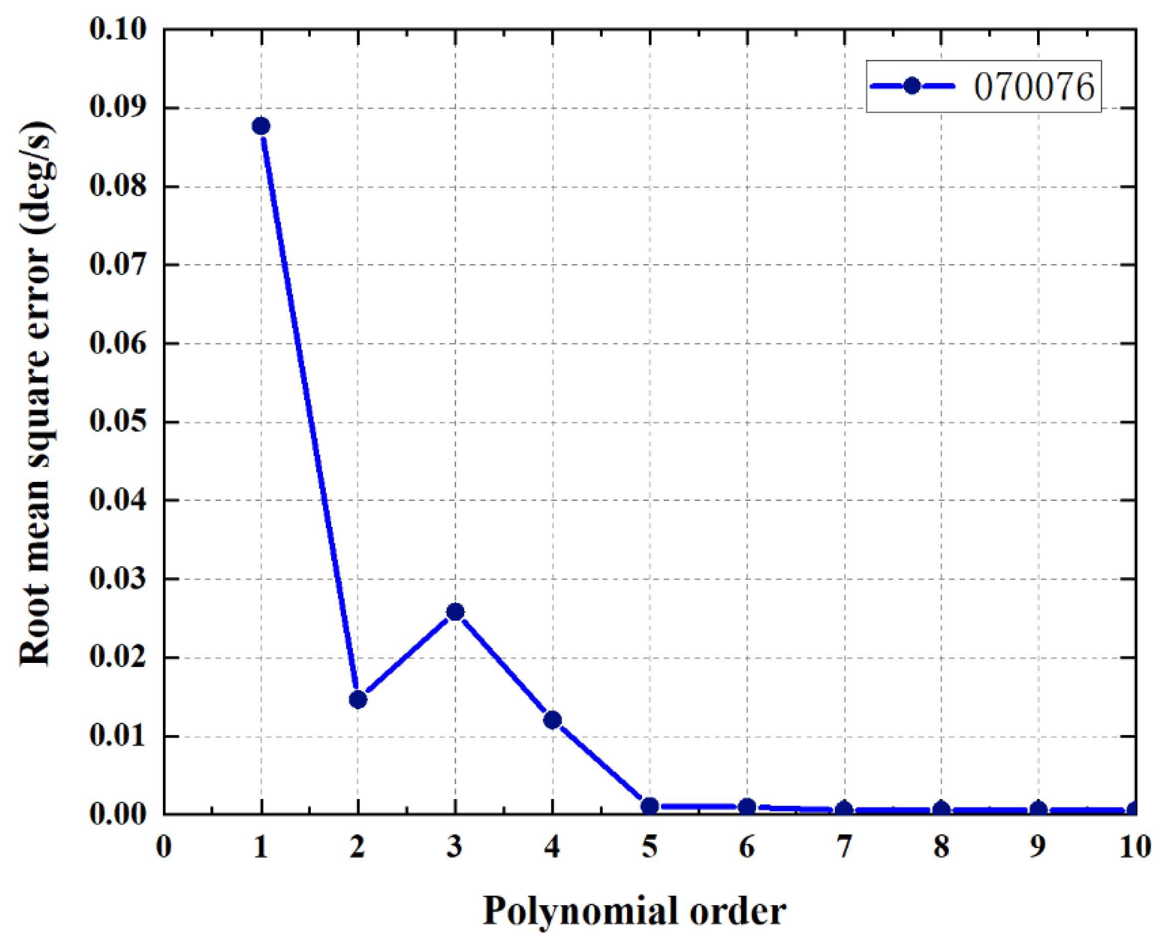
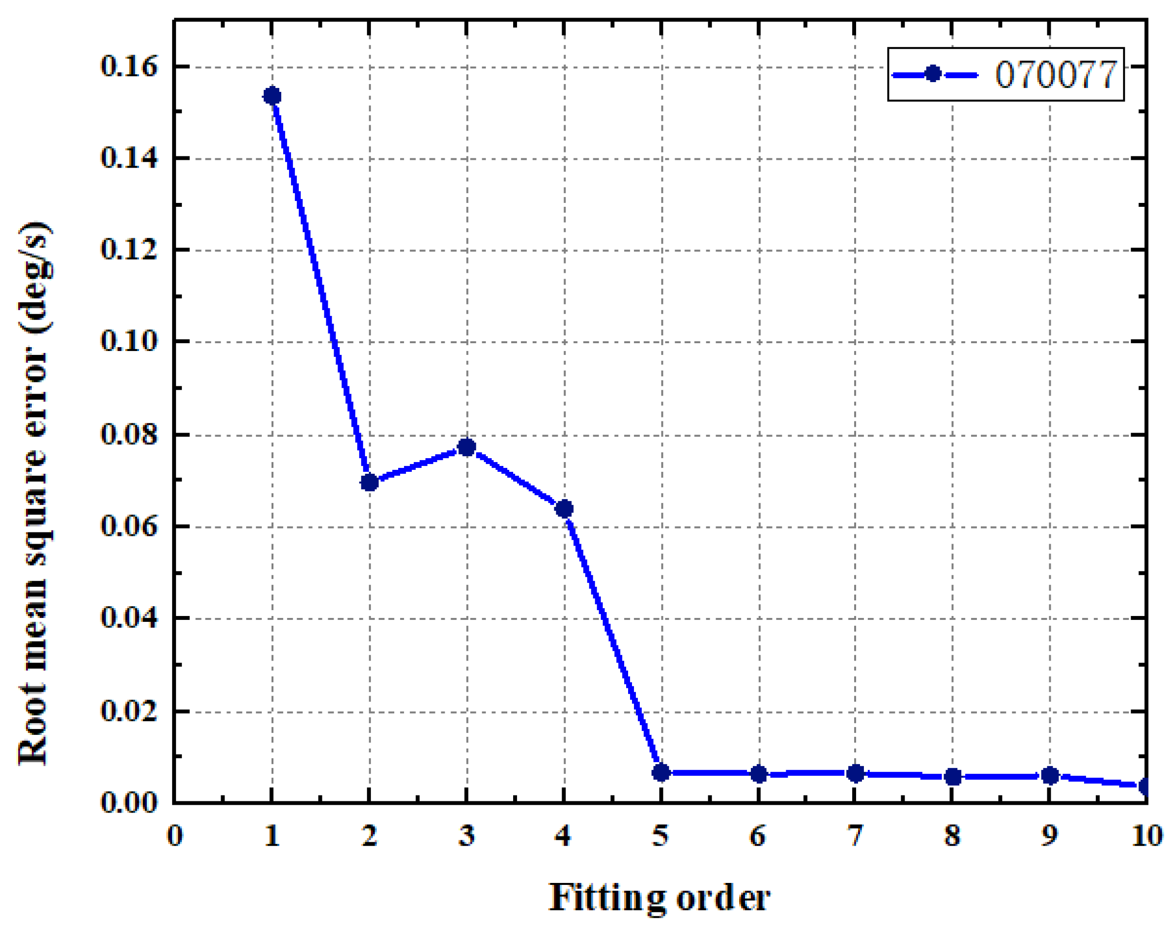
Figure 5 and Figure 6 show the relationship between the polynomial order and RMSE of FOG 070076 and 070077, respectively, on the basis of the data measured at an ambient temperature of 28 °C. The RMSE of the two gyroscopes increased when the polynomial order was 3. However, the error decreased rapidly with an increase in the polynomial order before order 5, and then tended to be stable. For FOG 070076, the RMSE calculated with polynomial order 5 was reduced by 98.74% compared with the results calculated with polynomial order 1. For FOG 070076, the RMSE calculated with polynomial order 5 was reduced by 95.57% compared with the results calculated with polynomial order 1.

Figure 5.
Root-mean-square error vs. polynomial order (070076).

Figure 6.
Root-mean-square error vs. polynomial order (070077).
It can be observed that the TDNP method effectively reduced the fluctuation of the fitting data, even if the order was 2. If the orders exceed 5, the error will continue to decrease, but the amount of calculation will increase, which is not conducive to landslide monitoring. The TDNP with order 5 had a better comprehensive performance.
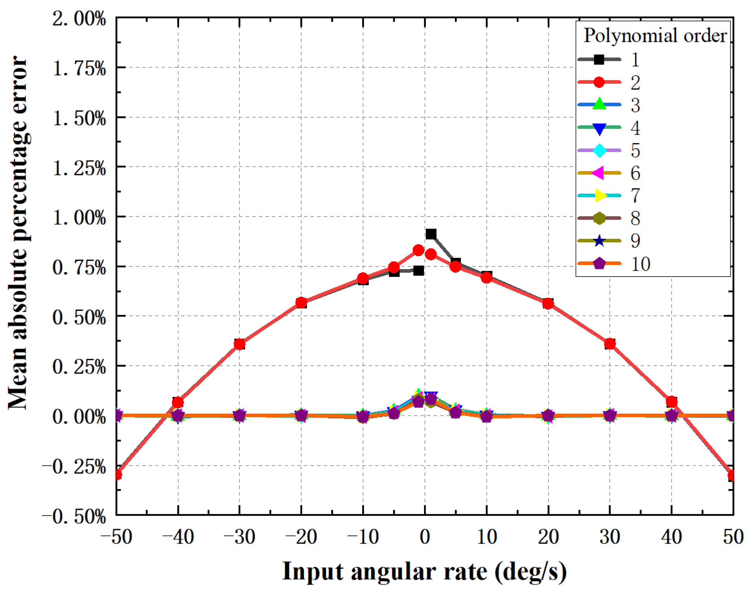
Mean absolute percentage error (MAPE) reflects the reliability of measurements. When a landslide is in the creep stage, the angle of the coupling pipe changes slowly. Consequently, it is necessary to determine the calibration capability of the algorithm for small-angular-rate measurements. Therefore, it is necessary to analyze the MAPE of the measurements when fitting using the TDNP with different orders. The error when the order is n and the angular rate at temperature is is calculated by
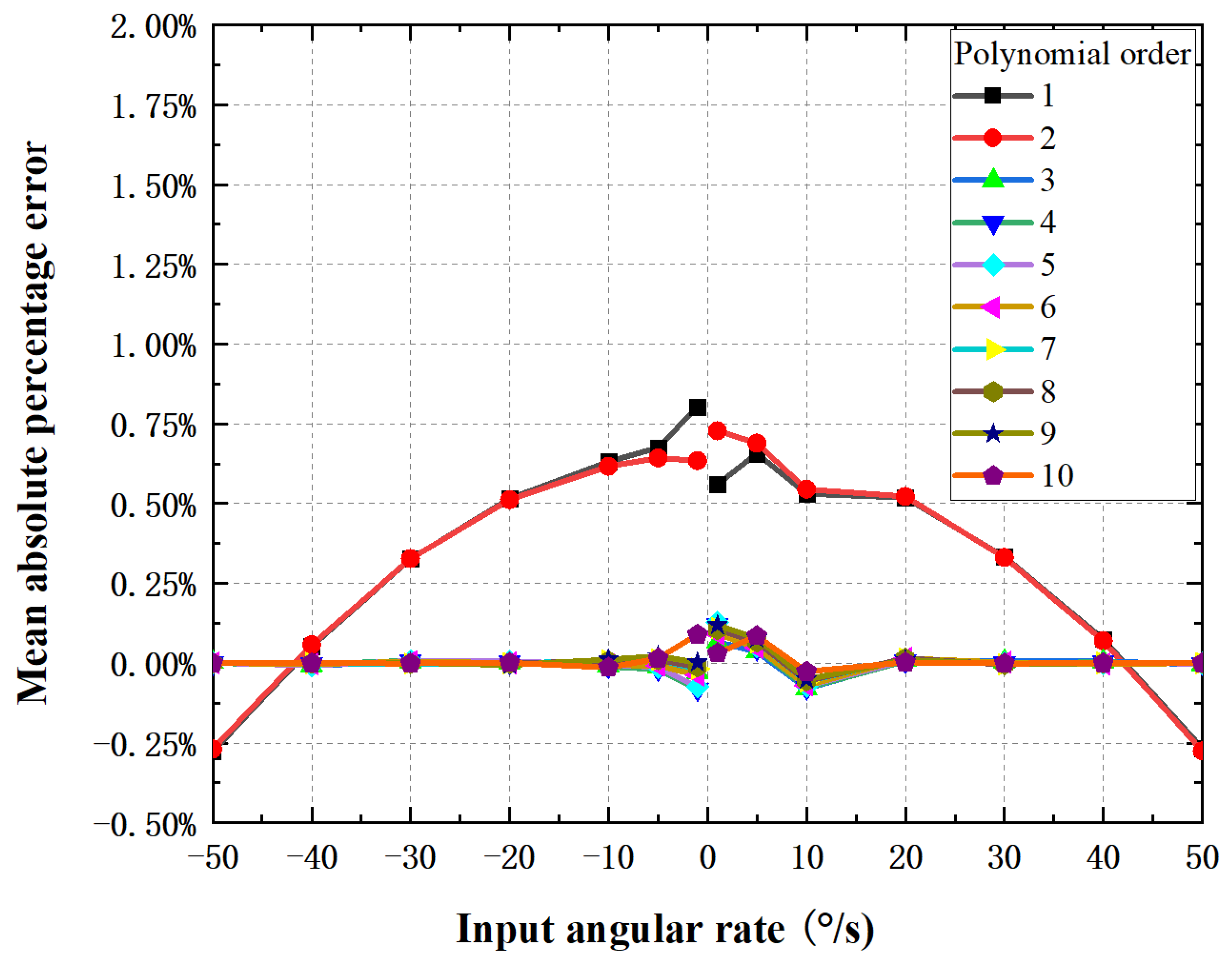
where is the angular rate calculated by the TDNP algorithm with order n at temperature . Figure 7 and Figure 8 present the MAPE curves of FOG 070076 and 070077, respectively. For FOG 070076, when the polynomial order exceeded 2, the MAPE was less than 1‰ in the angular rate range of ±10 deg/s, and when it was away from ±10 deg/s, the MAPE was close to 0. However, for FOG 070077, the negative rate part was similar, but the positive rate part was slightly different. Between 0 and 20 deg/s, the MAPE was less than 1‰, and when it was greater than 20 deg/s, the MAPE was close to 0. When the polynomial order was 1 or 2, the MAPE of the two FOGs was between −3‰ and 9‰, which increased significantly with a decrease in the angular rate.

Figure 7.
Mean absolute percentage error vs. input angular rate (070076).
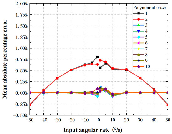
Figure 8.
Mean absolute percentage error vs. input angular rate (070077).
It can be inferred that when a landslide is in the creep stage and the angle of the coupling pipe change is close to 0 deg/s, the reliability of the thermal calibration results is likely to be relatively low, especially when the order of the TDNP is less than 3. However, the reliability is very high when the angle of the coupling pipe change is away from 0 deg/s using the TDNP thermal calibration method, especially when the order of the TDNP is equal to or greater than 3.
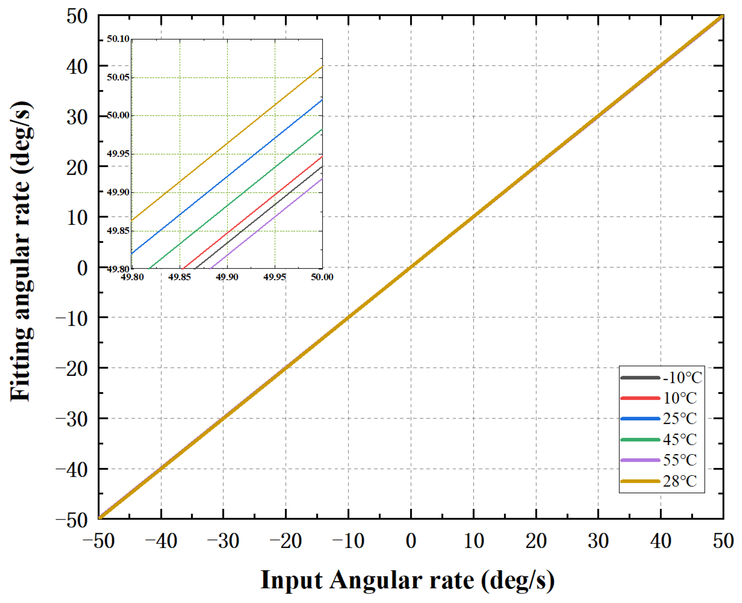
Figure 9 presents the fitting curves drawn on the basis of the TDNP with order 5 at different temperatures. The fitting curves of the two sensors generally exhibited a similar coincidence state. Compared with the standard value, the higher the absolute angular rate, the greater the deviation. Taking 070076 as an example, the drawing of partial enlargement showed that the input and output curves at different temperatures did not completely coincide. When the turntable output the standard rate of 50 deg/s, the measurement error was maximum at −10 °C, 0.06 deg/s, and the smallest appeared around 25 °C, approximately 0.02 deg/s.
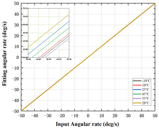
Figure 9.
Fitting angular rate vs. input angular rate (070076).
It can be seen that after thermal calibration, the TDNP method still had risks for landslide monitoring conditions at different temperatures when the angular rate was higher.
4. Thermal Calibration Based on Artificial Neural Network (ANN)
ANN can be trained to approach various linear and nonlinear relationships. Although the ANN thermal calibration method is not suitable for processing measurement data in real time and in situ due to time-consuming, unstable training results and other reasons, the method has reached the accuracy of gyroscopes thermal calibration in some application fields [12,13,14]. Therefore, the ANN method is applied for comparison with the TDNP.
The BPNN is a multilayer feedforward ANN trained according to the error back-propagation algorithm, which adopts the Widrow–Hoff learning algorithm and multilayer network with a nonlinear differentiable transfer function. With continuous in-depth study, many more effective and faster algorithms have been developed. Our group selected the Levenberg–Marquardt (LM), Bayesian regulation (BR), and scaled conjugate gradient (SCG) algorithms to explore the application feasibility of ANN algorithms in landslide monitoring data processing.
The LM algorithm solves the extreme value of a function by iteration, which combines the characteristics of the Newton and gradient methods [21]. It is relatively fast to train a medium-sized feedforward ANN. The SCG is a proportional conjugate gradient algorithm that combines a modular trust region algorithm with a conjugate gradient algorithm to reduce the time required to search the network when adjusting the direction [22]. The SCG algorithm does not require a linear search and requires more iterations than other conjugate gradient algorithms, but the amount of calculation per iteration is smaller; therefore, its calculation cost is lower, and it is very useful in dealing with some large-scale problems [23]. BR is an optimal algorithm for solving the learning problems of ANNs, which can automatically select the regularization parameters and has the characteristics of the high convergence rate of traditional BP neural networks [24].
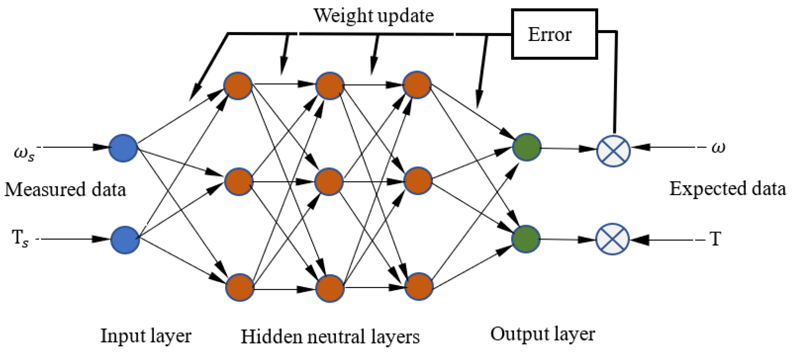
The ANN model was established on the basis of the LM, SCG, and BR algorithms using the same data as in the former TDNP fitting. The structure of the neural network is shown in Figure 10, where is the angular rate measured by the FOG, is the temperature measured by the temperature sensor in the FOG, is the expected angular rate, and T is the expected temperature. A total of 70% of the data were used for training, 15% for practice, and 15% for testing. The number of hidden neuron layers was set from 1 to 18.
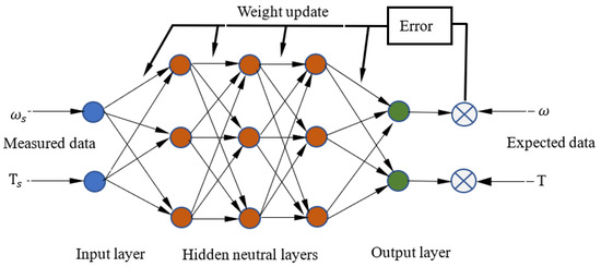
Figure 10.
Structure of the neural network adopted for thermal calibration.
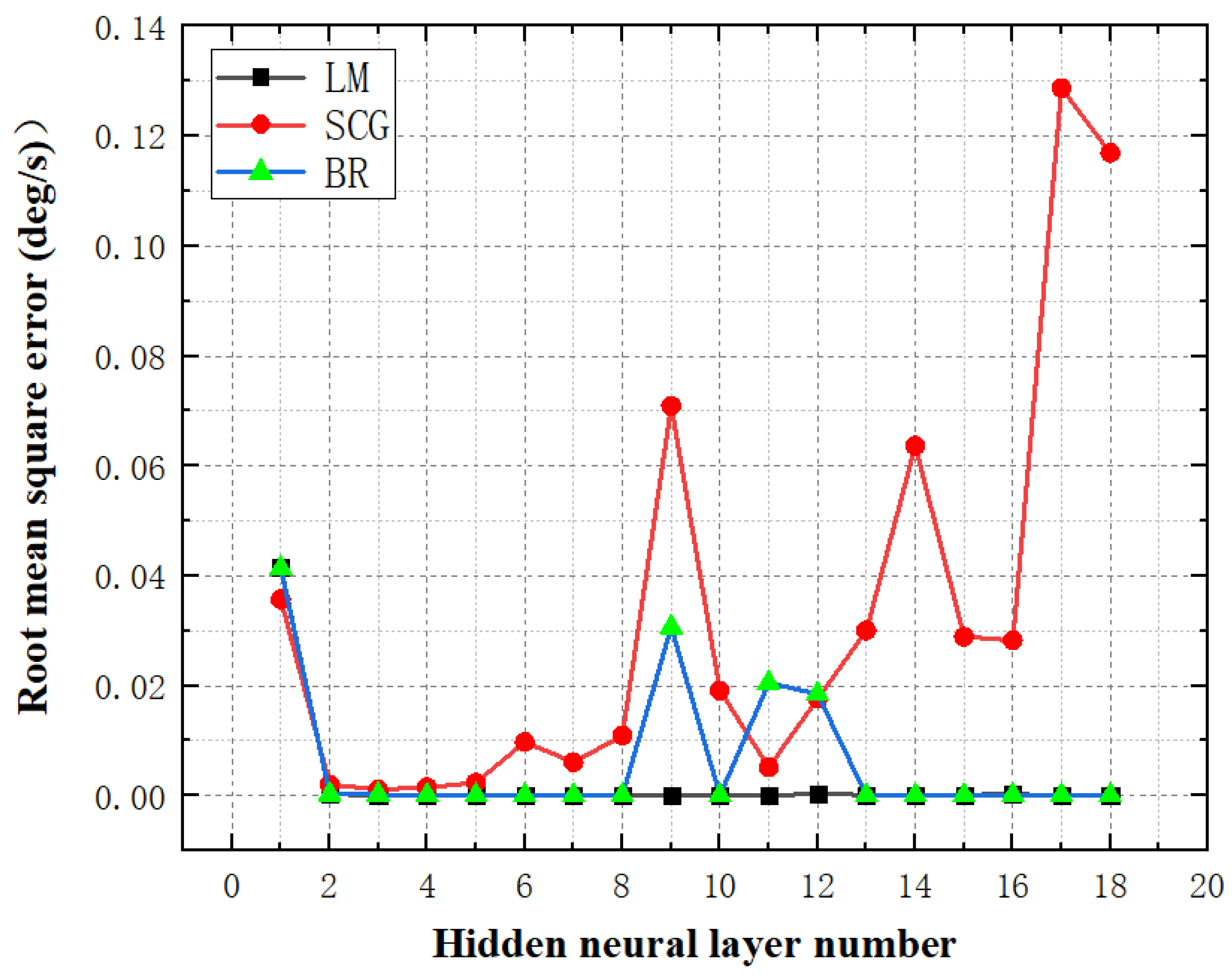
Seventy percent of the data were randomly selected for the training. The actual trainings showed that using the same training method may lead to different results for the same set of data. To obtain a high-quality training network, multiple trainings were carried out, and better data were chosen to calculate the root-mean-square error, as shown in Figure 11 and Figure 12. The root-mean-square error fluctuation using the SCG neutral network was obvious and more unsatisfactory compared to the LM and BR neutral networks. The error using the LM neutral network was slightly smaller and more stable than that of the BR neutral network when the number of hidden neural layers was greater than one. Consequently, the LM neutral network was selected as the final ANN algorithm and compared with the TDNP.
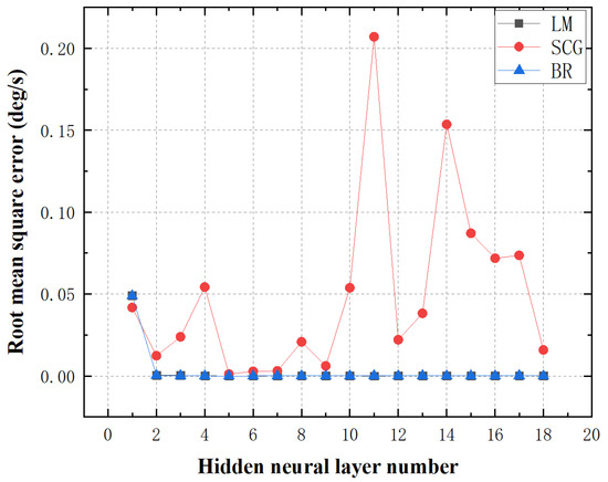
Figure 11.
Root-mean-square error of FOG 070076 (28 °C).
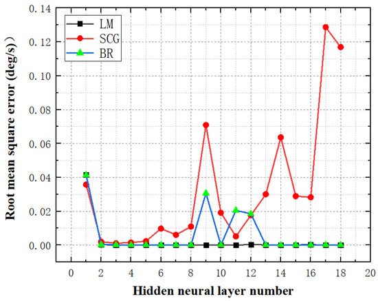
Figure 12.
Root-mean-square of FOG 070077 (28 °C).
5. Discussion of Thermal Calibration Methods and Field Test
5.1. Discussion of Thermal Calibration Methods
Accuracy, speed suitable for in situ and real-time measurement, and stability are the main requirements that determine whether a thermal calibration method is adaptive for landslide displacement measurement. To determine a suitable thermal calibration method for landslide displacement measurement, the mean absolute error was used to compare the thermal calibration capability of the TDNP algorithm with different orders with that of the LM neural network. According to the experimental results shown in Section 3, when the ambient temperature was 28 °C and the order of the TDNP was 2, the RMSE decreased significantly, and the error curve was approximately horizontal when the order exceeded 5. In addition, the smaller the polynomial order, the faster the calculation speed. Therefore, the order of the TDNP was set from 2 to 5. On the basis of the experimental results displayed in Section 4, the LM neural network showed better performance, and the data calculated using the neural network showed that the accuracy was higher when the number of hidden layers was between four and nine. Thus, an LM neural network with five hidden neuron layers and 1000 fitting steps was performed.
Table 1 and Table 2 list the comparison results at the experimental temperatures. The mean absolute error difference between the calibrated and uncalibrated data was not obvious at room temperature, but it was approximately an order of magnitude larger for the TDNP with order 2. Compared with the other methods in the list, the calibration capability of the TDNP with order 2 was inferior, but it had the fastest calculation speed, owing to the minimum amount of calculation. The mean absolute error of data measured by the same kind of gyroscope presented different calibration capabilities for the TDNP with order 3, and gyroscope 070076 was better, especially away from room temperature. The overall calibration effect of the TDNP with order 3 and the LM neural network was similar, and the mean absolute error was reduced by more than 100 times when it was far away from room temperature. When the order was greater than three, the thermal calibration capability of the TDNP was obviously better than that of the ANN. This capability can potentially be improved by using a more advanced ANN. However, the processing speed of the ANN methods is insufficient for realizing real-time and in situ thermal calibration, and the training results are unstable for landslide displacement monitoring.

Table 1.
Mean absolute error of different methods (070076).

Table 2.
Mean absolute error of different methods (070077).
For the entire measuring temperature range, the accuracy of the TDNP with order 5 always satisfied the requirements of landslide displacement measurement on the basis of the assumptions described in Section 1.1.
5.2. Field Test
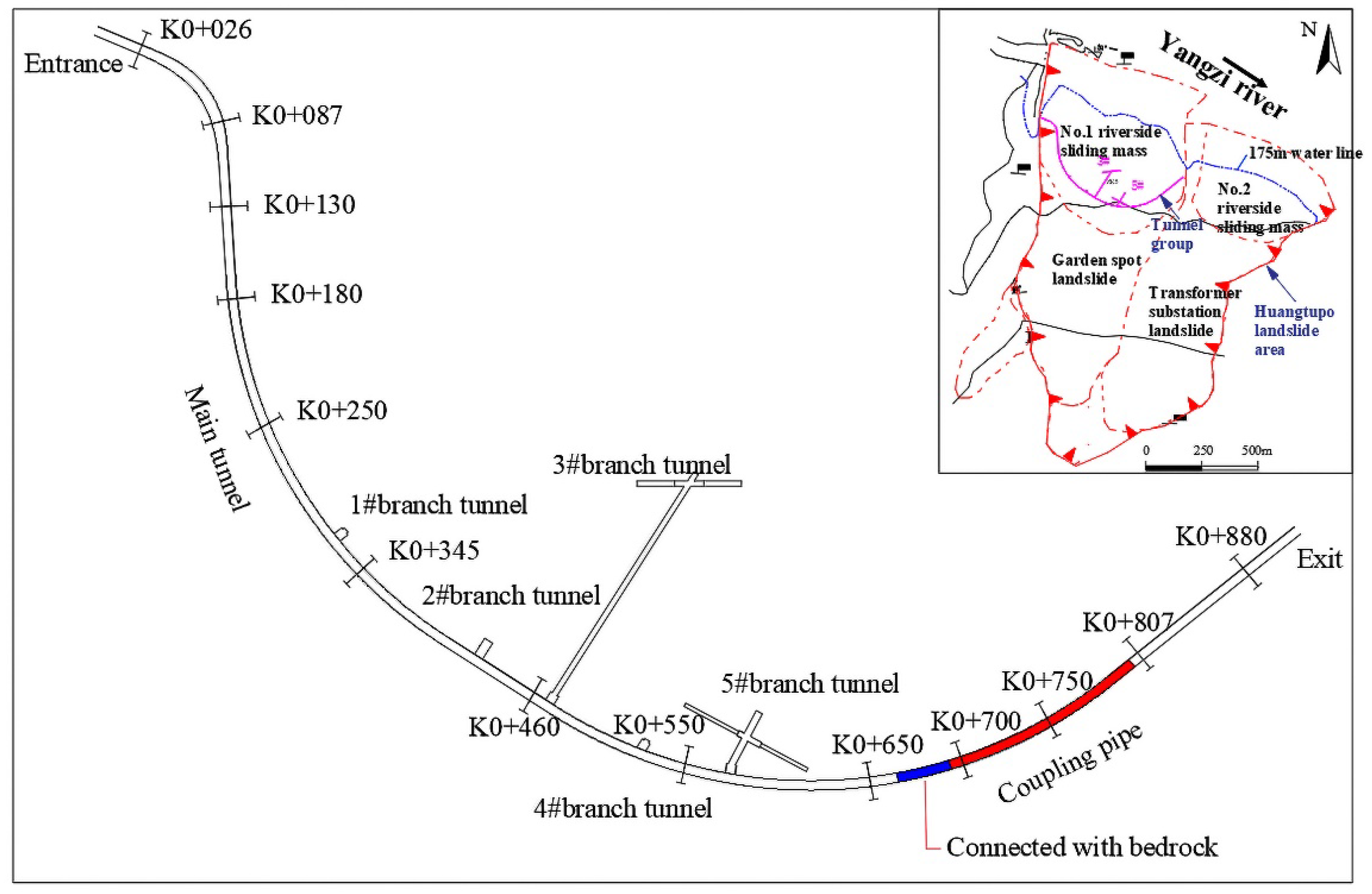
A field test of the TDNP thermal calibration effect was conducted in the tunnel group at the Badong field test site. The Badong field test site is located in the Huangtupo landslide area, one of the largest and most harmful landslides in the Three Gorges Reservoir area of China. Figure 13 shows the internal layout of the tunnel group and the position of the test coupling pipe. Twenty meters of the coupling pipe was fixed to the bedrock, and the remaining 114 m of the coupling pipe was fixed to a sliding mass.
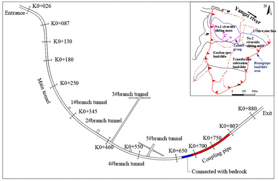
Figure 13.
Tunnel group and the position of coupling pipe.
Figure 14 presents the probe and the PE material coupling pipe with suitable flexibility and rigidity to ensure its capability to be coupled with landslide displacement.
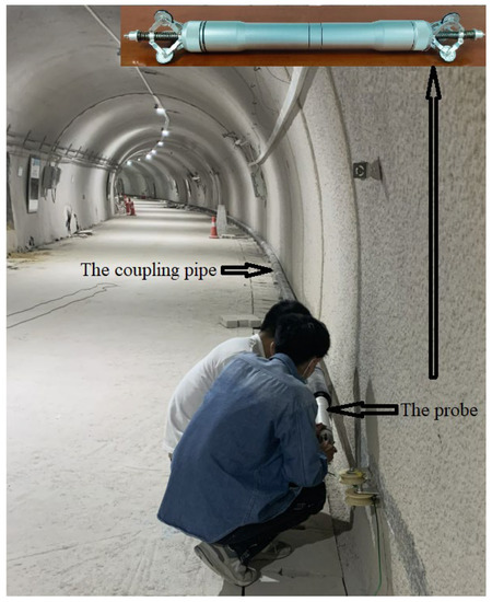
Figure 14.
Field test.
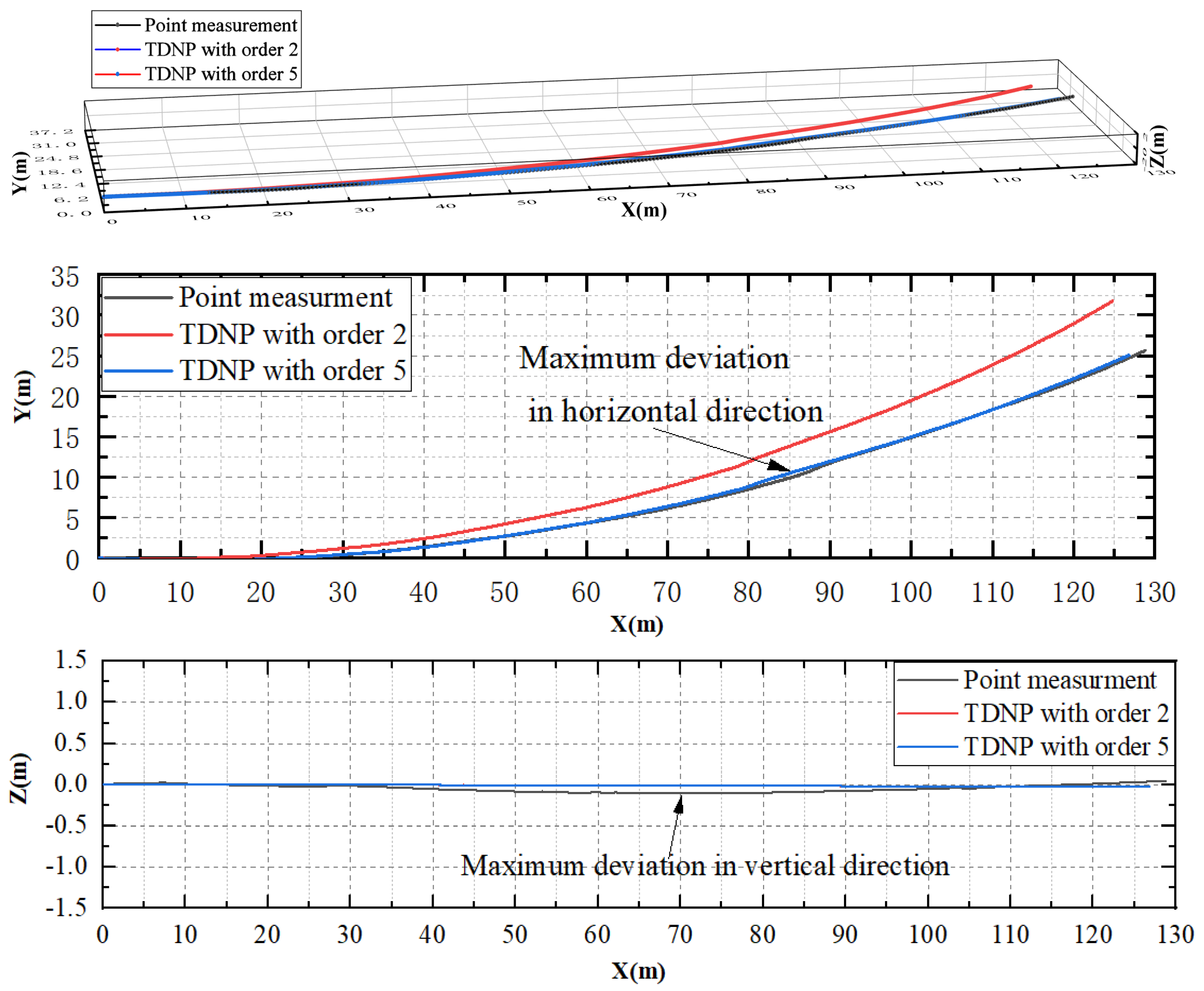
Point measurement is a static measurement method with higher accuracy, but the measurement time is more than two hours per hundred meters. We statically measured the pitch and yaw angle of the coupling pipe at an interval of 0.5 m, and calculated its trajectory, which was taken as the standard trajectory by substituting the mean angle data into the formula of the coupling pipe trajectory. The trajectory of the coupling pipe was also measured by the probe, as described in Section 1.1, whose measurement time was approximately two minutes per hundred meters. TDNP thermal calibration with orders 2 and 5 was carried out for the output data of the gyroscopes that measured the pitch, roll, and yaw angle. Then, combined with the data measured by the inclination sensors in the probe, pitch and yaw angles were calculated after complementary filtering. On the basis of the data of the angles and sample distance, we calculated the coupling pipe trajectories by the same algorithm and compared them with the standard trajectory. Figure 15 presents the field test results that show that compared with TDNP thermal calibration with order 2, the trajectory curve after TDNP thermal calibration with order 5 obviously coincided with the standard one with a higher degree of coincidence and smaller deviation. Comparing the two curves obtained by the TDNP calibration with order 5 and the point measurement method, the horizontal deviation around 85 m in the x-axis direction was larger, up to approximately 50 cm. The coupling pipe was laid smoothly along the tunnel wall, and, thus, the abnormal magnetic field encountered during the point measurement could be the reason for the deviation in this section. The maximum deviation in the vertical direction was 12 cm.
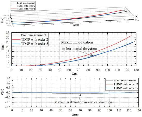
Figure 15.
Field test results.
6. Conclusions
A solution to map the calibration of the FOG thermal drift using the TDNP with different orders is presented. A comparative analysis was performed considering the method of the ANN. First, an experiment that represents the relationship between the FOG output and temperature changes was reported, highlighting that the higher the input angular rate and the farther the deviation from 25 °C, the greater the measurement deviation, with a maximum deviation close to 0.8 deg/s. Then, the thermal calibration processes of TDNP and ANN methods were presented for comparative research. Subsequently, the mean absolute errors of the different methods were listed. The analysis and field test results showed that the method of the TDNP with order 5 had better performance and satisfied the requirements of landslide displacement monitoring for the entire measuring temperature range, when the trajectory angle of a coupling pipe change exceeded one degree within the time interval between two measurements. The detailed conclusions are summarized as follows:
(1) For landslide displacement monitoring, the TDNP method had stable thermal calibration results and higher calculation speed.
(2) When the order of the TDNP was more than three, the thermal calibration capability of the TDNP was better than that of the ANN, as shown in Section 4, especially when the temperature was away from 25 °C.
(3) When the order of the TDNP was equal to or greater than five, there was no obvious difference in thermal calibration accuracy.
(4) The method of the TDNP with order 5 had better comprehensive performance and was adaptive for landslide displacement measurement.
(5) The random thermal drift was reduced by the TDNP method. It is not only applicable to FOG thermal calibration, but also applicable to MEMS and other angular rate sensors with the same thermal drift characteristics.
This research is based on the assumption that the change in the angular rate during the measurement of a coupling pipe trajectory is greater than 0.005 deg/s. If calibrated only by the TDNP method, the angular rate measurement accuracy is unlikely to be sufficient for landslide monitoring when the angular rate is less than that. Comprehensive consideration of various factors and methods could be the way to solve this problem, including analysis of instrument errors, sensor layout optimization, filtering methods, trajectory algorithms, and displacement evaluation methods.
Author Contributions
Data curation, Y.Z. (Yongquan Zhang); funding acquisition, H.T.; methodology, Y.Z. (Yu Zhu); software, H.X.; writing-review & editing, G.L. All authors have read and agreed to the published version of the manuscript.
Funding
This work was supported by the National Natural Science Foundation of China (NSFC) (grant number 41827808, 2019) and the Badong National Observation and Research Station of Geohazards.
Conflicts of Interest
The authors declare no conflict of interest.
References
- Zhang, Y.; Tang, H.; Lu, G.; Wang, Y.; Li, C.; Zhang, J.; An, P.; Shen, P. Design and Testing of Inertial System for Landslide Displacement Distribution Measurement. Sensors 2020, 20, 7154. [Google Scholar] [CrossRef] [PubMed]
- Li, X.; Li, H.; Zhang, Y.; Du, S.; Liu, P.; Yang, H. Cooperation of quadruple cylinder-wound coil and insulation cavities for suppressing the thermal-induced bias drift of FOG. Opt. Commun. 2020, 476, 1–8. [Google Scholar] [CrossRef]
- Kurbatov, A.M.; Kurbatov, R.A. Temperature characteristics of fiber-optic gyroscope sensing coils. J. Commun. Technol. Electron. 2013, 58, 745–752. [Google Scholar] [CrossRef]
- Liu, J.; Liu, Y.; Xu, T. Bias error and its thermal drift due to fiber birefringence in interferometric fiber-optic gyroscopes. Opt. Fiber Technol. 2020, 55, 102138. [Google Scholar] [CrossRef]
- Zhang, B.; Chu, H.; Sun, T.; Guo, L. Thermal calibration of a tri-axial MEMS gyroscope based on Parameter-Interpolation method. Sens. Actuators A Phys. 2017, 261, 103–116. [Google Scholar] [CrossRef]
- Jin, J.; Song, N.; Li, L. Temperature Drift Modeling and Rea-l time Compensation of Interferometric Fiber Optic Gyroscope. Acta Aeronaut. Et Astronaut. Sin. 2007, 28, 1450–1454. [Google Scholar]
- Akimov, P.A.; Matasov, A.I. Estimation of Biases in Gyro Drifts by Means of l1-norm Approximation. IFAC Proc. Vol. 2012, 45, 442–447. [Google Scholar] [CrossRef]
- Gulmammadov, F. Analysis, modeling and compensation of bias drift in MEMS inertial sensors. In Proceedings of the IEEE 2009 4th International Conference on Recent Advances in Space Technologies, Istanbul, Turkey, 11–13 June 2009; pp. 591–596. [Google Scholar] [CrossRef]
- Li, N.; Chen, J.; Yuan, Y.; Han, Y.; Tian, X. Compensation of FOG temperature drift based on LS-SVM modeling. In Proceedings of the IEEE 2016 35th Chinese Control Conference (CCC), Chengdu, China, 27–29 July 2016; pp. 5515–5518. [Google Scholar] [CrossRef]
- Bhatt, D.; Aggarwal, P.; Bhattacharya, P.; Devabhaktuni, V. An enhanced MEMS error modeling approach based on nu-support vector regression. Sensors 2012, 12, 9448–9466. [Google Scholar] [CrossRef] [PubMed]
- Song, R.; Chen, X.; Tang, C. Study on temperature drift modeling and compensation of FOG based on AFSA optimizing LS-SVM. In Proceedings of the 2014 IEEE Chinese Guidance, Navigation and Control Conference, Yantai, China, 8–10 August 2014; pp. 538–542. [Google Scholar] [CrossRef]
- Liu, Y.; Yang, G.; Li, S. Application of BP-AdaBoost model in temperature compensation for fiber optic gyroscope bias. J. Beijing Univ. Aeronaut. Astronaut. 2014, 40, 235–239. [Google Scholar]
- Song, L.; Zhang, W. Temperature error compensation for open-loop fiber optical gyro using back-propagation neural networks with optimal structure. In Proceedings of the 2014 IEEE Chinese Guidance, Navigation and Control Conference, Yantai, China, 8–10 August 2014; pp. 303–308. [Google Scholar] [CrossRef]
- Fontanella, R.; Accardo, D.; Moriello, R.S.L.; Angrisani, L.; de Simone, D. MEMS gyros temperature calibration through artificial neural networks. Sens. Actuators A Phys. 2018, 279, 553–565. [Google Scholar] [CrossRef]
- Wang, W.; Chen, X. Modeling and compensation method of FOG temperature drift based on multi-scale and improved support vector machine. J. Chin. Inert. Technol. 2016, 24, 793–797. [Google Scholar]
- Grigorie, T.L.; Botez, R.M.; Lungu, M.; Edu, R.I.; Obreja, R. Micro-Electromechanical systems gyro performance improvement through bias correction over temperature using an adaptive neural network-trained fuzzy inference system. Proc. Inst. Mech. Eng. Part G J. Aerosp. Eng. 2012, 226, 1121–1138. [Google Scholar] [CrossRef]
- Nez, A.; Fradet, L.; Laguillaumie, P.; Monnet, T.; Lacouture, P. Simple and efficient thermal calibration for MEMS gyroscopes. Med. Eng. Phys. 2018, 55, 60–67. [Google Scholar] [CrossRef] [PubMed]
- Zhu, R.; Zhang, Y.; Bao, Q. A novel intelligent strategy for improving measurement precision of FOG. IEEE Trans. Instrum. Meas. 2000, 49, 1183–1188. [Google Scholar] [CrossRef]
- Secer, G.; Barshan, B. Improvements in deterministic error modeling and calibration of inertial sensors and magnetometers. Sens. Actuators A Phys. 2016, 247, 522–538. [Google Scholar] [CrossRef]
- Niu, X.; Li, Y.; Zhang, H.; Wang, Q.; Ban, Y. Fast thermal calibration of low-grade inertial sensors and inertial measurement units. Sensors 2013, 13, 12192–12217. [Google Scholar] [CrossRef] [PubMed]
- Levenberg, K. A method for the solution of certain non-linear problems in least squares. Q. Appl. 1944, 2, 164–168. [Google Scholar] [CrossRef]
- Møller, M.F. A scaled conjugate gradient algorithm for fast supervised learning. Neural Netw. 1993, 6, 525–533. [Google Scholar] [CrossRef]
- Ribeiro, M.V.; Duque, C.A.; Romano, J.M.T. An interconnected type-1 fuzzy algorithm for impulsive noise cancellation in multicarrier-based power line communication systems. IEEE J. Sel. Areas Commun. 2006, 24, 1364–1376. [Google Scholar] [CrossRef]
- Xu, M.; Zeng, G.M.; Xu, X.Y.; Huang, G.H.; Sun, W.; Jiang, X.Y. Application of Bayesian regularized BP neural network model for analysis of aquatic ecological data—A case study of chlorophyll-a prediction in Nanzui water area of Dongting lake. J. Environ. Sci. 2005, 17, 946–952. [Google Scholar]
Publisher’s Note: MDPI stays neutral with regard to jurisdictional claims in published maps and institutional affiliations. |
© 2022 by the authors. Licensee MDPI, Basel, Switzerland. This article is an open access article distributed under the terms and conditions of the Creative Commons Attribution (CC BY) license (https://creativecommons.org/licenses/by/4.0/).

