Abstract
The design and operation of performant and safe electric vehicles depend on precise knowledge of the behavior of their electrochemical energy storage systems. The performance of the battery management systems often relies on the discrete-time battery models, which can correctly emulate the battery characteristics. Among the available methods, electric circuit-based equations have shown to be especially useful in describing the electrical characteristics of batteries. To overcome the existing drawbacks, such as discrete-time simulations for parameter estimation and the usage of look-up tables, a set of equations has been developed in this study that solely relies on the open-circuit voltage and the internal resistance of a battery. The parameters can be obtained from typical cell datasheets or can be easily extracted via standard measurements. The proposed equations allow for the direct analytical determination of available discharge capacity and the available energy content depending on the discharge current, as well as the Peukert exponent. The fidelity of the proposed system was validated experimentally using 18650 NMC and LFP lithium-ion cells, and the results are in close agreement with the datasheet.
1. Introduction
Electromobility is of paramount importance for the implementation of carbon neutrality targets [1], and its success significantly depends on the performance, safety, and longevity of a vehicle’s electric energy storage system (e.g., battery). Accurate information about the battery’s state at different loads and state-of-charge (SoC) is vital during the design and operation of electric vehicles [2]. In addition to accurate range prediction, precise knowledge about the available battery discharge capacity and energy is necessary for optimizing the performance of the electric vehicle [3] and selecting fuses and other overcurrent protection devices [4]. Thus, there is a need for realistic and efficient battery models that can support simulations [5,6] or onboard control systems [7,8].
Battery models can be divided into three main types: experimental, electrochemical, and electric circuit-based models. Experimental models interpolate the final required data mathematically–based on measurement results on the same physical dimension, which are derived by lengthy laboratory tests when dealing with multi-parametrical systems. First-principle approaches, such as electrochemical models, require a global, in-depth understanding of underlying mechanisms, and in many cases, it is challenging to realize correct model parameters [9]. For example, still, some parameters cannot be measured directly and are usually found indirectly by fitting the model to the results. Electric circuit models, not looking for the reasons, but modeling the electric behavior, proved to be useful [10]: Depending on the complexity of the chosen equivalent circuit, the accuracy of predicting the dynamic behavior of the battery system could be improved without requiring tedious tests under different operating conditions. Moreover, they can easily be adapted and implemented in battery management [11].
Unfortunately, present electric circuit-based methods still suffer from various drawbacks, such as discrete-time simulations of the equivalent circuit must be implemented to precast the battery’s future behavior. For example, to precast the remaining cell energy, many fine-resolved calculation steps need to be performed, leading to a high CPU consumption.
The present paper proposes a set of equations to allow for the analytical determination of the battery characteristics during a constant current discharge, such as the available discharge capacity and the available discharge energy content depending on the discharge current, which is essential for energy system design and operation.
Commonly, the existing electric circuit models parametrize the equation parameters, such as the experimental models based on experiments on the desired physical dimension (e.g., capacity, energy) with the least square of error method (further called “Direct-Fit Method”). Their primary target is, e.g., to interpolate values. The quality of the proposals for equations is judged based on if the shape of the equation can fit with any chosen set of values to the gathered measurement data. While some researchers target the first-principle connection of their parameters, others ignore these explanations completely and focus primarily on modeling the shape.
This research investigates the quality of precast if such a system of equations is not directly fitted to the final results but parametrized by experimenting with the parameters (in this case, internal resistance, open-circuit voltage) independent of the final desired physical dimensions (e.g., constant-current (CC) capacity, energy content). Furthermore, the set of equations was created so that a direct calculation of the final desired values for CC-capacity and CC-energy content without time-discrete steps is possible.
The rest of the paper is organized as follows: The following Section summarizes the previous research studies conducted on battery equations. It also presents the methodological approach and the proposed set of equations to describe cell behavior. The experiments to determine the parameters for an example cell and the experiments with direct measurement to evaluate the precast quality achieved are presented. Section 3 compares the experimental and calculated results. The achieved quality with the new equations is discussed in Section 4. The presented work ends with the conclusions and provides a brief outlook for further work.
2. Materials and Methods
2.1. Previous Empirical Equations
In 1897 W. Peukert empirically derived (1) from measurements with lead–acid batteries [12]. The equation describes the duration of a constant current discharge of the fully charged battery till the clamp voltage reaches the allowed minimum voltage. Different from his original publication, (1) is presented as fixed for the units.
= battery capacity at nominal (1 A) discharge current
= time the battery needs to be completely discharged
k = Peukert exponent
According to Peukert’s empirical equation, a double logarithmic presentation of the discharge time depending on the used current I, will lead to a constant linear slope of . Despite critical discussions in the literature, (1) is still used to compare the performance of new cell types and technologies (e.g., [13,14,15,16]).
Many researchers fit their equations–differently than those investigated in the present research–to the finally needed dimension only (Direct-Fit). The present research compares the new method with three existing empirical equations:
The first equation for comparison is the so-called “Peukert-Bend-Equation” (2) we published in 2017 [13]. It additionally models the behavior observed at high discharge rates: The cells provide less charge than that predicted by Peukert’s Law. That deviation increases with the employed discharge current and leads to a “bend” in the plotted graph. The Peukert-Bend-Equation fixes the units of the classic Peukert equation and models the additional reduction in the available charge at high currents by a multiplied term :
Four constants (, , , ) describe the behavior of a cell type: is equal to the discharge time when using 1 A discharge current, is the classic Peukert exponent, models the shape of the bend in an empirical way while equals the current at which only of the expected (classic Peukert equation) capacity is available. and are fully compatible with the classic Peukert equation. (rate of additional decrease) and (position of the bend) model the reduction at high discharge currents.
The second equation for comparison was published by Galushkin et al. in 2020 [17]. It was called “Generalized Peukert’s Equation” (3). It provides two main advantages compared to the previous equations: First, it fixes the problematic behavior when tiny currents are used (capacity tends to be infinite). Secondly, instead of entirely empirical parameters, which were often used in literature when modifying the classic Peukert equation, all of the parameters have electrochemical meaning.
is the maximum possible capacity at nearly 0 A discharge current. is the current when 50% of the maximum capacity is available ). Exponent n determines the decrease in the cell’s released capacity in the point .
Galushkin et al. [18] identified the disadvantages of the above equation: At very high discharge currents, the voltage at the battery terminals will be lower than the cutoff voltage immediately due to the voltage drop on the internal resistance. Therefore, the battery capacity must be zero at that specific maximum current . This effect was not covered by the equation above and led to the third equation for comparison, the “Modified Peukert’s Equation” (4):
In 2022, Yazvinskaya et al. [19] investigated the last two equations with automotive-grade cells. They state the need to use equations other than the classic Peukert equation when the currents are greater than 2 Cn. The Generalized Peukert’s Equation (3) was applicable up to 10 Cn, and the Modified Peukert’s Equation (4) covered all of the currents.
The parameters of the three empirical equations selected for comparison with the new method are connected with real physical life. For example, the equations are formulated using characteristic currents that can be identified in the graphs. Galushkin et al. chose the current leading to 50% of the maximum charge, which Nebl et al. went for . Nevertheless, all of these parameters describe the final behavior (discharge duration, capacity), not parameters that could be checked separately from the finally desired value.
In all cases—in contrast to the following system of equations—these equations were fitted directly to the results. Even when Galushkin et al. [18] found for the Modified Peukert’s Equation (4) a connection to the basic ECM parameters of a cell, they used the direct end-result fitting procedure for parametrization (experimental values regarding capacity).
2.2. Previous Electric Circuit Equations
The presented work was based on a cell model by Tremblay et al., 2007 [20], which used the SoC as the only state variable and described the battery as a controlled DC voltage source in series with a constant resistance (Figure 1). Tremblay’s equation itself bases greatly on the well-known Shepherd equations from 1965 [21].
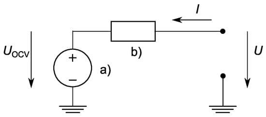
Figure 1.
An equivalent schematic of the electrical characteristics of a lithium-ion battery cell. The schematic representation was composed of (a) a voltage source for the open-circuit voltage in series with (b) the equivalent battery cell internal resistance. The terminal voltage of the battery is indicated with . In the actual case, this system was extended by charge dependent behavior of (a) and charge behavior of (b).
The open-circuit voltage (OCV) of the source was obtained by (5). This equation yields the typical lithium-ion battery OCV curve (see Figure 2), while the constant internal resistance value R was fitted to the measurement data.
= calculated battery terminal voltage (V)
= no-load (open-circuit) voltage (V)
= battery base constant voltage (V)
= polarization voltage (V)
= (virtual) battery capacity (Ah)
= exponential zone voltage amplitude (V)
= inverse exponential zone time constant (Ah)−1
= (constant) internal resistance (Ω)
= = actual extracted battery charge (Ah)
= cell current (A)

Figure 2.
Typical lithium-ion battery open-circuit voltage curve (Example: 2.5 Ah NMC cell; no-load current and in steady-state). Its behavior during discharge contains three phases (right to left): (a) initial exponential decline, (b) in the middle range a slight decrease, and (c) a sharp voltage drop towards its empty state.

The constant value does not describe the increase in the internal resistance when the battery is fully charged (marks at the right axis in Figure 3), although many experiments conducted with lithium-ion cells have clearly shown such behavior [22] (see also Figure 3, lower graph right area). The present paper proposes equations using proper physical units, which include the SoC-dependent behavior of internal resistance.
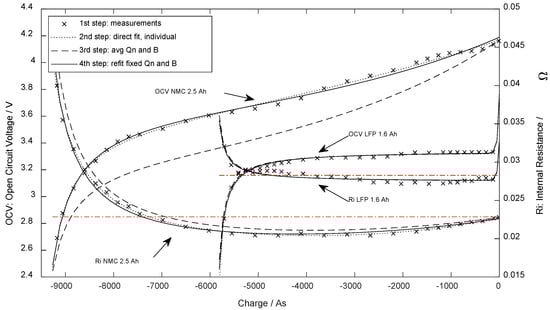
Figure 3.
Open-circuit voltage and internal DC resistance at 25 °C dependent on the extracted charge.
Tremblay et al. stated for [20], as well as their extended version from 2009 [23], that the sets of equations would not model the so-called Peukert effect, which means the discharge current would not change the predicted available capacity under constant current discharge [12]. Nevertheless, the present paper will demonstrate that this kind of equation can well describe the main reasons for the Peukert-effect of lithium-ion cells.
In 2018, Song et al. [14] enhanced the 2007 Tremblay equation [20] with a Peukert-based current-dependent capacity and aging effects. Additionally, they introduced an improved system of equations to parametrize their equations directly from the datasheet. Their research aimed to include capacity degradation, considering temperature, self-discharge, as well as cycling-life but kept the internal resistance parameter independent of the SoC.
2.3. Methodological Approach
Taking advantage of the similarities in the behavior of a cell’s internal resistance to its OCV, the present research proposes a set of electric circuit-based mathematical equations, which are parametrized by only two primary data sources: first, the OCV and, secondly, the internal resistance in relation to the charge. These data are readily available from typical cell datasheets or can alternatively be extracted through a standard measurement procedure (described in Section 2.5). The proposed system thus omits the necessity to store parameters in lookup tables, making it more suitable for efficient simulations. The usage of the proposed system is a compromise between discrete-time application and rough estimations. The proposed equations allow for the direct analytical determination of the Peukert exponent, the available discharge capacity, and the available discharge energy content depending on the discharge current. The proposed method is, therefore, well suited for implementation in the microcontrollers of battery management systems.
Experimental validation of the method was performed for two types of 18650 lithium-ion cells (2.5 Ah NMC as well as 1.6 Ah LFP). The parameterization of the equations via the cell’s internal resistance and OCV curves was demonstrated, as well as the parameter extraction out of discrete-time measurement data. The system does not need fitting against the discharge duration or other final results, as it is entirely based on the OCV and internal resistance parameters. Finally, the experimental results of available charge, energy content, and the Peukert exponent during constant current discharges are compared to predicted values from the proposed equation system.
2.3.1. The Proposed Mathematical Equations
Equation (5) has been widely discussed in the literature. It adequately describes the OCV discharge characteristics of various lithium-ion cell types (e.g., LMO, NMC, LFP) [24,25]. In Tremblay 2007 [20], the internal resistance is presented by a mean value for all operating conditions ignoring changes over charge.
Nevertheless, laboratory experiments performed for that research showed that (5) can also be successfully applied to describe the shape of the SoC-dependent behavior of the internal resistance. Furthermore, the presented system of the equations benefited from the resemblance of the parameters and for the OCV and internal resistance.
As shown in Figure 1, the current was defined in the opposite direction to allow the integration of positive currents to calculate the battery capacity, as in (8). This leads to different signs in the first fundamental Equation (7) compared to (5), where is negative for discharge currents and positive for charge currents.
= (virtual) battery capacity of voltage fit (As)
= exponential zone voltage amplitude (V)
= inverse exponential zone constant of voltage fit (As)−1
= = actual (extracted) battery charge (As)
The zero point for capacity determination, according to (8), was set after a full constant current-constant voltage charge to . As a result of these two decisions, the values for are negative under normal operating conditions, as shown on the abscissa in Figure 2.
Equivalent to (6), the voltage drop on the internal resistance must be considered for calculating the terminal voltage :
= internal resistance (Ω)
Comparing (7) with the experimental data for NMC as well as LFP cells, it could be shown that the shape of (7)—intended for voltage—also covers the internal resistance behavior of lithium-ion cells (compare marks in Figure 3 with the solid line) leading to the second fundamental equation, (10):
= base resistance (Ω)
= polarization resistance (Ω)
= (virtual) battery capacity of resistance fit (As)
= exponential zone resistance amplitude (Ω)
= inverse exponential zone constant of resistance fit (As)−1
Comparing the experimental data and taking into account a common mechanistic/electrochemical background for greater changes of and , it was concluded that the characteristic parameters for the bend positions should be similar regarding and . This allows for reducing the complexity of the equations by merging these parameters using the average value of both fits after the fitting process, refer to (11) and (12). The proposed method for fitting the base parameters is discussed in Section 2.5, and the results are shown in Figure 3.
Combining (4)–(6) with (11) and (12) led to the final Equation (13), which can be parametrized fully by direct measurements.
The maximum cell voltage at = 0 As (100% SoC) and = 0 A is given by:
2.3.2. Assumptions and Limitations
The proposed system in (13) is based on several assumptions. First, the internal resistance does not shrink with the rising amplitude of the current. Secondly, the equations target to describe the discharge process only. Thus, the fact that the cell parameters might not be similar for the discharging and charging currents was ignored. Third, the self-discharge (practically irrelevant for the present research) and aging of the battery (reducing both cell charge and energy) are not available, and over-discharge ( < and esp. <) or overcharge conditions ( > 0 As) are not considered. Additionally, the temperature effects (environmental/starting temperature as well as the rise of temperature while discharge) are not included.
2.3.3. Determining the Maximal Usable Cell Capacity
In the following part, the derived equations are used for the direct calculation of the target cell parameters (such as available energy content and charge content) without the need for direct experiments regarding these parameters.
It is essential to mention that parameter is not the maximal usable capacity , even for infinite small currents, as it includes the charge drawn till 0 V, instead of stopping the discharge at . The maximal usable capacity for very small currents could be obtained by setting (13) equal to , which will yield (15):
The equation cannot be entirely solved for . To use it anyway, an approximately correct value of can be used as with typical lithium-ion cells, the exponential zone (refer Figure 2) has very little influence on the empty cell voltage, resulting in . Thus, can be replaced by without lowering the quality (<0.04%).
2.3.4. Mathematical Charge Content Estimation
The available discharge capacity of a battery or any other energy storage can be determined by integrating the current of a full discharge procedure of a fully charged (CC-CV for lithium-ion cells) cell to the minimum allowed voltage at .
I = applied constant discharge current (A)
For different discharge currents, the available charge varies, leading to a dependency of the discharge duration on the applied discharge current when the discharge is conducted until the cut-off voltage of the cell (Peukert behavior [12]). Thus, the usability of the equations at constant current discharge was investigated. As the charge behaves linearly in time at constant current, (16) was simplified to (18), with the discharge current starting at t = 0 s.
Taking (13) into account and simplification leads to (19):
It is not possible to solve (17) with (19) for . Instead, the resulting discharge duration, depending on an approximated discharge duration , was expressed by the recursive Equation (20).
In some circumstances, it is necessary to avoid recursive calls, e.g., to reduce CPU load. The moment of break-off is dominated by the sharp voltage drop towards the cells empty state, especially for lower discharge currents. Additionally, the parameters contribute little in comparison to the other terms. Moreover, adds time while reduces the discharge time. Thus, dependent on the purpose of usage of the equation system, this part may, therefore, be ignored. Doing so is strongly simplifying (20) to (21), which allows for directly calculating the respective discharge time for each current:
To reduce the error, it is recommended to replace . This reflects that with most currents, approximately the ideal capacity can be used. It turns (20) into (22). That assumption can nearly remove the error caused by non-iterative usage for lower and normal currents completely and also improves the results for very high currents.
Figure 4 presents a comparison of the predicted results between the differently simplified mathematical equations.
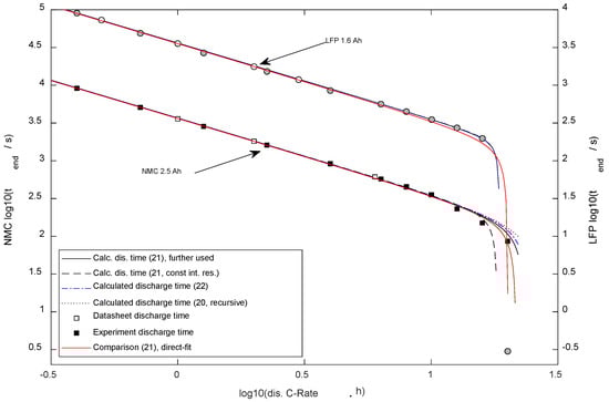
Figure 4.
Discharge duration dependent on the discharge current (the typical Peukert plot). Two y-axes were used to avoid overlay of NMC and LFP results.
First, (20) was calculated iterative (five times); the result is shown in Figure 4 as a dotted line. Secondly, (21), presented as a solid line, showed a Standard error vs. (20) of 34 s with the NMC-cell and 0 s regarding the LFP-cell. Thirdly, (21) was employed in a simplified way, with the usage of the constant SoC-independent (average) internal resistance value, and it is presented as a dashed line. The minimal deviation was found for smaller currents, whereas using the equation with constant internal resistance predicted immediate switch-off for the NMC cell at maximum current (20 Cn), whereas, in reality, a discharge was possible (Cn is the nominal battery capacity divided by 1 h). For the LFP cell, the standard error vs. (20) was 2 s. Finally, (22) was calculated and presented as a dash-dotted line. Standard error vs. (20): 6 s with NMC, 0 s for LFP.
Comparing the different proposals to calculate the discharge time with two different types of lithium-ion cells, it can be seen that the errors between the forecast and experimental results were far higher than the errors caused by the simplification of calculation. For the LFP cell, the results of the proposed equations differed little as of the very narrow exponentiation zone. Thus, it is recommended to calculate , which is a parameter for the following equations, using (21), the simplest equation supporting high currents for the NMC cell type. The first singularity (i.e., the pole) needs to be considered as the maximal possible current (immediate break-off) in any version of the equation; higher currents lead to an immediate break-off ().
2.3.5. Relation to Peukert’s Exponent
The classic Peukert equation (1) leads to a straight-line representation (negative linear slope ) when plotting the employed constant current I versus the reached discharge time , and both axes are scaled in a logarithmic order. The experiments and application of the proposed equations using (20)–(22) with the exemplary specimen showed its validity for reflecting the Peukert behavior up to discharge C-rates of approximately 5 Cn (see Figure 4 and Figure 5), in which the Peukert exponent can be derived from (23).
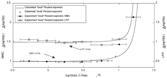
Figure 5.
“local” mean Peukert exponents, which are valid for a specific span of discharge current as presented by the bars.
The limits of the Peukert Equation were clearly visible in the experimental results in Figure 4, as the exponent showed to be dependent on the discharge current. For comparison, calculated “local” values for k following (24) were compared with the experimental values as well as the values derived from the cell’s datasheets in Figure 5.
For the determination of a single characteristic Peukert exponent, the engineer needs to define two certain currents. Usage of the discharge currents according to C-rates of 0.5 Cn and 5 Cn with (23) and (22) is proposed for comparing lithium-ion cells, as the cells showed stable values for that range.
2.3.6. Mathematical Energy Content Estimation
The average discharge voltage may be calculated by integrating the terminal voltage over time during discharge with the discharge procedure starting with a full cell and stopping at . Equations (25) and (26) represent the time-weighted average discharge voltage .
During the constant current discharge, the available energy content depends on the respective discharge current, and that can be readily obtained from , using (21) and (26), which leads to (27).
2.3.7. Comparison with Direct-Fit Method
Many researchers fit their equations—differently than those investigated in the present research—to the finally needed dimension only. Their primary target is, e.g., to interpolate values. In the last step, the proposed method (to experimentally gain the primary factors of internal resistance and open-circuit voltage to precast the finally needed dimension) was compared to the results of that method.
First, the research investigates the overall potential of the shape of the equation to meet the experimental values. Two goodness of fit were compared statistically: (a) the equation on discharge duration fitted to meet the validation samples (direct-fit), and (b) usage of the same equation but parametrized by collecting the ground laying parameters.
Secondly, the proposed equation on constant-current discharge capacity (in both ways of parametrization) was compared to three equations based on the literature using the direct-fit method.
2.4. Experiments
Experimental validation of the method was performed for two types of 18650 lithium-ion cells. These specimens and the used laboratory equipment are presented in the following subsection.
2.4.1. Devices
Before and between all tests, the specimens were kept at 25 °C in a VT4011 temperature chamber for at least one day. The VT4011 temperature chamber provides ±0.5 K accuracy [26].
Due to the high laboratory load (shortage of free devices) and to cover the wide current range, different electric sources/sinks had to be used.
The Zahner Zennium electrochemical workstation PP241 has one channel with ±40 A in the voltage range ±5 V. It provides a voltage accuracy of ±0.1% relative to the value ±1 mV and a current accuracy of ±0.25% relative to the value ±1 mA [27].
The Array 3721A is a 400 W DC load (up to 40 A). It provides a current accuracy of ±0.1% relative to the value ±10 mA and a voltage accuracy of ±0.1% relative to the value ±10 mV [28].
The Bitrode MCV4-100-5 CE battery cell tester provides ±100 A (0 V to 5 V). The voltage and current measurement accuracies are ±0.1 A/±5 mV [29].
The Neware CT-4008-5V6A-S1 cell battery tester has eight channels with ±6 A in the voltage range ±5 V. It provides a voltage accuracy of ±2.5 mV and current accuracy of ±3 mA [30].
The Kelvin connection for connecting the specimens to the devices ensured that contact and lead resistances did not influence the measurements.
All of the employed devices provided time resolution better or equal to 100 ms. The measurement errors dependent on the equipment used were calculated for all of the individual data points. The analyses led to an overall maximum charge error of 81 As, a maximum average discharge voltage error of 13 mV, and a maximum energy error of 284 Ws (for most data points, the calculated error was far more minor). The measurement errors caused by the equipment were generally smaller than the deviations compared in the study, so the measurement errors were not individually detailed in the results presented.
2.4.2. Specimen
First, a 2.5 Ah lithium nickel manganese cobalt oxide (NMC) cell INR18650-25R from Samsung SDI was selected as its available datasheet [31] contained test results, which helped to evaluate the quality. According to the datasheet, the minimal cell voltage is 2.50 V and the maximum cell voltage is 4.20 V.
Secondly, to be able to check the equations with cells of differing OCV-SoC behavior, a second cell type, a 1.6 Ah lithium iron phosphate (LFP) cell HTCFR18650 from Goldencell ( 2.50 V, 3.65 V), was chosen. The according datasheet [32] contained the test results in the current range up to 3 Cn.
Lithium-ion cells change their parameters when they are in use. These changes are great when the cells are new [33]. For steadier cell parameters during the performed tests (SEI layer stabilization), all of the specimens were cycled prior to the tests using CC (constant current) discharging with 0.8 Cn to 2.50 V and CC charging with 0.4 Cn to 4.20 V (NMC)/3.65 V (LFP). Every cell was cycled five times, including a final constant voltage (CV) charging phase, until the current dropped below 0.04 Cn.
After cycling, all of the specimens were statistically investigated to identify the non-representative cells. During these pre-tests, the temperature of the cells and the environment was kept constant at 25 °C. The investigations first encompassed a capacity determination (CC/CV, 1 Cn, down to 0.001 Cn) and, secondly, an open-circuit voltage and internal resistance measurement at 90% SoC. After that, all of the cells were CC/CV charged (0.4 Cn, down to 0.001 Cn) to ensure equally charged cells for further tests. Capacity deviations from the average below 1.5% were deemed acceptable for the following tests.
2.5. Experiments for Parameter Determination
As the fidelity of the proposed system of the equations significantly depends on the accurate determination of the basic parameters, the details of the performed tests are given here.
2.5.1. Determination of the Internal Resistance and Open-Circuit Voltage as a Function of the State of Charge
The equations based on the open-circuit voltage and internal resistance depending on the charge were obtained from a single fully automated measurement using the following procedure on the Bitrode MCV4-100-5 CE cell tester [29].
With the fully CC/CV-charged specimen, the following step was repeated until the minimum voltage was reached: First, after one hour of waiting without current (according to Keil and Jossen [34], a period long enough for stable results at room temperature, sample rate: 1 sample per minute), the measurement rate was increased to 10 Hz. Secondly, a discharge pulse of 1.6 Cn was imposed for 300 ms. Thirdly, the SoC was reduced to the next desired charge level with 0.2 Cn. The desired steps were 5% SoC, but 2.5% in the ranges >80% and <20% SoC. Finally, the measurement rate was again reduced to 1 sample per minute, and the next 1 h waiting phase was started. The Bitrode cell tester guarantees the absence of any current flow during the rest phases.
The whole process took about 70 h. The current pulses were performed in the positive direction when the SoC was smaller than 25% to avoid early undervoltage break-offs from the current discharge pulses at low SoC. The influence of this approach on the gained result for the internal resistance was validated with a second cell of the same type and caused below 5% deviation. Finally, a PHP [35] script scanned the discrete-time data for the high current steps. To find the open-circuit voltage and the average voltage of the last three minutes before the slope was taken into account. The internal resistance was determined by the Δ U/Δ I method [36], using the last value before the slope and the first recording during the pulse (Δ t = 0.1 s). The results are shown in Figure 3 (marks).
2.5.2. Fitting Method to Parametrize Equations
To extract the parameters from the experimental data, a three-step approach was used: in the first step, the least squares approximation method was used for the open-circuit voltage and internal resistance individually (dotted line in Figure 3). Secondly, the parameters and were obtained using (11) and (12), which caused a global deviation of the parameters (dashed line in Figure 3). In the last step, the rest of the parameters were optimized by refitting them against the experimental results while and were forced unchanged (solid line in Figure 3). The parameters found through the test are stated in Section 3.1.
2.6. Experiments for Validation: Recording Real Cell Behavior during Full Discharge Procedures
These experiments were performed to accumulate comparative data to evaluate the proposed equations. The experimental results were used in addition to the given results from the datasheet (Figure 4, Figure 5, Figure 6 and Figure 7).
A uniform distributed temperature change is necessary to avoid regional temperature gradients in the specimen during testing. As the heat conduction within the cell is limited, all of the discharge tests were conducted in a thermally isolated environment to ensure equally distributed temperature changes in the specimen for all tests, in particular for the high current tests. The cells were wrapped in a piece of non-flammable glass wool to reduce heat exchange to the environment. That approach somewhat fits the cells’ behavior in bigger packs of cylindrical cells without a cooling system. In these arrangements, the cells in the center are isolated from the environment and have a similar temperature slope to their neighbors. The pre-temperaturized specimen was placed in that arrangement just before the final tests were started. After removing 7% of its capacity, the cell was recharged to ensure equivalent conditions for all of the compared cells and currents. After the constant voltage phase, the specimen lost not more than 1.0 °C of temperature. Now, the specimens were discharged with the respective test current until the minimum voltage was reached. The employed C-rates for both cells were calculated following (28). The recording rate was 1 Hz. Only cells, which were used below 3 Cn, were used after a capacity check for other (current) tests again.
3. Results
In this section, the first step is to investigate how the good values gained by the parametrized SoC-depending Equation (7) for OCV and (10) for internal resistance-correspond with the directly collected experimental data points regarding these primary parameters (OCV, internal resistance). In the second step, the quality of the precast based on the equations (discharge capacity, voltage, and energy) using these parameters is validated.
To do so, the two following statistical methods were employed:
Relative maximum approximation errors between the predicted values based on the parametrized equations and the results of the validation experiments were calculated to describe the most significant deviation, as is shown in (29).
The standard error between the predicted values and the experimental results was determined to describe the overall quality of the approximation. It was calculated following (30), with degrees of freedom for the initial fitting of OCV and internal resistance parameters (Figure 3), to check the quality of the parametrized equations and with for the comparison with the free fitting of the discharge duration (21) to the final samples.
As some of the calculated graphs based on the equations did not deliver a valid value for the maximal validation current point (e.g., (21) for currents bigger than the mathematical pole when ), this experimental point had to be excluded from the statistics to allow for a direct comparison of all variants.
3.1. Parametrization
Figure 3 presents the OCV curve and the DC internal resistance determined for one of the specimens (marks). The dotted line shows the first direct fitting result of (7) and (10). The deviating dashed line is the result after aligning and according to (11) and (12). For the LFP cell, the parameters deviated little, while the deviation before alignment was far higher for the NMC cell. The final and further used parameters after refitting are presented as a solid line.
The found and further used parameters are presented in Table 1.

Table 1.
Fitted and further used parameters on open-circuit voltage and internal resistance.
The derived parameters for the 2.5 Ah NMC cell were:
= −9257 As = −2.57 Ah~−95%
Peukert’s exponent = 1.037 ( vs. )
The derived parameters for the 1.6 Ah LFP cell were:
= −5803 As = −1.61 Ah~−98%
Peukert’s exponent = 1.013 ( vs. )
Using the eight parameters above and comparing Equations (7) and (10) with the parametrization measurement results (Figure 3), the standard error for the OCV fit was 25.4 mV ( = 0.9%) for NMC specimen and 15.2 mV ( = 1.2%) for LFP. The standard error (DF = 5) for internal resistance was 0.375 mΩ ( = 2.9%) for the NMC cell type and 0.406 mΩ ( = 2.5%) for LFP.
Additionally, the average internal resistance was calculated (weighted equidistant on SoC) to validate if the terms regarding the DC internal resistance depend upon the SoC (In this comparison, when using , and were set to zero). These values are presented for comparison in Figure 3 as horizontal lines and in the last row of Table 1.
3.2. Discharge Duration
Figure 4 presents the calculated discharge time dependent on the discharge currents based on the parametrized equation. For comparison, the experimental results ( Section 2.6) and datasheet references are plotted in Figure 4.
With the LFP cell, the highest current (32.1 A) of the validation experiment led to an immediate (0.3 s) break-off. The system of equations (Figure 4) well forecasted that behavior.
Comparing results of (21) with the experimental data, the standard error (DF = 0) for the NMC cells was 217 s ( = 23%) and for LFP was 141 s ( = 8%).
3.3. Local Peukert Exponent
The local valid Peukert exponent was derived from the experimental and datasheet data. These values and the exponent calculated by Equation (24) are displayed in Figure 5.
Experimental as well as datasheet data in the low current range of both cells resulted in exponents below 1. This was not surprising, as higher currents lead to a temperature rise, which reduces the internal resistance [16].
3.4. Charge
Figure 6 shows the available charge content of the cells depending on the used discharge current read from the datasheet and own experimental data, compared to the calculated data.

Figure 6.
Available Charge dependent on the discharge current.
Figure 6.
Available Charge dependent on the discharge current.

The standard error (DF = 0) regarding the NMC cell was 534 As ( = 23%) and regarding the LFP cell 194 As ( = 7%). As the calculation of the charge is directly based on the discharge time, -statistics were similar.
3.5. Average Voltage while Discharge
During the discharge procedures of the validation tests, the voltage was recorded every second. Figure 7 presents these validated average voltages compared to the calculated data according to (26).

Figure 7.
Average voltage dependent on the discharge current.
Figure 7.
Average voltage dependent on the discharge current.

The standard error (DF = 0) regarding the NMC cell was 36 mV ( = 1%) and regarding LFP it was 69 mV ( = 3%).
3.6. Usable Energy while Discharge
Based on the average voltage and available charge, the usable energy was determined. Figure 8 compares the validated available discharge energy with the predicted data based on (27).
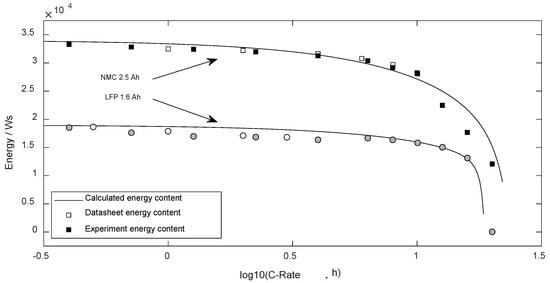
Figure 8.
Energy content dependent on the discharge current.
The standard error (DF = 0) regarding the NMC cell was 1610 Ws ( = 23%) and regarding LFP 995 Ws (= 10%).
3.7. Comparison with Direct-Fit Method
The following subsection compares the proposed method (parametrization by investigating the ground-laying parameters, in this case: internal resistance and open-circuit voltage) with the commonly employed way (fitting to samples of the final desired physical dimension, direct-fit method, in this case: discharge duration and available charge).
3.7.1. Discharge Duration
As a first step, the overall potential of the shape of Equation (21) to describe the discharge duration was investigated using the Direct-Fit Method and compared statistically with the proposed method. To do so, the five parameters , , , , and of (21) were fitted without any constraints to meet the experimental results best.
A simplex downhill algorithm minimized the mean square error (usage of MATLAB fminsearch-function). To allow for comparison under a standard environment, the fitting was performed without any modified fitting options. The values presented in Table 1 were used as the starting parameters. The fitting result is shown in Figure 4 for comparison. The free fitting directly to the final dimension lead for the NMC cell to a standard error (DF = 5) of 249 s ( = 20%) and for the LFP cell of 125 s ( = 14%), while the standard error using the proposed method (DF = 0) was 217 s ( = 23%) for the NMC cell and for the LFP cell 141 s ( = 8%).
3.7.2. Equations from Literature Regarding Available Charge
Next to the developed equations, the three equations from the literature, which were presented in Section 2.2, were fitted against the experimental validation results on constant current discharge capacity. Again, the MATLAB fminsearch-function with standard options was used for comparison. The starting parameters were chosen according to the collected findings on the cell types. For example, for both the Generalized and the Modified Peukert’s Equation and the LFP cell, was chosen according to the nominal capacity (1.6 Ah), and the current where the capacity is reduced to 50% was set to 25 A. For the Modified Peukert’s Equation, the current with immediate break-off was configured to 32 A.
Figure 8 presents these fitting results compared to the experimental data points for both cell types. To further check the capability for interpolation/extrapolation, two additional validation experiments were performed (at 28.60 A with the LFP cell type and at 58.75 A with the NMC cell type) and added in Figure 8. These additional points were not used for the fitting process.
Table 2 presents the statistical results to judge how well the parametrized equations met the experimental results of both cell types.
Table 2.
Statistics comparing the parametrized equations on available charge with experimental results.
4. Discussion
4.1. Prediction Quality of the Proposed Method
Taking into account that the predictions are based on direct mathematical calculations (avoiding discrete-time simulations), the results matched well with the experimental results and the values published by the cell manufacturers.
Regarding the discharge duration, the proposed equation correctly determined the experimental results (Figure 4). Including the SoC dependency of the internal resistance proved advantageous at high currents for the NMC cell types, where the switch-off takes place at the low-resistance range (compare Figure 3).
By trying to solve the problem regarding the recursive equation to determine the discharge time, different proposals were compared (see Figure 4). The deviation of the experimental data to all compared mathematical solutions was higher than the deviation between these mathematical solutions. Thus, the most straightforward Equation (21) for discharge time is recommended. However, the dropped variables were still used for calculating average discharge voltage and energy content.
Analyzing the predicted available charge in Figure 6, the hard decline above 10 Cn was predicted well. There are slight deviations below 2 Cn (NMC) and 5 Cn (LFP) with real values smaller than the calculated forecast, while for higher discharge currents, the experimental values slightly overrate the characteristics of the cell. Here, for both cell types, the missing temperature dependency of the internal resistance becomes visible, which would cause a decreasing internal resistance as of power loss with higher currents, and thus enhance the discharge duration. Moreover, comparing the experimental results with the datasheet data, it becomes clear that the datasheet of the LFP cell generally states too much cell capacity. Therefore, these unreal datasheet values that met the precast based on the equations should be ignored.
The parametrized equations were able to predict the average discharge voltage well (see Figure 7). The relative error in the entire current range for both cell types was below 3%. Thus, the predicted discharge energy presents similar deviations as the predicted charge content of cells.
Considering that the result is based on a single calculation step, which was parametrized with experiments in the datasheet current range, such forecasting quality is impressive.
4.2. Comparison with Direct-Fit Method
When using a direct fitting of the parameters to meet the experimental discharge time results, the maximum relative error was slightly reduced (: NMC −3%, LFP −6%) compared to the parametrization based on the experiments on open circuit voltage and internal resistance. That difference could be interpreted as the error caused by the proposed parametrization method–in case the shape of the equation is fixed. As visible in Figure 4, the improvement due to fitting arose as a better match at maximum currents. It was nearly absent for smaller currents and is acceptable for higher currents outside the datasheet current range. Additionally, the standard error (which is compensated for the degrees of freedom) stayed in the same range using both methods (NMC 249 s vs. 217 s, LFP 125 s vs. 141 s). In sum, considering that the outcomes were calculated directly without using simulations, the fit quality is not much reduced when using the proposed parametrization method.
Different advantages and disadvantages of using the presented system of equations and methods were identified:
First, the experimental efforts for the cell type parametrization are reduced using the proposed parametrization method (which will only work for non-empirical equations). The number of validation experiments for that research was chosen in medium density (11 experiments for the overall current range, more density at high currents). These validation experiments are necessary for the direct-fit method only. To judge the experimental efforts, one needs to consider that some current points are outside the datasheet range. These experiments are potentially dangerous/destructive tests, requiring further safety precautions. Even when the cells were not destroyed while applying the high currents, the cell may degrade, which disallows to use of the same cell again for other current points. Thus, if targeting a completely automated parametrization, the researcher needs multichannel test equipment in a safe environment. These measurements are not necessary when using the proposed method. Instead, a fully automated serial single-channel experiment can deliver the necessary information (Section 2.5) regarding a cell type. The applied currents for parametrization stay in the datasheet range, allowing for testing in a standard laboratory environment. The efforts/duration of the parametrization experiments (70 h) can be further reduced by performing fewer data points (Figure 3). Independent of the chosen strategy, it is recommended to repeat the test with more specimens to gain redundant data for verification.
The second advantage, robustness, becomes apparent in Figure 9, which shows the available constant current charge using the different equations from the literature. Five methods were compared: Three empirical equations from the literature (2)–(4) were directly fitted, and (21) was used in both ways (direct-fit and model parametrization). The pattern for validation was chosen fixedly (28) in medium density, which is realistic for an automated series of experiments, e.g., for cell down-selection. Following that principle, the cell types are characterized following a preprogrammed pattern, avoiding manual re-testing/searching of particular currents, such as the absolute maximum current. In the presented case for the LFP cell, the pattern met that particular point neatly, while for NMC, the highest available current data cannot describe that point. Such presence/absence of information influences the robustness of the fitting process to a high degree if no valid model is behind the shape of the equation. The Peukert Bend Equation and the Generalized Peukert’s Equation met all of the verification points well, but based on over-fitting, leading to interpolation will not work. The lack of quality also becomes apparent when checking the additional measurement point for the LFP cell type. It is visible that Equation (21) meets that point best when the direct fitting is used. The experimentally parameterized results of (21) perform similarly to the best-performing equation from the literature, the Modified Peukert’s Equation. The overfitting effect can be reduced by a higher density of experimental points, which increases the efforts to collect data for the direct-fit method. Independent of the employed density, using the direct-fit method, the researcher is forced to cover the complete current range experimentally to avoid overfitting.
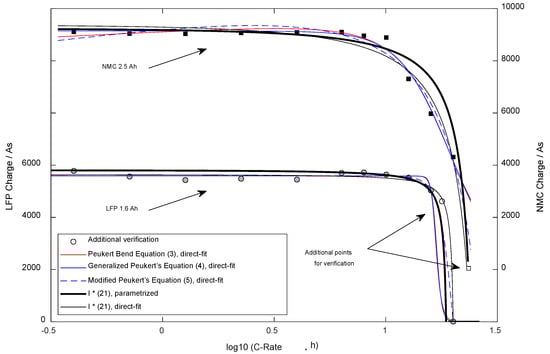
Figure 9.
Available Charge dependent on the discharge current for comparison with equations from literature.
Thirdly, an empirical equation parametrized by fitting without a properly grounded physical model does not allow for extrapolation. As visible in Figure 9, the Peukert Band Equation and the Generalized Peukert’s Equation failed with both cell types, while the fitted Equation (21) and the Modified Peukert’s Equation were able to meet the additional verification point. Additionally, the experimentally parameterized results of (21) perform well when predicting the bends and maximum possible currents for both cell types.
When directly comparing the different equations, the Peukert Bend Equation (DF = 4) and the Generalized Peukert’s Equation (DF = 3) behaved nearly identically. When varying the starting parameters of the fitting processes, it was recognized that the gained shapes were almost identical in most cases. The extra degree of freedom of the Peukert Bend Equation does not lead to any advantage when comparing these two proposals. In contrast to the developed system of equations, both can describe the slightly rising capacity with medium currents in contrast to small currents (temperature effect, the cell is heating up while discharge, internal resistance is reduced and leads to a delayed break-off). Based on the statistics presented in Table 2, these two equations performed best, but practically the usage cannot be recommended due to the unstable behavior and the limited capabilities for extrapolation (for small and high currents).
In contrast, the Modified Peukert’s Equation (DF = 4) also showed good statistics and stability. It seems to allow for inter- and (limited) extrapolation based on the cell types selected for the research. It needs to be mentioned that the fitted parameters and were not employed by the simplex-downhill method (finding the local minimum error) in the published way (refer [18]): For NMC (the current where 50% of the capacity should be available) was fitted to 0.4 A, a value far too small, while was found correctly. For LFP, (the immediate break-off current) was smaller than . Equation (21) does not support the temperature effect and delivers the worse statistics but allows for a stable fitting process and interpolation. For the LFP cell, the parameters were employed by the fitting algorithm in an intended way, while for NMC, for the parameter a negative value was found. Extrapolation should be used carefully when the parameters were gained using direct-fitting, such as with the Modified Peukert’s equation. Usage of (21) with the proposed way of parametrization with independent experiments on the basic parameters does allow for rigid inter- and extrapolation but delivers lower accuracy (Table 2, . The standard error compensated for the degrees of freedom and was nearly identical using both parametrization methods. The graphs and statistics show that the LFP cell type could be described with all tested equations more accurately compared to NMC.
4.3. Peukert Behavior
The presented system implements the main reasons for the decreasing available capacity with growing discharge currents. Generally, the discharge capacity is stable. Thus, the discharge time is inversely proportional to the current. The dominating effect influencing drop conditions with higher discharge currents is the voltage drop on the internal resistance, which rises proportionally to the test current. Thus, the cut-off is triggered at higher SoC than expected. Against that dominating effect, two reasons somewhat delay the cut-off moment for higher currents: First, the open-circuit voltage is higher at higher SoC. Secondly, the internal resistance is reduced.
The research confirms what is already discussed in the literature (e.g., [13]): the classic Peukert exponent is only valid for a limited current range (up to 2–5 Cn). With the presented method, “local” mean Peukert exponents, which are valid for a specific span of discharge currents, can be determined.
The present research demonstrated that this type of equation (comparing the opposite opinion of Tremblay [20]) could indeed describe the Peukert effect well, including the second, stronger decline for very high currents, the so-called Peukert-bend [13]. Furthermore, this bend is just a natural prosecution of the curve (see Figure 4), in which the curvature increases steadily even from small currents (see Figure 5).
In contrast to [13,17,18], the proposed method also describes the main reasons for the bend and allows for the prediction of the bend intensity and bend position for different cell types based on nondestructive measurements in the datasheet range. Instead of enhancing the (empirical) Peukert equation to empirically meet the behavior of lithium-ion batteries at varying currents, usage of (22) is recommended, which forecasts real cell behavior, including the bend at high currents. The presented equations allow for determining the needed parameters for the entire current range without having to repeat several discharge procedures.
Additionally, the proposed system of equations enables the extraction of a current dependent and locally valid “Peukert exponent” by deviating the double logarithmic presentation of (21), presented in (24) and Figure 5. Alternatively, it offers a method to directly determine the Peukert exponent (valid for a specific area of currents) without experimentally performing complete discharge cycles with different currents.
4.4. Outlook
The set of equations also offers the usage for predicting the maximum pulse duration for a given discharge current and SoC. As discrete-time simulations can be omitted, implementation for such purpose on slower µC (as in battery management systems) is recommended.
Additionally, when leaving the direct mathematical method, core equation (13) could function as a base for a further extension with dynamic behavior and for the incorporation of temperature models in discrete-time simulations, as it allows for the calculation of clamp voltage in the future, assuming a constant current for that discrete time.
The results show accurate results based on a single calculation step for a long duration. Thus, using the equations as a base for discrete-time calculations is promising. The authors recommend investigating further the calculation effort for (13) compared to simpler equations, which may need smaller calculation step durations and, thus, higher calculation effort to reach a competitive forecast quality.
5. Conclusions
The shape of an existing Equation (5)—originally intended to describe the OCV—was additionally applied to characterize the internal resistance of lithium-ion cells. Two parameters (, ) describe certain charge positions in the SoC-dependent behavior of the cell types. Therefore, applying these positions/parameters for the OCV and the internal resistance was possible. This step allowed for simplification, which enabled the direct usage of mathematical equations to predict lithium-ion cells’ energy and charge content dependence on the used constant discharge current. Thus, the proposed system avoids the necessity of discrete-time simulations to determine these parameters.
In the present research, the new method (to parametrize the equation delivering the finally needed size by investigating ground laying sizes) was compared with the method of direct fitting. That commonly used way (fitting to samples of the final desired physical dimension) produces, focusing on statistics, more accurate results, but has drawbacks. First, the interpolation results may be lacking depending on the set of experimental results and the employed equation. Thus, automatic cell characterization without manual checks is problematic. Secondly, the extrapolation of fitted equations without a physical basis is not applicable. Third, the experimental series needs a specific density and must cover the full range of currents intended by the creator of the equation to avoid overfitting. This forces safety-critical currents during the parametrization experiments, increasing experimental efforts. Additionally, as currents outside the datasheet range are used, more specimens/channels are necessary to finalize the model.
Using the proposed characterization method and equations, only eight significant and directly physically understandable parameters (, , , , , , plus and ) can be obtained, which characterize the behavior of a specific Li-ion cell type. These parameters allow for simple database storage and comparison, for example, to support automated cell down-selection. Furthermore, the cell characterization can be programmed to run fully automatic on a single specimen and channel (more recommended for redundancy).
Furthermore, in contrast to pure empirical and more or less arbitrary selected equations, the proposed set of equations is based on a battery cell model. Thus, even when the proposed equations were used (different from the new method described in this paper) for direct empirical fitting of the target size (e.g., available capacity), they offer additional advantages over purely empirical equations, such as a stable fit, less necessary experiments, and support for extrapolation.
In conclusion, depending on the researcher’s aims, the new method can provide significant performance, e.g., for fully automatic and fast characterization of a high number of cell types with standard equipment.
Author Contributions
Conceptualization, F.S. and H.-G.S.; methodology, F.S.; software, F.S. and J.K.; validation, H.-G.S., J.K. and L.M.; formal analysis, F.S.; investigation, J.K. and F.S.; resources, H.-G.S.; data curation, F.S. and J.K.; writing—original draft preparation, F.S.; writing—review and editing, L.M., H.-G.S. and J.K.; visualization, F.S.; supervision, L.M. and H.-G.S.; project administration, F.S.; funding acquisition, H.-G.S. All authors have read and agreed to the published version of the manuscript.
Funding
The APC was funded by the Post-Grand-Fund Program of the German Federal Ministry of Education and Research FKZ: 16PGF0163.
Institutional Review Board Statement
Not applicable.
Data Availability Statement
Not applicable.
Acknowledgments
We thank Walter Strasser and Onur Kul for performing the LFP cell measurements and Katja Brade for her helpful suggestions on the manuscript.
Conflicts of Interest
The authors declare no conflict of interest.
References
- Paris Declaration on Electro-Mobility and Climate Change & Call to Action. In Proceedings of the Lima–Paris Action Agenda, UN Climate Change Conference, Paris, France, 29 November 2015; Available online: https://unfccc.int/documents/23227 (accessed on 2 June 2022).
- Cao, D.; Zhang, H.; Du, H. Modeling, Dynamics, and Control of Electrified Vehicles; Woodhead Publishing: Duxford, UK, 2018. [Google Scholar]
- Schuster, S.F.; Brand, M.J.; Berg, P.; Gleissenberger, M.; Jossen, A. Lithium-ion cell-to-cell variation during battery electric vehicle operation. J. Power Sources 2015, 297, 242–251. [Google Scholar] [CrossRef]
- Kulkarni, M.; Vaidya, A.; Karwa, P. I2t derivation for Electrical Safety (EV). IEEE Int. Transp. Electr. Conf. (ITEC) 2015, 133–135. [Google Scholar] [CrossRef]
- Hussein, A.-H.; Batarseh, I. An Overview of Generic Battery Models. In Proceedings of the IEEE PES General Meeting, Detroit, MI, USA, 24 July 2011; pp. 1529–1534. Available online: https://ieeexplore.ieee.org/document/6039674 (accessed on 19 June 2021). [CrossRef]
- Mousavi, S.M.; Nikdel, M. Various battery models for various simulation studies and applications. Ren. Sust. Energy Rev. 2014, 32, 477–485. [Google Scholar] [CrossRef]
- Lu, L.; Han, X.; Li, J.; Hua, J.; Ouyang, M. A review on the key issues for lithium-ion battery in electric vehicles. J. Power Sources 2013, 226, 272–288. [Google Scholar] [CrossRef]
- Liu, K.; Li, K.; Peng, Q.; Zhang, C. A brief review on key technologies in the battery management system of electric vehicles. Front. Mech. Eng. 2019, 14, 47–64. [Google Scholar] [CrossRef]
- González-Longatt, F.M. Circuit-Based Battery Models: A Review; 2 do Congreso Iberoamericano de Estudiantes de Ingeneria Electrica, II Cibelec, 2006. Available online: https://pdfs.semanticscholar.org/5a79/ca86eaea1de96f7c3ea1248ea4b28f55c2f1.pdf (accessed on 19 June 2021).
- Gaizka Saldaña, G.; San Martín, J.I.; Zamora, I.; Asensio, F.J.; Oñederra, O. Analysis of the Current Electric Battery Models for Electric Vehicle Simulation. Energies 2019, 12, 2750. [Google Scholar] [CrossRef]
- Bergveld, H.J.; Kruijt, W.S.; Notten, P.H.L. Battery Management Systems Design by Modelling; Springer: Dordrecht, The Netherlands, 2002. [Google Scholar]
- Peukert, W. Über die Abhängigkeit der Kapazität der Bleiakkumulatoren von der Stromstärke. Elektrotechnische Z. 1897, 20, 287–288. [Google Scholar]
- Nebl, C.; Steger, F.; Schweiger, H.-G. Discharge Capacity of Energy Storages as a Function of the Discharge Current–Expanding Peukert’s equation. Int. J. Electrochem. Sci. 2017, 12, 4940–4957. [Google Scholar] [CrossRef]
- Song, D.; Sun, C.; Wang, Q.; Jang, D.A. Generic Battery Model and its Parameter Identification. Energy Power Eng. 2018, 10, 10–27. [Google Scholar] [CrossRef]
- Yang, A.; Wang, Y.; Yang, F.; Wang, D.; Zi, Y.; Tsui, K.L.; Zhang, B. A comprehensive investigation of lithium-ion battery degradation performance at different discharge rates. J. Power Sources 2019, 443, 227108. [Google Scholar] [CrossRef]
- Omar, N.; Van den Bossche, P.; Coosemans, T.; Van Mierlo, J. Peukert Revisited–Critical Appraisal and Need for Modification for Lithium-Ion Batteries. Energies 2013, 6, 5625–5641. [Google Scholar] [CrossRef]
- Galushkin, N.E.; Yazvinskaya, N.N.; Galushkin, D.N. Analysis of Generalized Peukert’s Equations for Capacity Calculation of Lithium-Ion Cells. J. Electrochem. Soc. 2020, 167, 013535. [Google Scholar] [CrossRef]
- Galushkin, N.E.; Yazvinskaya, N.N.; Galushkin, D.N. A Critical Review of Using the Peukert Equation and its Generalizations for Lithium-Ion Cells. J. Electrochem. Soc. 2020, 167, 120516. [Google Scholar] [CrossRef]
- Yazvinskaya, N.N.; Lipkin, M.S.; Galushkin, N.E.; Galushkin, D.N. Peukert Generalized Equations Applicability with Due Consideration of Internal Resistance of Automotive-Grade Lithium-Ion Batteries for Their Capacity Evaluation. Energies 2022, 15, 2825. [Google Scholar] [CrossRef]
- Tremblay, O.; Dessaint, L.-A.; Dekkiche, A.-I. A Battery Model for the Dynamic Simulation of Hybrid Electric Vehicles. In Proceedings of the IEEE Vehicle Power and Propulsion Conference 2007, Arlington, TX, USA, July 2007; Available online: https://ieeexplore.ieee.org/abstract/document/4544139 (accessed on 15 September 2019).
- Shepherd, C.M. Design of Primary and Secondary Cells: An Equation Describing Battery Discharge. J. Electrochem. Soc. 1965, 112, 657–664. [Google Scholar] [CrossRef]
- Ratnakumar, B.V.; Smart, M.C.; Whitcanack, L.D.; Ewell, R.C. The impedance characteristics of Mars exploration Rover Li-ion batteries. J. Power Sources 2006, 159, 1428–1439. [Google Scholar] [CrossRef]
- Tremblay, O.; Dessaint, L.-A. Experimental Validation of a Battery Dynamic Model for EV Applications. In Proceedings of the EVS24 International Battery, Hybrid and Fuel Cell Electric Vehicle Symposium, Stavanger, Norway, 3 May 2009. [Google Scholar]
- Rodrigues, L.M.; Montez, C.; Moraes, R.; Portugal, P.; Vasques, F. A Temperature-Dependent Battery Model for Wireless Sensor Networks. Sensors 2017, 17, 422. [Google Scholar] [CrossRef] [PubMed]
- Nájera, J.; Moreno-Torres, P.; Lafoz, M.; De Castro, R.M.; Arribas, J.R. Approach to Hybrid Energy Storage Systems Dimensioning for Urban Electric Buses Regarding Efficiency and Battery Aging. Energies 2017, 10, 1708. [Google Scholar] [CrossRef]
- Vötsch Industrietechnik. Vötsch VT4011 Temperature Chamber; Weiss Klimatechnik GmbH: Reiskirchen, Germany, 2015; Available online: http://www.v-it.com/de/home/schunk01.c.59546.de (accessed on 2 May 2020).
- Zahner-Elektrik. ZAHNER PP-Series power potentiostats; Zahner-Elektrik GmbH & Co. KG: Kronach, Germany, 2012. [Google Scholar]
- Array Electronic. Array 372x Series Electronic Load; Array Electronic Co. Ltd.: Nanjing, China, 2018; Available online: http://www.array.sh/yq-3721e.htm (accessed on 2 May 2020).
- Bitrode Corporation. TV/HEV Battery Cell Testing System; Bitrode Corporation: Saint Louis, MO, USA, 2015; Available online: http://www.bitrode.com/model-mcv/ (accessed on 2 May 2020).
- Neware Technology Limited. Cell Battery Tester-18650 CT-4008-5V6A-S1 Battery Testing System User Manual Version 1.0; Neware Technology Limited: Shenzhen, China, 2013. [Google Scholar]
- Samsung SDI. Introduction of INR18650-25R; Samsung SDI Europe GmbH: Ismaning, Germany, 2013. [Google Scholar]
- ENERdan GmbH. HTCFR18650-1600mAh-3.2V Shandong Goldencell Electronics Technology, Product Specifications; ENERdan GmbH: Berlin, Germany, 2021. [Google Scholar]
- De Hoog, J.; Timmermans, J.-M.; Ioan-Stroe, D.; Swierczynski, M.; Jaguemont, J.; Goutam, S.; Omar, N.; Van Mierlo, J.; Van Den Bossche, P. Combined cycling and calendar capacity fade modeling of a Nickel-Manganese-Cobalt Oxide Cell with real-life profile validation. Appl. Energy 2017, 200, 47–61. [Google Scholar] [CrossRef]
- Keil, P.; Jossen, A. Aufbau und Parametrierung von Batteriemodellen. September 2018. Available online: https://mediatum.ub.tum.de/doc/1162416/1162416.pdf (accessed on 2 August 2020).
- PHP: Hypertext Preprocessor. Available online: http://php.net (accessed on 2 June 2020).
- ISO 12405-1; 7.3 Power and Internal Resistance. International Organization for Standardization: Geneva, Switzerland, 2011.


Publisher’s Note: MDPI stays neutral with regard to jurisdictional claims in published maps and institutional affiliations. |
© 2022 by the authors. Licensee MDPI, Basel, Switzerland. This article is an open access article distributed under the terms and conditions of the Creative Commons Attribution (CC BY) license (https://creativecommons.org/licenses/by/4.0/).