Forecasting Day-Ahead Carbon Price by Modelling Its Determinants Using the PCA-Based Approach

Abstract

Accurate price forecasts on the EU ETS market are of interest to many production and investment entities. This paper describes the day-ahead carbon price prediction based on a wide range of fuel and energy indicators traded on the Intercontinental Exchange market. The indicators are analyzed in seven groups for individual products (power, natural gas, coal, crude, heating oil, unleaded gasoline, gasoil). In the proposed approach, by combining the Principal Component Analysis (PCA) method and various methods of supervised machine learning, the possibilities of prediction in the period of rapid price increases are shown. The PCA method made it possible to reduce the number of variables from 37 to 4, which were inputs for predictive models. In the paper, these models are compared: regression trees, ensembles of regression trees, Gaussian Process Regression (GPR) models, Support Vector Machines (SVM) models and Neural Network Regression (NNR) models. The research showed that the Gaussian Process Regression model turned out to be the most advantageous and its price prediction can be considered very accurate.

1. Introduction

The possibility of predicting European Union Allowance (EUA) price level is extremely important, especially from the viewpoint of companies whose production process is inherently related to carbon dioxide (CO₂) emissions. As part of the European Union Emission Trading System (EU ETS), these entities are tasked with reducing their CO₂ emissions, but in the case of no action being taken against CO₂ emitting, they must settle this with purchased or assigned EUA units. This applies to both the energy sector using non-renewable fuels and companies from cement, refinery, coke sectors and many other industry sectors in which emissions occur in the production process. Moreover, this market has become attractive in terms of investment, which has resulted in the accession of many financial entities such as banks and investment funds. This increased the number of participants in the system, which resulted in a greater trading volume and the unpredictability of prices. In recent months, EUA prices have reached over EUR 90 per ton and are already over 150% more expensive than at the beginning of 2021. This has made the CO₂ emissions trading system a costly burden, especially for industry and energy which depend on coal. For this reason, the knowledge of the problem of price volatility of CO₂ emissions and the possibility of its prediction has become necessary to make profitable decisions by entrepreneurs and, therefore, it is a complex issue that requires a scientific approach.

According to [1] prediction models for carbon price developed so far are divided into these types:

-

prediction model using the econometric method;

-

prediction model based on artificial intelligence algorithms;

-

combined prediction model.

The traditional statistical and econometric models are widely used for carbon price forecasting. The first group includes IA models for price volatility expanding the scope from models of type Generalized Autoregressive Conditional Heteroskedasticity (GARCH) to models with long-term dependence and regime switches including the class of so-called multifractal models. Ref. [2] used a non-parametric method to estimate carbon prices and found that the method could reduce the prediction error by almost 15% compared with linear autoregression models. Ref. [3] applied multivariate GARCH models to estimate the volatility spillover effects amongst the spot and futures allowance markets during the Phase II period. Different GARCH-type models to predict the volatility of carbon futures were explored by [4]. The conditional variance of carbon emissions prices using various GARCH models was examined by [5]. Ref. [6] point out the suitability of applying asymmetric GARCH models for modelling the volatility of carbon allowance prices. Ref. [7] applied these models to carbon dioxide emission allowance prices from the European Union Emission Trading Scheme and evaluated their performance with up-to-date model comparison tests based on out-of-sample forecasts of future volatility and value at risk. Ref. [8] developed a combination-MIDAS regression model to perform real-time forecasts for the weekly carbon price, using the latest revealed high-frequency economic and energy data. The authors analyze the forecasting interactions among carbon price, economic and energy variables at the mixed frequencies, and assess the nowcasting performances of the combination-MIDAS regression models by comparing the root mean squared errors (RMSE). Ref. [9] used asymmetric GARCH processes (EGARCH and GJR-GARCH) to model the asymmetric volatility in emission prices and analyzed how good and bad news impact the EUA market volatility under structural breaks.

The second group of models includes IA a short-term prediction model based on Neural Networks for forecasting carbon prices of the European Union Emissions Trading Scheme in phase III. Ref. [10] have proposed a Multi-Layer Perceptron (MLP) network model, based on the reconstruction technique of phase space. Ref. [11] proposed the following computational intelligence techniques: a novel hybrid neuro-fuzzy controller with a closed-loop feedback mechanism (PATSOS); a neural network-based system; and an adaptive neuro-fuzzy inference system (ANFIS). This is the first approach to putting a hybrid neuro-fuzzy controller into forecasting carbon prices. Whereas [12] proposed, for carbon price forecasting, a novel multiscale nonlinear ensemble leaning paradigm incorporating Empirical Mode Decomposition (EMD) and Least Square Support Vector Machine (LSSVM) with a kernel function prototype. Ref. [1] developed presented a new carbon price prediction model applied by using a time series complex network analysis technology and an extreme learning machine algorithm (ELM). In that model, the authors’ first stage map of the carbon price data was mapped into a carbon price network (CPN). In the second stage, the effective information of carbon price fluctuations by net-work topology is extracted and the extracted effective information is applied to reconstruct the carbon price sample data.

Ref. [13] proposed several novel hybrid methodologies that exploit the unique strength of the traditional Autoregressive Integrated Moving Average (ARIMA) and the least squares support vector machine (LSSVM) models in forecasting carbon prices. Additionally, Particle Swarm Optimization (PSO) is used to find the optimal parameters of LSSVM to improve the prediction accuracy. An empirical mode decomposition-based evolutionary least squares support vector regression multiscale ensemble forecasting model for carbon price forecasting was proposed in the study of [14]. To obtain better estimation results, a hybrid model conjunctive Complete Ensemble Empirical Mode Decomposition (CEEMD), Co-Integration Model (CIM), GARCH and Grey Neural Network (GNN) with Ant Colony Algorithm (ACA) was presented by [15]. Ref. [16] developed a hybrid decomposition and integration prediction model using the Hodrick–Prescott filter, an improved grey model and an extreme learning machine.

The EMD–GARCH model that combined integrated empirical mode decomposition (EMD) with generalized autoregressive conditionally heteroskedastic (GARCH) was presented by [17] to forecast the carbon price of the five pilots (Shenzhen, Shanghai, Beijing, Guangdong and Tianjin) in 2016. The mode decomposition and GARCH model integrated with a Long Short-Term Memory (LSTM) network for carbon price forecasting was proposed in a more recent publication [18].

Two main trends can be distinguished from the approaches mentioned above: methods in which EUA price prediction is based on time-series data using price-only forecasting (for example [2,3,18]) and methods that use factors influencing the EUA price prediction (for example [8,19]).

Ref. [7] have focused their studies on the significance of energy prices (oil, gas, coal and electricity) and weather (temperatures and radical weather phenomenon) in the influence of carbon prices. Ref. [20] explored vital factors with an impact on the price of emission allowances in the EU trading system in the years 2005–2007. They analyzed the policy, regulations and market factors: weather and production levels with technical indicators.

Ref. [19] developed a model to predict daily carbon emissions price changes by taking the analysis rationality of pricing behavior based on weather and non-weather variables. Ref. [21] proved that energy prices and EUA prices can affect each other. Ref. [22] identified several macroeconomic drivers of EUA prices and examined the correlation between the return on carbon futures and changes in macroeconomic conditions. Ref. [23] described a significant correlation between carbon prices and stock prices and the index of industrial production. Ref. [24] indicated that a shock in the EUR/USD exchange rate has an influence on the carbon credit market. Ref. [25] applied to the carbon price forecast an artificial neural network (ANN) algorithm based on coal, the S&P clean energy index, the DAX index and other variables. Ref. [26] applied a semiparametric quantile regression model to explore the effects of energy prices (coal, oil and natural gas prices) and macroeconomic drivers on carbon prices at different quantiles.

Thus, according to the literature, there are many non-weather factors that affect the formation of EUA prices. Most analyses, however, are concerned with select indicators and individual stock exchange contracts representing selected products. The aim of the study is to jointly analyze a wide range of fuel and energy indicators, which are contracts determining EUA price trends, and to find an EUA price prediction methodology that will be best to forecast their daily course based on the analyzed set of factors. To address multiple gaps, the contribution of our paper is:

a. Thanks to a careful analysis of 2021,the first year from 4th EU ETS period, which characterized by very high volatility, the work indicates directions of correlation between EUA prices and the prices of other contracts on the fuel and energy market, what can be used to make additional research studies by researchers or could be directly used by industrial plants involved in emissions trading. This is the latest scope of analyzes concerning the EU ETS system changed after period III, which has not been the subject of research by other scientists so far.

b. Another novelty is the wide input data set for the analysis of the EUA price determinants. The applied mathematical models, thanks to which hundreds of data were analyzed, allowed for a significant narrowing of the set as an input data to prediction models. It was considered in this study, as the most important from the point of view of forecast models’ complexity.

c. Non-price factors, such as the impact of decisions shaping the rules of the EU ETS market, for which we proved that had only a limited, short-term impact on EUA prices, were not investigated in similar research.

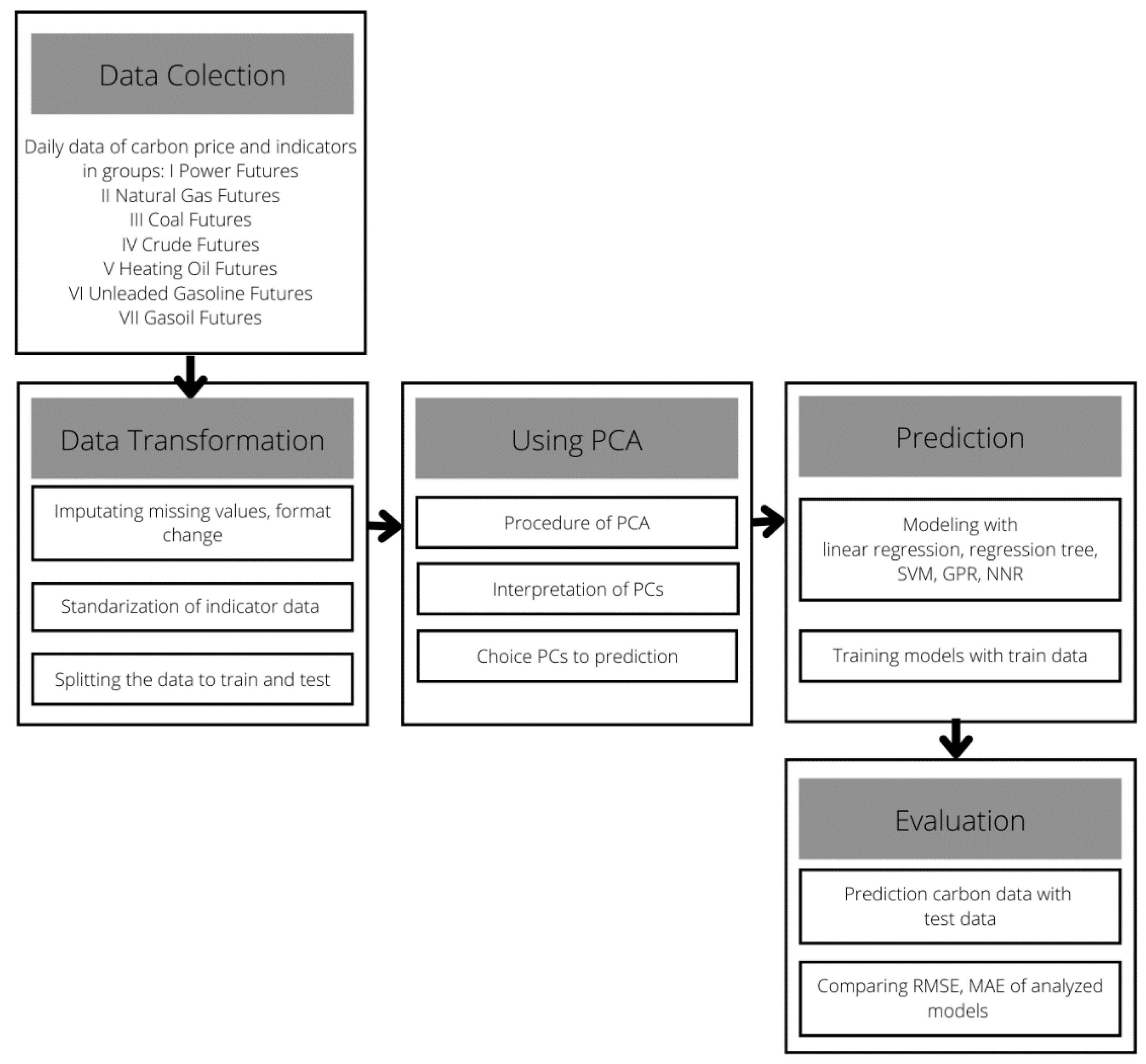
In the proposed approach, by combining the Principal Component Analysis (PCA) method and selected methods of supervised machine learning, the possibilities of predicting the numerical value of the emission price in the period of its rapid growth are explored. The PCA method allows the reduction of the number of variables to the ones used as inputs for predictive models. It also allows this study to list the factors with the decisive value of the variance of the analyzed data space. Among the supervised machine learning methods, these models are compared: regression trees, ensembles of regression trees, Gaussian Process Regression (GPR) models, Support Vector Machines (SVM) models and Neural Network Regression (NNR) models.

There are also studies that use forecasting models in other fields to show the interdisciplinary use of forecasting methods. Ref. [27] described a functional forecasting method. In particular, a functional autoregressive model of order P is used to a short-term energy price prediction. The authors propose using a functional final prediction error as a way to selection of the model dimensionality and lag structure. Energy price forecasting is also described in the work of [28], which proposes a forecasting framework based on big data processing, which selects a small quantity of data to achieve accurate forecasting while reducing the time cost. Price forecasting is difficult due to the specific features of the electricity price series, Ref. [29] examined the performance of an ensemble-based technique for forecasting short-term electricity spot prices in the Italian electricity market (IPEX). On the other hand, Ref. [30] proposed a novel interpretable wind speed prediction methodology named VMD-ADE-TFT, which was used to improve the accuracy of forecasts. Ref. [31], in a further study, described forecasting the U.S oil markets based on social media information during the COVID-19 pandemic. In the studies cited above, it was shown that deep learning can extract textual features from online news automatically. Ref. [32] performed a comparative analysis for daily peak load forecasting models. They compared the performance of time series, machine learning and hybrid models. The authors proved that hybrid models show significant improvements over the traditional time series model, and single and hybrid LSTM models show no significant performance differences.

The paper is organized as follows: Section 2 presents works related to the theory of the PCA method. The overall framework of the methodology of the study is demonstrated in Section 3. Section 4 analyzes the data used. The experimental results of the proposed approach and discussion about it are presented in Section 5. The conclusions are reported in the last section.

2. Related Work

2.1. PCA Method

Principal Component Analysis (PCA) is one of the factor analysis methods proposed by [33], which is used for dimensionality reduction and feature extraction. In the method, a set of data as a cloud of N points in a K-dimensional space (N observations for K indicators for EUA price) is analyzed by rotating the coordinate system to maximize the variance, starting with the first coordinate, then the second, and so on. This way, the set of principal components (PCs) is generated equal to the number of the analyzed indicators. However, the variance of the parameters is different, and most often, the first few PCs describe over 99% of the variance. Thus, the number of variables can be reduced without losing too much information [34]. According to [35], the PCA is one of the most-cited data-based multivariate statistical methods in the literature.

The steps of the PCA method are:

Step. 1. Standardization

Standardization is a critical step of the analysis because a different range of data for different indicators means that the variance of these variables is not comparable. Standardization is carried out as follows:

$$r_{kn}=\frac{x_{kn}-m\left(x_k\right)}{dev\left(x_k\right)}$$

(1)

where $x_{kn}$ is a value of nth observation for kth indicator, $m\left(x_k\right)$ is an arithmetic mean of kth indicator values and $dev\left(x_k\right)$ is a standard deviation of values for kth indicator. Thus, matrix $R=\left\{r_{kn}:k=1,\dots K,n=1,\dots ,N\right\}$ is the matrix of standardized values of nth observation for kth indicators.

Step. 2. Covariance matrix computation

To identify correlations between indicators, a covariance matrix S of the size KxK: is calculated:

$$S=\left[\begin{array}{c}\begin{array}{ccc}Cov\left(r_1, r_1\right)& \begin{array}{cc}Cov\left(r_1, r_2\right)& \dots \end{array}& Cov\left(r_1, r_K\right)\\ Cov\left(r_2, r_1\right)& \begin{array}{cc}Cov\left(r_2, r_2\right)& \dots \end{array}& Cov\left(r_2, r_K\right)\\ \cdots & \cdots & \cdots \end{array}\\ \begin{array}{cc}\begin{array}{cc}Cov\left(r_K, r_1\right)& Cov\left(r_K, r_2\right)\end{array}& \begin{array}{cc}\dots & Cov\left(r_K, r_K\right)\end{array}\end{array}\end{array}\right]$$

(2)

where $Cov\left(r_i, r_j\right)$ is the coefficient of covariance for the pair (ith and jth standardized indicators).

Step. 3. Calculation of eigenvectors and eigenvalues

Let v be a vector and λ a scalar that satisfies $S\mathsf{\nu } = \mathsf{\lambda }\mathsf{\nu }$, then λ is an eigenvalue associated with eigenvector ν of S. After adaptation of the equation, we obtain:

(S − λI)ν = 0

(3)

where I is the (KxK) identity matrix. By solving Equation (3) for different values of λ eigenvalue, we obtain the matrix of eigenvectors. To decide which eigenvector is maximizing the v value, the λ value must be as large as possible [36]. Hence $\mathrm{var}\left(v\prime \mathrm{R}\right)=v\prime \mathrm{S}v=\mathsf{\lambda }$ (the largest eigenvalue).

There are several algorithms used for calculations in the PCA method. These are IA SVD (Singular Value Decomposition), EIG (EIGenvalue decomposition), ALS (Alternating Least Squares) and NIP ALS (NonIterative Partial Least Squares). One of the most commonly used is the SVD algorithm [37,38].

Step. 4. Determine PCs

The kth principal component $P{C}_k$ of matrix R constitutes $v{\prime }_{k}R$ where var($v{\prime }_{k}R)={\mathsf{\lambda }}_k$, the kth largest eigenvalue of S and $v_k$ is a corresponding eigenvector ($k=1,\dots ,K$) [36]. In the assumption of the method, all PC vectors are uncorrelated with one another. Ultimately:

$$P{C}_k=v{\prime }_{k}R = v_{k1}{r}_{k1}+v_{k2}{r}_{k2}+\dots +v_{kK}{r}_{kK}$$

(4)

where $v_{kK}$is a coefficient (constant) and $r_{kK}$ is an element of matrix R ($k=1,\dots ,K$).

We sort the eigenvectors according to the descending order of their eigenvalues, then we sort the principal components in descending order by their variance (transferred information). To identify the input variables $z_p$, those PCs are selected for which the considered cumulative variance is greater than the assumed value of 95–99%. Thus, $z_p=P{C}_p$ where $p=1,\dots ,P$ and $P\ll K$.

Thus, the method allows to avoid serious collinearity of many variables while minimizing information loss, but also to reduce the complexity of the model and improve the efficiency of the prediction model [37]. After using the PCA method, we obtain a new set of variables that potentially affect the EUA prediction. However, they are other variables often not directly interpretable. To look for a substantive interpretation of the impact of selected indicators on the EUA, it is proposed to use the analysis of association rules as ordered fuzzy numbers. Such an interpretation will facilitate the analysis of data and increase the quality of the decision-making process.

2.2. Selected Supervised Machine Learning Method

Due to the transparency and extensive scope of the paper subject, the methods used are described only briefly, without considering the detailed methodology of calculations. Additionally, since these methods are widely used, we refer to the source literature for these approaches.

2.2.1. Regression Trees

The regression trees, first introduced by [39], are an inverted tree structure that helps predict responses to given inputs. The tree structure is learned based on the training data, considering the assumed conditions, i.e., the minimal number of leafs, and, in our paper, the mean squared error as the splitting criterion. Target regression trees can be truncated to optimize its size and fit the data. To predict the response, we should follow the tree structure from the root node (beginning node) to the last down leaf. In the paper, we consider binary trees. This means that each step in a prediction at each node involves checking the value of one predictor variable (indicator) and deciding what branch to follow down. The last leaf node determines the predicted response.

To improve the predictability and performance of the model, a regression tree ensemble can be used. It is a model, which comprises a weighted combination of multiple regression trees. A boosted regression tree is generated by using the Least-Squares Boosting algorithm (LSBoost) [40]. A bootstrap aggregation (bagging) allows you to generate some bagged regression trees [41]. A random forest technique improves the accuracy of bagged trees [42]. The result of using the optimization with above mentioned algorithms is the ensemble regression with the minimum estimated cross-validation loss [43].

2.2.2. Gaussian Process Regression Model

The Gaussian process regression (GPR) model is a nonparametric kernel-based probabilistic model. It is widely used in applications, especially in non-linear processes, because of their flexibility in the representation form, the possibility of incorporating prior knowledge (kernels) and recognizing the uncertainty over predictions [44] (; [45] and computational simplicity [46]. For this purpose, latent variables, $f(x_i)$, $i=1,2,\dots ,n$, from a Gaussian process and explicit basis functions h are introduced in the probabilistic model:

$$P(y|f,X)~N(y|H\beta +f,{\sigma }^{2}I)$$

(5)

where $y$, $f,$ $X,$ $H$, $\beta$ are vectors of response variables, random latent variables, vectors of input observations, basis functions and coefficients estimated for linear regression model, respectively. In the model, the joint distribution of the latent variables in vector $f$ is close to linear regression model:

$$P(f|X)~N(f|0,K\left(X,X\right))$$

(6)

with n-dimensional matrix of covariance function $K\left(X,X\right)$.

2.2.3. Support Vector Machine Model

The Support Vector Machine (SVM) algorithm is a supervised, non-parametric machine learning algorithm. SVM classifies data by finding the best hyperplane that separates data points of other classes. It is perhaps the most popular and the most widely investigated because it is efficient, insensitive to overtraining, its complexity is not dependent on dimensions and choosing the right kernel function is highly effective in practice [43].

Let consider the following linear function:

$$f\left(x\right)=x_n^T\beta +b.$$

(7)

The SVM model, as a linear ε -insensitive SVM regression, can be described as constrained optimization problem with training input-output data and the following primal formula:

$$J\left(\beta \right)=C{{\displaystyle \sum }}_{n=1}^N\left({\xi }_n+{\xi }_n^{*}\right)+({\beta }^T\beta )/2$$

(8)

where $C$ is a box constraint, ${\xi }_n\ge 0, {\xi }_n^{*}\ge 0$ are slack variables and for each n: $y_n-\left(x_n^T\beta +b\right)\le \mathsf{\epsilon }+{\xi }_n$, $(x_n^T\beta +b)-y_n\le \mathsf{\epsilon }+{\xi }_n^{*}$.

In our research, we use also nonlinear SVM regression model, which replaces the dot product $(x^{T}x$) with non-linear kernel function $K(x^{T}x$) such as Gaussian function $K(x^{T}x)=\exp \left(-\parallel x_j-x_k{\parallel }^2\right)$ and polynomial function $K(x^{T}x)={\left(1+x_j^{\prime }{x}_k^{}\right)}^q$ with $q\in \left\{2,3\right\}$.

2.2.4. Neural Network Regression Method

In this paper, we employed the feedforward neural network as a regression method. It is the most basic neural network [47], which is included to supervised machine learning methods. The neural network consists of an input layer, at last one hidden layer and output layer. In each layer there are neurons interconnected to other neurons of different layers. Each neuron has its own activation function and weight, whose value is selected on a learning process basic by optimizing weights to minimize prediction error (in our research, root mean squared error). Neural networks are an easy-to-use, widely applicated (also in energy problem e.g., [28] modeling technique with a very good ability to map complex functions, especially non-linear ones.

3. Methodology

3.1. Overall Framework

The flow chart of the carbon prices forecasting methodology proposed in this paper is shown in Figure 1. The steps are explained as follows.

3.2. Collection and Transformation of the Data

The data set includes the carbon futures of the EU ETS with fuel and energy indicators from liquid European markets as traded on the ICE (Intercontinental Exchange), which are collected from the www.theice.com website (accessed on 8 August 2022). Among the available markets, it has the greatest liquidity under the EU ETS. The data, as a csv file, has been processed using original procedures written in Visual Basic for Application. Due to the of using the procedures, matrices with data for the analyzed indicators and EUA prices have been obtained. Subsequently, duplicate indicators and data that do not meet the condition of minimal data variability (<10%) have been rejected. A set of 37 indicators with row daily data is used in the appropriate research. The data is divided into seven groups of fuel and energy contracts were selected (

Table 1. List of indicators in product groups.

I Power Futures	II Natural Gas Futures	III Coal Futures	IV Crude Futures
‘UBLUKPowerBaseloadFutureGregorian’ ‘UPLUKPowerPeakloadFutureGregorian’ ‘AOTAustrianPowerFinancialBaseFuture’ ‘AOUAustrianPowerFinancialPeakFuture’ ‘BEBBelgianPowerFinancialBaseFuture’ ‘BEPBelgianPowerFinancialPeakFuture’ ‘DPADutchPowerPeakLoad820Futures’ ‘DPBDutchPowerBaseLoadFutures’ ‘FNAFrenchPowerFinancialPeakFuture’ ‘FNBFrenchPowerFinancialBaseFuture’ ‘GABGermanPowerFinancialBaseFuture’ ‘GAPGermanPowerFinancialPeakFuture’ ‘IPBICEEndexItalianPowerBaseloadFuture’ ‘IPPICEEndexItalianPowerPeakloadFuture’ ‘NLBDutchPowerFinancialBaseFuture’ ‘NLPDutchPowerFinancialPeakFuture’ ‘NRBNordicPowerFinancialBaseFuture’ ‘SPBSpanishPowerFinancialBaseFuture’ ‘SWBSwissPowerFinancialBaseFuture’	‘MUKNaturalGasNBPFuture’ ‘TFUDutchTTFGas1stLineFinancialFuturesUSDMMBtu’ ‘UKDUKNBPGas1stLineFinancialFuturesUSDMMBtu’ ‘AVMAustrianCEGHVTPGasFutures’ ‘IGAICEEndexItalianPSVNaturalGasFuture’ ‘TFMDutchTTFNaturalGasBaseLoadFutures’	‘AFRRichardsBayCoalFuture’ ‘ATWRotterdamCoalFuture’ ‘GCFglobalCOALRBCoalFuture’ ‘M42M42IHSMcCloskeyCoalFutures’ ‘NCFgcNewcastleCoalFuture’	‘DBIDubai1stLineFuture’ ‘HOUPermianWestTexasIntermediateWTICrudeOilFuture’ ‘TWestTexasIntermediateLightSweetCrudeFuture’
V Heating Oil Futures	VI Unleaded Gasoline Futures	VII Gasoil Futures
‘ONewYorkHarborHeatingOilFuture’‘O67HeatingOilOutrightNYHULSHOFuture’	‘NNewYorkHarborUnleadedGasolineFuture’	‘GGasoilFutureLowSulphurGasoilFuturesFromFebruary2015ContractMon’

), which are closely related to the CO₂ emissions market. Primary trade of commodities is carried out by the same group of recipients who, based on legal regulations, have been obligatorily included in the EU ETS. Due to the need to hedge their market positions for the purchased commodities, entities will conclude contracts for the purchase of EUAs in the amount depending on the level of production carried out with a specific type of fuel. The price on the fuel market may cause producers to switch from one type of fuel to another. The procedure of fuel-switching to use a cheaper one, regardless of emissions, will cause additional demand for EUAs. Another market dependence concerns electricity prices, which are indirectly related to the EUA prices. Electricity producers using non-renewable fuels for generation includes the purchase cost of EUAs in the selling price of electricity. These producers are a group of emitters who do not receive (like some industrial plants) free allowances for CO₂ emissions and must cover each tonne of CO₂ produced by purchasing EUAs. Therefore, they constitute a significant part of primary EUAs buyers. Another important group of EUAs traders are investors who exchange EUAs only for profit and their market behavior is driven by the general condition on the EU ETS and related markets. These mentioned factors were the basis for selecting a group of contracts, which correlation was then verified by mathematical methods. There are several contracts on the ICE exchange, which constituted a set of input data for the analyses performed. All selected contracts belonging to the groups mentioned in Table 1, due to the market structure, might depend on each other.

The validity of the models proposed is tested by the real carbon market data. We use the daily European Union Allowance futures prices from the last year (2021). Data is standardized in terms of the format, especially the date format, and checked for deficiencies. Missing data is replaced with the average prices for the last three days. The data set is divided into two subsets: a training set and a testing set. The training set is used to estimate the prediction models parameters. The testing set is used to evaluate the established models. The details and descriptive analysis of the dataset are described in Section 4.

3.3. The Use of PCA Method

The Principal Component Analysis described in Section 2 is used to compress data sets of carbon price indicators into lower dimensionality, so the prediction models used are simpler, more efficient and take less time to learn and draw conclusions. The replacement variables created will be used as inputs for the analyzed predictive models. In addition, the PCA method can analyze the importance of indicators from the perspective of the possibility of carrying as much information as possible (maximizing data variance).

3.4. Carbon Prediction

In this paper, we used the most popular supervised machine learning to explore the possibilities of short-term carbon price prediction using a wide set of factors traded on the Intercontinental Exchange market. The tested models include regression trees, ensembles of regression trees, Gaussian Process Regression (GPR) models, Support Vector Machines (SVM) models and Neural Network Regression (NNR) models, which are widely used in forecasting [34]. The structures and their parameters are chosen arbitrarily and optimized according to hyperparameters with a proper loss function.

3.5. Evaluation

To test the effect of prediction models as loss functions, we used mean square error (MSE) during the optimization of models. We also used root mean square error RMSE:

$$MSE=\frac{{{\displaystyle \sum }}_{t=1}^N{\left(z_t-\widehat{z_t}\right)}^2}{N}, \mathrm{RMSE}=\sqrt{MSE}$$

(9)

where $z_t$ is a real value of variable in time t, $\widehat{z_t}$ is a predicted value of variable in time t, N–is the number of observations.

Due to RMSE inflating errors for data with large outliers [48], we also provide errors in the form of mean of the absolute values of the residuals (MAE):

$$MAE=\frac{{{\displaystyle \sum }}_{t=1}^N\left|z_t-\widehat{z_t}\right|}{N}$$

(10)

4. Data Description

As mentioned above, the data set includes the carbon futures of the EU ETS with fuel and energy indicators from the ICE market. We use daily data from 4 January 2021 through 22 November 2021. This yields a total sample of 8740 observations for all indicators. The daily time series of EUA futures prices are obtained by rolling over future contracts for the delivery date. The delivery date is December of 2021 (DEC21). The details of carbon price data set are presented in Figure 2. The probability density function for the extreme value distribution with location parameter µ = 50.3917 and scale parameter σ = 107.89 is presented in Figure 2a and the description analysis of this dataset is presented in Figure 2b. A daily observation of carbon price in the analyzed time of 2021 is depicted in Figure 3.

The reference year 2021 was in an upward trend for EUA prices (Figure 3). This was affected by the analyzed determinants from the fuel and energy markets and several additional macroeconomic factors, such as political decisions related to the tightening of CO₂ emissions limits for the subsequent years of the system’s operation, market sentiment prevailing among traders and high in relation to the remaining years of the EU ETS operation–inflow of new financial investors who secured their positions by purchasing long-term EUA contracts. This was also the year that manufacturing companies reopened after the downturn caused by the COVID-19 pandemic. This entailed an increase in production, which translated into an increased demand for EUA from industrial producers and the energy sector. Rising gas prices made its use as fuel unprofitable and some plants switched to cheaper coal, emitting more CO₂, which was another factor increasing the entrepreneurs’ demand for EUAs for compliance purposes.

In this paper, we also consider 37 indicators that may affect the carbon price. The indicators are analyzed in groups for individual products (Table 1). Figure 4 shows descriptive statistics charts for the analyzed indicators. Figure 5 presents a matrix of correlation coefficients. The correlation among all indicators and EUA is higher than 0.7. A higher correlation (>0.9) can be seen between the indicators in the same product group. A high correlation is also observed between the prices of power and natural gas and the prices of crude, heating oil, unleaded gasoline and gasoil. The exception is the correlation between the x17 contract (‘NRBNordicPowerFinancialBaseFuture’) and other prices of power and natural gas. From the group of contracts for the supply of electricity, this contract shows the lowest convergence. This is because producers from Nordic countries are not as dependent on fossil fuels as elsewhere in Europe. Electricity in the Nordic region is generated largely from renewable resources (mainly hydro and wind power).

5. Experimental Results and Discussion

5.1. Principal Component Analysis

For indicators from Table 1, the PCA method was applied. The variance of data was explained by a relatively small number of PCs (four), which resulted in the selection of four components that should affect the EUA price in 2021. The method reduced the number of input variables for some predictive model to about 10%. The first PC explains over 93% of variance and four first PCs explain together 99.6% of variance (Figure 6). Figure 6 presents the results of the PCA method. The details in the table show how much the 15 principal components describe the overall variance of the indicators.

Figure 7 graphically presents the coefficients (contents) v in formula (4). In the interpretation of the results obtained by use of the PCA, the meaning of each primary indicators in a PC can be determined. The higher the modulus value of an element in the eigenvector, the more important this variable for a PC is.

In PC1, all the coefficients of indicators are positive and not very differentiated; thus, all parameters are positively correlated with the main component that most describes the total variance of the analyzed data. However, these indicators can be identified as having the greatest impact on over 93% of the total variance for the model. These are x1–x16 x18–x25, thus, the products of groups I and II (I Power Futures and II Natural gas Futures).

However, the PC2 with a positive correlation is mainly affected by the variables from the last four groups: IV Crude Futures, V Heating Oil Futures, VI Unleaded Gasoline Futures and VII Gasoil Futures. For the other two groups of indicators, the coefficients are much lower and negative.

The component PC3 mainly represents indicators from the III Coal Futures group and the x17 “NRBNordicPowerFinancialBaseFuture” contract, the values of the remaining indicators negatively affect this input variable, with the largest negative ratio being x9 “FNAFrenchPowerFinancialPeakFuture”.

The indicator “NRBNordicPowerFinancialBaseFuture” is the main factor affecting the value of the fourth surrogate variable (PC4) in prediction models.

To examine which indicators have the greatest impact on the described information, we used the weighted sum of the coefficients for PC1-PC4 modules, where the weights are the percentages of variance described by individual PCs. The results obtained are presented in Figure 8. The values are very close to each other. The analysis shows that the lowest impact on the described information is due to these indicators: x17 “NRBNordicPowerFinancialBaseFuture”, x26 “AFRRichardsBayCoalFuture”, x28 “GCFglobalCOALRBCoalFuture” and x29 “M42M42IHSMcCloskeyCoalFutures”, hence mainly the indicators from the group III “Coal Futures”.

5.2. Forecasting Day-Ahead Carbon Price by Use of PCA-Based Approach with Supervised Machine Learning

This section presents the use of various predictive data mining methods to explore the possibility of day-ahead predictions of EUA prices based on fuel and energy factors and comparison of methods in this application. The surrogate variables created in the PCA method $z_p$ ($p=1,\dots ,4)$constitute inputs for selected prediction methods. The following supervised machine learning techniques are used: regression trees, ensembles of regression trees, Gaussian Process Regression (GPR) models, Support Vector Machines (SVM) models and Neural Network Regression (NNR) models.

To identify the models, daily datasets for carbon price and standardized datasets of 37 indicators (in day-ahead) were randomized into training data and testing data (in 80%/20% ratio). A set of 184 total observations of training data and 46 observations of testing data were obtained. The models were trained using cross-validation with five folds. The cross-validation methodology provides a good estimate of the accuracy of the model prediction after learning with the training dataset. The method uses all data but creates repeated matches. Hence, it is suitable for smaller datasets, like our case. However, multiple matches cause the errors for the training data to be higher than for the model trained once on one dataset, but the predicted accuracy of the model for the testing data is higher because overtraining is avoided. The calculations were made in Matlab and Statistics and Machine Learning Toolbox.

Table 2. Prediction errors with decision trees and ensemble trees.

Model Type		Validation Results				Test Results
		RMSE (Validation)	R-Squared (Validation)	MSE (Validation)	MAE (Validation)	RMSE (Test)	R-Squared (Test)	MSE (Test)	MAE (Test)
Decision Tree	Medium Tree (leaf size: 12)–optimizable model	1.9865	0.96	3.9461	1.4795	2.2604	0.94	5.1092	1.7735
	Simple Tree (leaf size: 5)	2.1766	0.95	4.7376	1.5339	1.9614	0.95	3.8471	1.557
	Medium Tree (leaf size: 13)	2.0003	0.96	4.0012	1.5277	2.2242	0.94	4.9469	1.7721
	Coarse Tree (leaf size: 37)	3.4097	0.87	11.626	2.6714	3.9808	0.81	15.847	3.3221
Ensemble Tree	Boosted Trees (leaf size: 9)	2.7128	0.92	7.3592	2.2736	2.9867	0.89	8.9207	2.4125
	Bagged Trees (leaf size: 9)	1.9771	0.96	3.909	1.5253	2.1909	0.94	4.8002	1.7552
	Ensemble Tree (Bag, leaf size: 3) optimizable model	1.6553	0.97	2.7402	1.2679	1.7114	0.97	2.9288	1.34

presents the results of carbon price predictions with decision tree methods. A decision tree is a hierarchical model composed of decision rules that recursively split independent variables into homogeneous zones [49]. The literature presents many decision tree applications in real classification and prediction problems. It is a method that requires little memory and training time. The method is also easy to interpret, but due to the large granularity of the output information, it often has a low accuracy of prediction. Table 2 presents the prediction results for selected simple, medium and complex size decision tree structures and the model fitted with Bayesian optimization to minimize the MSE error function (9). Here, simpler models work better, but their prediction accuracy is not the greatest. Using functional forms of ensemble models such as boosted trees and bagged trees helped slightly. The boosted tree is a model which creates an ensemble of medium decision trees using the LSBoost algorithm. The bagged tree is a bootstrap-aggregated ensemble of complex decision trees [50]. Among the models, the bagged decision tree has the highest accuracy rate (RMSE 1.6553 for training data and RMSE = 1.7114 for testing data). This model has been adjusted with Bayesian optimization in terms of minimizing the RMSE error by Bag and LSBoost algorithms and these conditions: number of learners: 10–501, learning rate: 0.001–2, minimum leaf size: 1–93 and number of predictors to sample: 1–5. A comparison of the charts of real carbon price and forecasted values and residuals, using optimized medium tree and ensemble tree models, is shown in Figure 9.

Subsequently, various forms of the SVM method have been used to predict carbon prices. They are SVM with the following kernel functions: quadratic, cubic and Gaussian. Here, the kernel function Fine Gaussian allowed for the best match of the model to the training data (RMSE = 1.8491 for training data and RMSE = 1.9363 for testing data).

In this section, we also used a neural network model. From among the many examined structures, we present the results of analyses for examples with two and three network layers with the ReLu activation function (

Table 3. Prediction errors of SVM, NNR, GPR models.

Model Type		Validation Results				Test Results
		RMSE (Validation)	R-Squared (Validation)	MSE (Validation)	MAE (Validation)	RMSE (Test)	R-Squared (Test)	MSE (Test)	MAE (Test)
SVM	Fine Gaussian SVM	1.8491	0.96	3.4191	1.4306	1.9363	0.96	3.7491	1.5974
	Cubic SVM	2.6438	0.92	6.9896	1.4844	1.9047	0.96	3.6278	1.43
	Quadratic SVM	2.0497	0.95	4.2013	1.6273	2.2513	0.94	5.0684	1.8181
NNR	Bilayered Neural Network (Layers size: 11/11, ReLu)	2.1743	0.95	4.7275	1.4842	2.2714	0.94	5.1595	1.6681
	Trilayered Neural Network (Layers size: 11/11/11, ReLu)	1.8584	0.96	3.4535	1.3569	1.7278	0.96	2.9854	1.3439
	Trilayered Neural Network (Layers size: 5/11/11, ReLu)	2.0009	0.96	4.0034	1.5349	1.7984	0.96	3.2341	1.3687
GPR	Isotropic Rational Quadratic GPR	1.3852	0.98	1.9188	1.0387	1.4492	0.98	2.1001	1.1965
	Isotropic Squared Exponential GPR	1.4062	0.98	1.9773	1.0528	1.5989	0.97	2.5565	1.2859
	Isotropic Matern 5/2 GPR	1.3605	0.98	1.8509	1.0203	1.5124	0.97	2.2873	1.2261
	Isotropic Exponential GPR	1.3407	0.98	1.7975	1.0053	1.339	0.98	1.7929	1.1038
	Nonisotropic Exponential GPR	1.3005	0.98	1.6913	0.97629	1.3496	0.98	1.8214	1.0618

). Neural network of layer size: 11/11/11 turned out to be a better prediction tool compared to the Fine Gaussian SVM because, despite similar errors for the training data, neural networks can better generalize and the RMSE and MAE errors are slightly smaller. A visual comparison of the results can be found in Figure 10.

Finally, we present an application of the non-parametric, Bayesian machine learning approach. The Gaussian Process Regression model (GPR) works well with small datasets and considers forecast uncertainties. The results of the analyses for the selected model structures are presented in Table 3. The model was optimized using Bayesian optimization to minimize the MSE error function for the following hyperparameters: various basis functions, kernel functions (isotropic and non-isotropic), kernel scale in the range 0.023975–23.9752 and sigma 0.0001–95.8360. As a result of training, the best GPR model was found to be the model with the following structure: basis function: zero, kernel function: non-isotropic exponential, kernel scale: 0.050335, sigma: 90.5929 and standardize: false. This model seems to be the best solution among the supervised machine learning applications presented above (RMSE = 1.301 for training data and RMSE = 1.349 for testers). The plots of residuals autocorrelation and partial autocorrelation functions for this model are presented in Figure 11a. The figures show there is a slight dependence on the next residues, which is not significant for evaluating this model. It is worth noting that the GPR model with the isotropic exponential function kernel has the lowest error for the testing data and the residuals are independent of each other (Figure 11b).

The comparison of the Non-isotropic Exponential GPR model response and the true response for the training data (with cross-validation with 5 folds) is presented in Figure 12. On average, the observed carbon price values deviate from the forecasts by EUR 1.305/t CO₂ in the train data, which is just over 2.5% of the average carbon price in 2021. For testing data, the average observed carbon price values deviate from the forecasts by EUR 1.339/t CO₂ (slightly above 2.6% of the average carbon price). The variance of the deviation of the predicted values from the real ones for the test data is 1.78, which proves a relatively small dispersion of deviations. The mean absolute percentage error (MAPE) for the train data is 2.16%. Thus, the price prediction for the proposed GPR model can be considered very accurate. Figure 13 and Figure 14 show the dependence of the deviations of the actual carbon price from the forecast value in relation to true and predicted values (for train and test data).

Table 4. Comparison of EUA prediction models.

Model	MAPE	RMSE
Non-isotropic Exponential GPR	2.16	1.35
Isotropic Exponential GPR	2.21	1.34
MLP 3-7-3 model (Fan et al., 2015)	1.94	0.50
MOCSCA-KELM model (Hao and Tian, 2020)	2.17	0.73
BPNN (Hao and Tian, 2020)	2.57	0.91
Multiple influence factors proposed in (Hao and Tian, 2020)	1.37	0.49
VMD-GARCH/LSTM-LSTM model (Huang et al., 2021)	2.38	0.73

compares the best PCA-GPR models with the approaches presented in the literature. Based on the mean absolute percentage error (MAPE), which informs us about the average size of forecast errors, we can compare the forecast accuracy of different models. Considering this error for test data as the level prediction ability, our models are better than BPNN model, MOCSCA-KELM model [51] and VMD-GARCH/LSTM-LSTM model [18], slightly worse than MLP 3-7-3 model [10] and significantly worse than Multiple influence factors proposed in [51]. However, it should be taken into account that the compared models are tested for data from the third and second phase of the EU ETS. This is a period of fairly stabilized emission allowance prices compared to the last fourth phase (started in 2021) where prices are rising drastically and the characteristics of the EU ETS market are unlike anything investors have experienced before 2020.

The largest deviations with the model used in the analyzed period were observed around mid-May, early July, mid-August and October (Figure 12). They are caused by the influence of other important factors shaping the EUA levels, which determined the direction of the price course. The unnatural increase in the EUA level in 2021, significantly deviating from the direction of the analyzed determinants, was noticeable in May. At that time, record price levels exceeding 55 EUR/EUA were noted. These increases were mainly caused by the new EU targets for reducing CO₂ emissions by 2030. Other important factors were also those of a political nature. Particularly important was the statement of the European Commission official that the decision makers’ top-down stopping of price increases on the EU ETS market was unlikely, which was feared. These concerns resulted from the specific nature of regulating the CO₂ emissions market, which is determined by the EU ETS Directive. Under Article 29a, it is possible to stabilize and regulate EUA prices by placing additional EUAs on the market, but only if several conditions are met. One of those conditions is price increases persisting over a period of over six consecutive months, during which the average EUAs price would over three times exceeded the average for the past two years. This mechanism must not jeopardize the market fundamentals. It was only on May 13 that a correction of the growing EUA trend, caused by a change in market sentiment, was recorded. It resulted in an almost 4% drop in the price level with a trading volume much higher than usual. The reasons for the sudden drop can be found in the general fear of inflation in the US and the declines that occurred in the European markets. In turn, on May 14, after the markets rebounded from inflationary shocks and rising gas prices, the levels of CO₂ emission prices rose again, reaching almost EUR 57/EUA.

Another deviation from the prediction model used occurred for the period falling at the beginning of July. Until the end of June, EUA prices were under the influence of a strong upward trend, mainly due to rising gas prices and the expected reforms in the “Fit for 55” package being introduced. On the last day of June, a doji could be observed on the candlestick charts, which heralded a lack of decisiveness and a possible correction. There was also less interest in purchasing EUAs at government auctions. The direction of EUA prices was reversed, which lasted almost until the end of July. This situation was probably related to the earlier inclusion in the EUA price of the announced “Fit for 55” reforms and a slightly weaker energy and fuel complex.

The deviation from the actual EUA value as of 13 August 2021, as predicted by the mathematical model, resulted from unexpected declines in the gas, coal and electricity markets to which EUA prices reacted after a short time, and the correlation that could be predicted by models was visualized again (Figure 12).

The last major deviation that appeared during our analyses concerns October 18. It was a time when there was a sudden drop in EUA prices in the real market, which was not shown by the prediction. This decline was probably due to traders’ response to the technical signals seen on the EUA prices charts, predicting further declines after breaking the resistance levels hit that day.

6. Conclusions

This paper proposes a PCA-based approach to day-ahead carbon price predictions based on the wide set of fuel and energy factors. The groups of contracts with the highest degree of correlation with the EUA price levels, representing the most important factors that may affect the EUA price levels, were investigated. In the approach, by combining two methods, the PCA method and selected methods of supervised machine learning, the possibilities of prediction in the period of rapid price increases are shown. The PCA method made it possible to reduce the number of variables from 37 to 4, which are inputs for predictive models. The method also shows that the energy and fuel factors from groups I and II, i.e., Power and Natural Gas Futures, have the greatest impact on over 93% of the total variance of the analyzed data. This proves that EUA prices are the most sensitive to changes caused by energy markets. EUA prices will largely reflect the demand for a type of fuel in this sector. If operating power plants are switched from more expensive gas to cheaper coal (caused by a low gas supply or its excessively high prices), the CO₂ emissions will increase and the demand for EUA units will increase. In the case of switch to gaseous fuel in the energy sector, the demand for CO₂ emissions will be lower, but electricity prices will be higher due to the use of a more expensive type of fuel.

The paper compares the prediction capabilities using the following supervised machine learning techniques: regression trees, ensembles of regression trees, Gaussian Process Regression (GPR) models, Support Vector Machines (SVM) models and Neural Network Regression (NNR) models. From among the above models, the Gaussian Process Regression model was found to be the most advantageous, whose forecast can be considered very accurate. In this model, the average observed carbon price values deviate from the forecasts by EUR 1.305/t of CO₂ in train data (slightly over 2.5% of the average carbon price in 2021) and by EUR 1.339/t of CO₂ in the test data (little more than 2.6% of the average carbon price). The use of PCA does not improve prediction errors (they are at a similar level), but it reduces the complexity of the supervised machine learning models, which in turn reduces the training time and prediction speed. For example, for the Non-isotropic exponential PCA-GPR model, the prediction speed is about 2000 obs/s and the training time is 125.79s, while without PCA, the model is learnt 215.01s (increase by 71%) and the prediction speed is more than three times longer (about 6100 obs/s).

The methods applied proved the possibility of determining a precise forecast of EUA prices and using them as a useful tool in the EUA investment decision-making process.

The proposed method also has limitations. Using the PCA method with the selected prediction method reduces the complexity of the model and the time of its training and inference, but, consequently, it does not limit the parameters we use, so to make a prediction, we need data for the entire set of analyzed indicators.

Analyzes conducted for the EU ETS market are characterized by volatility due to different legal grounds relating to trading periods. The current analysis has been prepared for the ongoing IV period; therefore, the obtained results will apply to the coming years (2021–2030). The next period starting after 2030 may be characterized by other factors influencing the further shaping of EUA prices. However, as stated in this paper, it would also be advisable to include in the analysis equally important indicators such as changes in the structure of the EU ETS market, changes caused by political decisions, the ratio of demand and supply in relation to EUAs, the number and type of market participants, including investors participating solely for profits, which will be the subject of further study of the authors.

References

1. Xu, H.; Wang, M.; Jiang, S.; Yang, W. Carbon price forecasting with complex network and extreme learning machine. Phys. A Stat. Mech. Its Appl. 2019, 545, 122830. [Google Scholar] [CrossRef]
2. Chevallier, J. Nonparametric modeling of carbon prices. Energy Econ. 2011, 33, 1267–1282. [Google Scholar] [CrossRef]
3. Rittler, D. Price discovery and volatility spillovers in the European Union emissions trading scheme: A high-frequency analysis. J. Bank. Financ. 2011, 36, 774–785. [Google Scholar] [CrossRef]
4. Byun, S.; Cho, H. Forecasting carbon futures volatility using GARCH models with energy volatilities. Energy Econ. 2013, 40, 207–221. [Google Scholar] [CrossRef]
5. Spiesová, D. Prediction of emission allowances spot prices volatility with the use of GARCH models. Econ. Stud. Anal. Acta VSFS 2016, 10, 66–79. [Google Scholar]
6. Dhamija, A.K.; Yadav, S.S.; Jain, P. Forecasting volatility of carbon under EU ETS: A multi-phase study. Environ. Econ. Policy Stud. 2016, 19, 299–335. [Google Scholar] [CrossRef]
7. Segnon, M.; Lux, T.; Gupta, R. Modeling and forecasting the volatility of carbon dioxide emission allowance prices: A review and comparison of modern volatility models. Renew. Sustain. Energy Rev. 2017, 69, 692–704. [Google Scholar] [CrossRef] [Green Version]
8. Zhao, X.; Han, M.; Ding, L.; Kang, W. Usefulness of economic and energy data at different frequencies for carbon price forecasting in the EU ETS. Appl. Energy 2018, 216, 132–141. [Google Scholar] [CrossRef]
9. Dutta, A.; Jalkh, N.; Bouri, E.; Dutta, P. Assessing the risk of the European Union carbon allowance market Structural breaks and forecasting performance. Int. J. Manag. Financ. 2020, 16, 49–60. [Google Scholar]
10. Fan, X.; Li, S.; Tian, L. Chaotic characteristic identification for carbon price and an multi-layer perceptron network prediction model. Expert Syst. Appl. 2015, 42, 3945–3952. [Google Scholar] [CrossRef]
11. Atsalakis, G.S. Using computational intelligence to forecast carbon prices. Appl. Soft Comput. 2016, 43, 107–116. [Google Scholar] [CrossRef]
12. Zhu, B.; Ye, S.; Wang, P.; He, K.; Zhang, T.; Wei, Y.-M. A novel multiscale nonlinear ensemble leaning paradigm for carbon price forecasting. Energy Econ. 2018, 70, 143–157. [Google Scholar] [CrossRef]
13. Zhu, B.; Wei, Y. Carbon price forecasting with a novel hybrid ARIMA and least squares support vector machines methodology. Omega 2013, 41, 517–524. [Google Scholar] [CrossRef]
14. Zhu, B.; Han, D.; Wang, P.; Wu, Z.; Zhang, T.; Wei, Y.-M. Forecasting carbon price using empirical mode decomposition and evolutionary least squares support vector regression. Appl. Energy 2017, 191, 521–530. [Google Scholar] [CrossRef] [Green Version]
15. Zhang, J.; Li, D.; Hao, Y.; Tan, Z. A hybrid model using signal processing technology, econometric models and neural network for carbon spot price forecasting. J. Clean. Prod. 2018, 204, 958–964. [Google Scholar] [CrossRef]
16. Zhao, L.-T.; Miao, J.; Qu, S.; Chen, X.-H. A multi-factor integrated model for carbon price forecasting: Market interaction promoting carbon emission reduction. Sci. Total Environ. 2021, 796, 149110. [Google Scholar] [CrossRef]
17. Li, W.; Lu, C. The research on setting a unified interval of carbon price benchmark in the national carbon trading market of China. Appl. Energy 2015, 155, 728–739. [Google Scholar] [CrossRef]
18. Huang, Y.; Dai, X.; Wang, Q.; Zhou, D. A hybrid model for carbon price forecasting using GARCH and long short-term memory network. Appl. Energy 2021, 285, 116485. [Google Scholar] [CrossRef]
19. Mansanet-Bataller, M.; Pardo, A.; Valor, E. CO2 prices, energy and weather. Energy J. 2007, 28, 73–92. [Google Scholar] [CrossRef]
20. Christiansen, A.C.; Arvanitakis, A.; Tangen, K.; Hasselknippe, H. Price determinants in the EU emissions trading scheme. Clim. Policy 2005, 5, 15–30. [Google Scholar] [CrossRef]
21. Fezzi, C.; Bunn, D.W. Structural interactions of European carbon trading and energy prices. J. Energy Mark. 2009, 2, 53–69. [Google Scholar] [CrossRef]
22. Chevallier, J. Carbon futures and macroeconomic risk factors: A view from the EU ETS. Energy Econ. 2009, 31, 614–625. [Google Scholar] [CrossRef]
23. Bredin, D.; Muckley, C. An emerging equilibrium in the EU emissions trading scheme. Energy Econ. 2011, 33, 353–362. [Google Scholar] [CrossRef]
24. Yu, J.; Mallory, M.L. Exchange rate effect on carbon credit price via energy markets. J. Int. Money Financ. 2014, 47, 145–161. [Google Scholar] [CrossRef]
25. Yahşi, M.; Çanakoğlu, E.; Ağralı, S. Carbon price forecasting models based on big data analytics. Carbon Manag. 2019, 10, 175–187. [Google Scholar] [CrossRef]
26. Chu, W.; Chai, S.; Chen, X.; Du, M. Does the Impact of Carbon Price Determinants Change with the Different Quantiles of Carbon Prices? Evidence from China ETS Pilots. Sustainability 2020, 12, 5581. [Google Scholar] [CrossRef]
27. Jan, F.; Shah, I.; Ali, S. Short-Term Electricity Prices Forecasting Using Functional Time Series Analysis. Energies 2022, 15, 3423. [Google Scholar] [CrossRef]
28. Wu, S.; He, L.; Zhang, Z.; Du, Y. Forecast of Short-Term Electricity Price Based on Data Analysis. Math. Probl. Eng. 2021, 2021, 6637183. [Google Scholar] [CrossRef]
29. Bibi, N.; Shah, I.; Alsubie, A.; Ali, S.; Lone, S.A. Electricity Spot Prices Forecasting Based on Ensemble Learning. IEEE Access 2021, 9, 150984–150992. [Google Scholar] [CrossRef]
30. Wu, B.; Wang, L.; Zeng, Y.-R. Interpretable wind speed prediction with multivariate time series and temporal fusion transformers. Energy 2022, 252, 123990. [Google Scholar] [CrossRef]
31. Wu, B.; Wang, L.; Wang, S.; Zeng, Y.-R. Forecasting the U.S. oil markets based on social media information during the COVID-19 pandemic. Energy 2021, 226, 120403. [Google Scholar] [CrossRef] [PubMed]
32. Lee, J.; Cho, Y. National-scale electricity peak load forecasting: Traditional, machine learning, or hybrid model? Energy 2021, 239, 122366. [Google Scholar] [CrossRef]
33. Pearson, K. On lines and planes of closest fit to systems of points in space. Lond. Edinb. Dublin Philos. Mag. J. Sci. 1901, 2, 559–572. [Google Scholar] [CrossRef] [Green Version]
34. Zhang, C.; Tian, Y.-X.; Fan, Z.-P. Forecasting sales using online review and search engine data: A method based on PCA–DSFOA–BPNN. Int. J. Forecast. 2021, 38, 1005–1024. [Google Scholar] [CrossRef]
35. Michalski, M.A.D.C.; de Souza, G.F.M. Comparing PCA-based fault detection methods for dynamic processes with correlated and Non-Gaussian variables. Expert Syst. Appl. 2022, 207, 117989. [Google Scholar] [CrossRef]
36. Jolliffe, I.T. Principal Component Analysis, 2nd ed.; Springer: Berlin/Heidelberg, Germany, 2002. [Google Scholar]
37. Jolliffe, I.T.; Cadima, J. Principal component analysis: A review and recent developments. Philos. Trans. R. Soc. Lond. A (Math. Phys. Sci.) 2016, 374, 20150202. [Google Scholar] [CrossRef] [Green Version]
38. Duan, J.; Hu, C.; Zhan, X.; Zhou, H.; Liao, G.; Shi, T. MS-SSPCANet: A powerful deep learning framework for tool wear prediction. Robot. Comput.-Integr. Manuf. 2022, 78, 102391. [Google Scholar] [CrossRef]
39. Breiman, L.; Friedman, J.H.; Olshen, R.A.; Stone, C.J. Classification and Regression Trees; Chapman & Hall: Boca Raton, FL, USA, 1984. [Google Scholar]
40. Freund, Y.; Schapire, R.E. A Decision-Theoretic Generalization of On-Line Learning and an Application to Boosting. J. Comput. Syst. Sci. 1997, 55, 119–139. [Google Scholar] [CrossRef] [Green Version]
41. Breiman, L. Bagging Predictors. Mach. Learn. 1996, 26, 123–140. [Google Scholar] [CrossRef] [Green Version]
42. Breiman, L. Random Forests. Mach. Learn. 2001, 45, 5–32. [Google Scholar] [CrossRef] [Green Version]
43. Hastie, T.; Tibshirani, R.; Friedman, J. The Elements of Statistical Learning, 2nd ed.; Springer: New York, NY, USA, 2009. [Google Scholar]
44. Wang, J. An Intuitive Tutorial to Gaussian Processes Regression. arXiv 2020, arXiv:2009.10862. [Google Scholar]
45. Rasmussen, C.E.; Williams, C.K.I. Gaussian Processes for Machine Learning; MIT Press: Cambridge, MA, USA, 2006. [Google Scholar]
46. Seeger, M. Gaussian Processes for Machine Learning. Int. J. Neural Syst. 2004, 14, 69–106. [Google Scholar] [CrossRef] [PubMed] [Green Version]
47. Aggarwal, C.C. Neural Networks and Deep Learning; Springer International Publishing AG, Part of Springer Nature; Springer: Berlin/Heidelberg, Germany, 2018. [Google Scholar] [CrossRef]
48. Willmott, C.J.; Matsuura, K. Advantages of the mean absolute error (MAE) over the root mean square error (RMSE) in assessing average model performance. Clim. Res. 2005, 30, 79–82. [Google Scholar] [CrossRef]
49. Myles, A.J.; Feudale, R.N.; Liu, Y.; Woody, N.A.; Brown, S.D. An introduction to decision tree modeling. J. Chemom. 2004, 18, 275–285. [Google Scholar] [CrossRef]
50. Hong, K.; Jung, H.; Park, M. Predicting European carbon emission price movements. Carbon Manag. 2017, 8, 33–44. [Google Scholar] [CrossRef]
51. Hao, Y.; Tian, C. A hybrid framework for carbon trading price forecasting: The role of multiple influence factor. J. Clean. Prod. 2020, 262, 120378. [Google Scholar] [CrossRef]
Figure 1. Block diagram for the methodology used.
Energies 15 08057 g001
Figure 2. Description of carbon price data set: (a) probability density function, (b) description statistics.
Energies 15 08057 g002
Figure 3. Daily observation of carbon price (EUA).
Energies 15 08057 g003
Figure 4. Visualize summary statistics with box plot for all analyzed indicators.
Energies 15 08057 g004
Figure 5. Correlation coefficient matrix (description: indicators numbers identical to Table 1).
Energies 15 08057 g005
Figure 6. The variance explained by principal components.
Energies 15 08057 g006
Figure 7. The coefficients for first four principal components.
Energies 15 08057 g007
Figure 8. The participation of indicators in total variance for PC1–PC4.
Energies 15 08057 g008
Figure 9. Comparison of results of day-ahead forecast of carbon price using (a) optimizable medium tree and (b) optimizable ensemble tree (for training data).
Energies 15 08057 g009aEnergies 15 08057 g009b
Figure 10. Comparison of the results of day-ahead carbon price forecasts by useof: (a) SVM model (for train data), (b) NNR model (for train data).
Energies 15 08057 g010
Figure 11. Residuals autocorrelation and partial autocorrelation functions for: (a) Non-isotropic exponential GPR, (b) Isotropic exponential GPR.
Energies 15 08057 g011
Figure 12. Predicted and true values of day-ahead carbon price and residuals using Non-isotropic Exponential GPR (for train data).
Energies 15 08057 g012
Figure 13. Dependence between residuals and true responses using Non-isotropic Exponential GPR for (a) train data and (b) test data.
Energies 15 08057 g013
Figure 14. Dependence between residuals and predicted responses, using Non-isotropic Exponential GPR for (a) train data, (b) test data.
Energies 15 08057 g014