Abstract
The defects in the welds of energy pipelines have significantly influenced their safe operation. The inefficient and inaccurate detection of the defects may give rise to catastrophic accidents. Ultrasonic phased array inspection is an important means of ensuring pipeline safety. The total focusing method (TFM), using ultrasonic phased arrays, has become widely used in recent years in non-destructive evaluation (NDE). However, manual defect recognition of TFM images is seen to lack accuracy and robustness, arising from deficiency of practical experience. In this paper, the automated classification of different defects from TFM images is studied with a view to facilitate inspection efficacy. By experimentally implementing the TFM approach on a bespoke specimen, the images corresponding to crack-like defects and pore-like defects were employed to investigate the effectiveness of four different machine learning models (known as Support Vector Machine, CART Decision tree, K Nearest Neighbors, Naive Bayes) containing data augmentation, feature extraction and defect classification. The results suggested that the accuracy of defect classification using the HOG-Poly-SVM algorithm was 93%, which outperformed the results from other algorithms. The advantage of the HOG-Poly-SVM algorithm used in defect classification of ultrasonic phased array TFM data is discussed by conducting ten-fold cross validation and other evaluation metrics. In this paper, in order to improve the efficiency of detecting pipeline defects in the future, and for testing test blocks simulating buried pipelines containing defects, we proposed, for the first time, that ultrasonic phased-array TFM imaging results in small object detection images, and found that the SVM algorithm was applicable to ultrasonic phased array TFM imaging, providing a research method and ideas for the use of artificial intelligence in industrial non-destructive testing.
1. Introduction
Oil, gas and hydrogen are the valuable resources driving more than 50% of the world’s energy today [1]. Pipelines are widely used in the pillar fields of the global economy and energy industries to transport these important resources. However, defects, such as cracks and pores in welded joints, can frequently be found during the manufacture and servicing of pipelines. The main problems of these buried metal pipes are leaks and ruptures, which cause significant direct and indirect financial losses [2]. The damages caused by external corrosion, together with the internal material flaws, can provoke sudden catastrophic failure of pipelines [1]. Ultrasonic phased array testing is one of the most promising approaches in non-destructive evaluation (NDE) for sizing and locating buried defects within engineering structures (e.g., pipelines and pressure vessels), and has been adopted to regularly monitor the structural change in pipe welds. The phased array system, in which the delay and amplitude of each channel corresponding to each transducer element are controlled electronically, can easily steer acoustic beams, and focus at any position of interest [3]. Among recent imaging methods, the total focusing method (TFM) thoroughly utilizes full-matrix captured (FMC) data from each transmit–receive pair of array elements to clearly visualize the scattered signals at each pixel. The shape and size of defects are, therefore, implied from the TFM image. However, the accuracy of defect classification is significantly limited by its reliance on human factors, such as practical knowledge, subjectivity and technical expertise. The realization of automated defect classification for pipelines may be leveraged for NDE applications, thereby overcoming the above-mentioned difficulties arising from the lack of computerization [4].
Regarding the earlier use of intelligent recognition in NDE, Sun et al. [5] proposed a method based on the fuzzy recognition of spatial features from an X-ray image to realize the recognition of typical weld defects of five different types. Hou [6] developed a deep learning recognition approach to identify weld defects in X-ray images. Vapnik and Platt et al. [7] discovered the statistical principle of support vector machine classification, which, in conjunction with the learning method of structure minimization, is expected to realize the classification and fitting of NDE data. Juan et al. [8] implemented two kinds of classifiers based on artificial neural network (ANN) and adaptive network fuzzy inference system (ANFI), respectively, to detect and recognize defects from radiographic data. BARUT et al. [9] developed an automated diagnostic program for NDE of aircrafts, whereby intelligent analysis and defect assessment, using ultrasonic C-scan data of aviation composite pieces, were accomplished; thereby, significantly improving the inspection efficiency and defect recognition rate of aircraft components.
Wang summarized the phased array swept B-scan imaging characteristics corresponding to each type of defect by investigating the differences in shape, size and intensity of target pixels between voids, cracks and inclusions in weld samples [10]. Another defect recognition method, in which grayscale correlation of phased array images was realized by a gray level co-occurrence matrix, was proposed by Xie et al. [11]. Other previous works examined convolutional neural network (CNN) to characterize crack-like defects in phased array plane wave images [12]. Bevan et al. [13] explored three machine learning models (Random Forest, MobileNet and Xception) to test their efficacy on location and characterization of defects imaged by phased array.
Most prior studies have focused on automated recognition techniques using significantly large amounts of conventional NDE data (e.g., X-ray and phased array B-scan) which have been abundantly sampled over decades. This can be attributed to a compromise between the efficacy of the deep learning model and the size of training data (i.e., test signals and images for NDE). The TFM imaging approach outperforms other phased array methods in terms of the signal-to-noise ratio and distortion rate, whereas a few FMC samples have given rise to the impracticality of defect recognition and classification using CNN, ANN and other deep learning algorithms. Consequently, appropriate machine learning algorithms ought to be developed, particularly to resolve such under-sample problems.
This article aimed to propose a family of defect recognition approaches for TFM image processing and, subsequently, to investigate their efficacy in classifying different defects, by employing multiple evaluation metrics. Specifically, we fabricated a test block containing artificial defects, followed by FMC acquisition and TFM imaging to yield the training data. Next, the under-sample data expansion method was implemented to increase the number of TFM images. Histograms of oriented gradients (HOGs) were exploited to describe principal features of defects in each image. Ultimately, the classifiers of support vector machine (SVM), decision tree, K-Nearest Neighbor (KNN), and Naive Bayes were utilized to recognize the defects. A comparative study suggested that the SVM algorithm delivered the highest accuracy and preferred reliability over other classifiers, based on analysis of their accuracy rate, precision rate and recall rate and F1 score, as well as ten-fold cross-validation.
2. Experimental Setup
To conduct experiments in this study, a test block including artificial defects was designed, as shown in Figure 1. As the material of the test block, aluminum 2014 was selected and eight side drilled holes (SDHs), with diameters from 0.5 mm to 4 mm, as well as eight electric discharge machining (EDM) angled slots, with lengths of 1 mm and 2 mm, were fabricated on the specimen to emulate voids and cracks in the pipeline welds, respectively. The artificial defects were manufactured by electrical discharge machining (EDM) with a machining accuracy of ±0.1vmm. For the artificial defects, we used metrology verification to ensure the accuracy of defect dimensions. The coordinate system (x,z) of each image was determined by taking the bottom left vertex in Figure 1 as coordinate origin. For example, defect 1, for which the coordinate was (20, 15) was 20 mm from the left side of the block and 15 mm from the bottom, in order to label the spatial information of the defects. The defects used in the following study are listed in Table 1 below:
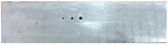
Figure 1.
The drawing of artificial defect test block.

Table 1.
Defect information.
All the inspections were performed with a 64-element ultrasonic array (Imasonic, Voray-sur-l’Ognon, France) with nominal center frequency of 5 MHz, (−6 dB bandwidth 86% of the center frequency), and a pitch of 0.6 mm, as well as a commercial array controller (Peak NDT LTPA, Derby, UK).
3. Methods and Results
3.1. TFM Imaging
Conventional ultrasonic phased array testing techniques utilize delay law to allow the firing of each transmitter in a pre-set sequence, whereby the beam into a test structure can be controlled to achieve translating, steering and focusing. As a consequence of a limited number of focal points, their imaging performance is significantly dependent on the distance from each focal point (i.e., the size of coverage area is proportional to the number of focal points, in this case) [14]. Furthermore, the efficacy of defect characterization is suppressed by measurable coherent noise arising from simultaneous firings of each aperture.
Drinkwater proposed an advanced imaging approach (known as TFM) using the so-called FMC data, whereby all the scattered signals from each transmit–receive pair are thoroughly exploited for post-processing [15]. The imaging resolution and detectability of TFM is overwhelmingly higher, relative to others [16,17]. The schematic diagram of transmission and reception in FMC is demonstrated in Figure 2 below.
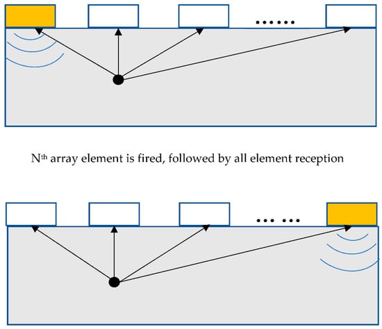
Figure 2.
Schematic diagram of FMC data acquisition.
Assuming htx,rx is the complex Hilbert transform of the time-domain received signals for each combination of transmitter (tx) and receiver (rx) elements in the FMC case, the intensity of the image, I(x, z), at any point in the image plane is, therefore, derived as:
where the location of imaging pixel is expressed with respect to x and z coordinates, c is the velocity of sound in the test structure and the summation is conducted over elements tx and elements rx. Note that linear interpolation is performed to select data from discrete time-domain signals [18,19]. Ultimately, the scattering information of each pixel can be maximumly extracted and imaged.
3.2. Image Data Augmentation
Insufficient practical samples of phased array imaging and high computational cost have led to a significant gap between effective defect classification and the use of deep learning algorithms. The data augmentation method utilizes auxiliary data sets or information to either enhance the features of samples in the target data or augment the size of target data sets, whereby the model can better extract features [20]. Prior study [21] also suggests that data enhancement might transform the original image data geometrically by changing the image pixel position with identical image features. Additionally, data enhancement methods, such as image rotation, change in image width and height, and image brightness modification [22], have been previously exploited to enlarge the plant image datasets of different defects with small samples, thereby solving the overfitting problem caused by the limited size of the dataset for machine learning. As shown in Figure 3, this study realized the novel augmentation of data sets by rotating the image, increasing noise and changing image brightness. Consequently, the augmented dataset, in which 25% of the image data was the test set and the remaining image data was the training set, is displayed in Figure 4 and Figure 5.
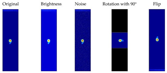
Figure 3.
Augmented dataset.
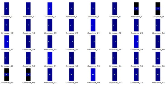
Figure 4.
SDH augmented dataset.
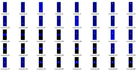
Figure 5.
Slot augmented dataset.
A sequence of experiments was performed to examine effectiveness of different image data augmentation techniques. The number of slot defects increased from 24 to 432, and the number of SDH defects increased from 8 to 144. The number of training and test sets before and after data expansion is given in the following Table 2 and Table 3.
Table 2.
Flaw wise augmented images for training.
Table 3.
Flaw wise augmented images for.
Furthermore, the HOG feature has been previously used to divide the image into small cells and obtain histogram description by gradient direction statistics inside each cell [23]. Its predominant purpose is to gray, normalize and calculate the gradient of the image, so as to extract the gradient information of the image [24]. In order to obtain contour and shape information of each image, the image pixel gradient is calculated by assuming the gray value of pixel (x,y) in the image as A(x,y), and, accordingly, the horizontal and vertical gradients of the pixel are expressed as follows:
The horizontal gradient of the pixel point is calculated as follows:
The pixel point direction gradient is calculated as follows:
The pixel point gradient amplitude is calculated as follows:
The pixel point gradient direction is calculated as follows:
As shown in Figure 6, the Hog feature of SDH defect was extracted.
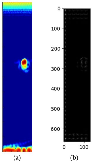
Figure 6.
(a) Original image; (b) HOG feature of TFM image.
3.3. SVM
SVM is a machine learning algorithm, based on statistical learning theory, which is of satisfactory learning performance in the case of small samples. As shown in the figure, SVM is a classification hyperplane that can distinguish positive samples from negative ones and maximize the interval between positive and negative samples in the high-dimensional feature space [25]. Linear SVM model is shown in Figure 7.
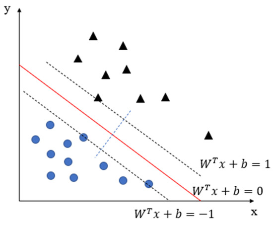
Figure 7.
Linear SVM model.
The SVM provides predicted solutions based on functional equation [26]:
Common SVM kernel functions include Linear kernel function, Polynomial kernel function, Gaussian kernel function and Sigmoid kernel function. The final classification result has a strong reliance on the type of SVM kernel function. In this paper, the accuracy rate was selected as the criteria. All the above-mentioned kernel functions were first compared for SVM image classification.
Unlike other approaches mentioned in this paper, the SVM utilizes a hinge loss function (HLF), in which the weights of irrelevant features are gradually reduced until they reach zero, and its classifier learns only a few points that are most relevant to classification. The HLF formula is given as follows:
The accuracy of HOG-SVM image classification under different kernel functions is shown in Figure 8.
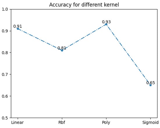
Figure 8.
Accuracy for different kernel.
As shown in Figure 8, HOG-Poly-SVM achieved the highest accuracy of 93% in realizing defect classification between SDHs and slots. Therefore, the kernel function of the SVM algorithm in this paper is thought to be a polynomial kernel function. In addition, the confusion matrix of classification results was performed to demonstrate the prediction accuracy of classification between SDH and slot details. According to the confusion matrix in Figure 9, when the HOG-Poly-SVM algorithm was used to predict and classify SDHs and slots in TFM images, the prediction accuracy of slot defects was 94% (i.e., 6% of slots were predicted as SDHs), and the prediction accuracy of SDH defects was 83% (i.e., 17% of SDHs were mispredicted to be slots).
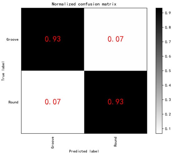
Figure 9.
SVM for Normalized confusion matrix.
3.4. CART Decision Tree
CART decision tree utilizes a greedy algorithm to select the optimum composition classification model from a large number of characteristics. The core idea of the CART decision tree algorithm is to recursively divide the samples into two samples by proposing the concept of dichotomy, and uses the Gini coefficient as the splitting point to measure the model’s impurity. Supposing there are M categories in the sample, and pm represents the probability of the m category, the Gini coefficient formula of the probability distribution of the sample points is written as follows [27]:
The classification of SDHs and slots realized in this article might be considered as a binary classification problem. Assuming P is the output probability of the first sample, the Gini coefficient of the probability distribution is:
Next, Hog was used to extract defect features, and the features were input into the Cart Decision tree algorithm (i.e., the HOG-CART Decision tree was exploited to predict and classify SDH and slots in TFM image), and the confusion matrix was obtained, as shown in Figure 10. Specifically, the prediction accuracy of slots was 91% and 9% of slots were mispredicted to be SDHs. The accuracy of SDHs was 77%, and 23% of SDHs were mispredicted to be slots.
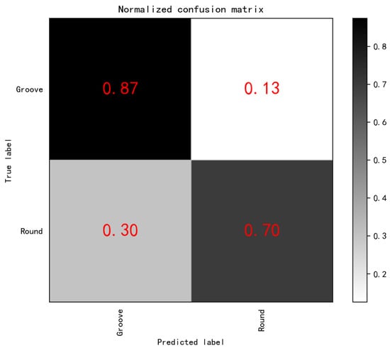
Figure 10.
Decision tree for Normalized confusion matrix.
3.5. KNN
KNN classification is a practically validated method to analyze parametric estimation of unknown probabilities [28]. The concept of the KNN algorithm is that first it identifies K training set samples with known category labels that are closest to, or most approximate to, unclassified sample X, and, then, it determines the category of sample X, according to the category labels of these K training samples. The distance between samples is measured by Euclidean distance, and the calculation formula is as follows [29]:
In an n-dimensional space, suppose the vector A is , the vector B is , then the formula for calculating the Euclidean distance of vector AB is:
Again, Hog was used to extract defect features, and the features were input into the KNN algorithm. The KNN algorithm K value in this paper was 11, that is to say, HOG-KNN was used to predict and classify SDHs and slots in TFM images, and the confusion matrix was obtained, as shown in Figure 11. The accuracy of slot defect prediction was 93%, with 7% of slot defects mispredicted to be SDH defects, and 50% of SDH defects were mispredicted to be slot defects.
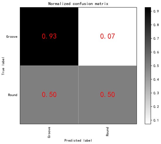
Figure 11.
KNN for Normalized confusion matrix.
3.6. Naive Bayes
The Naive Bayes classifier is a classification method based on conditional probability. Its principle is based on Bayes’ theorem, which is mainly used to predict the classification possibility of the unclassified data and to select the class with the highest probability as the final category of the sample [30]:
The probability of each sample category, yi, is calculated by the formula. Then, we count the probability of each sample belonging to each category and take the maximum value:
The category number with the highest probability, yk, is the characteristic of the final test sample.
Hog was also used to extract defect features, and the features were input into the Naive Bayes algorithm. The HOG–Naive Bayes Model was used to predict and classify SDH and slot defects in the TFM image, and the confusion matrix was obtained, as shown in Figure 12. The accuracy of slot defect prediction was 84%, with 16% of slot defects misinterpreted to be SDH defects. The accuracy of SDH defects was only 20%, and 80% of SDH defects were mispredicted to be slot defects.
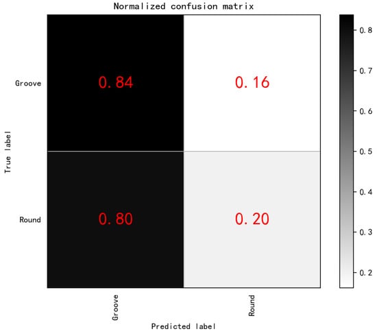
Figure 12.
Naive Bayes Model for Normalized confusion matrix.
4. Discussion
For binary classification problems, predicted results of classification are compared with those from true classification of the sample set, which can be summarized as the following four kinds of circumstances: (1) the model prediction is true and the real result is true (TP); (2) the model prediction is true and the real result false (FP); (3) the model prediction is false and the real result is true (TN); (4) the model prediction is false and the real result is false (FN). In this study, the accuracy rate, precision rate, recall rate and F1 function were employed to evaluate the advantages and disadvantages of the above four algorithms. Simultaneously, ten-fold cross-validation was conducted to evaluate the rationality of model selection.
Accuracy: The accuracy rate refers to the percentage of correct results in the total sample. The calculation formula is:
Precision: Precision is the proportion of samples that are predicted to be correct that are actually correct. The calculation formula is:
Recall rate: Recall rate is the proportion of actual positive samples that are predicted to be positive. The formula is as follows:
F1 score: This is an index to measure the accuracy of the binary classification model in statistics, and takes into account the accuracy rate and recall rate of the classification model. The formula is as follows:
As shown in Figure 13, for slot and SDH defects, the accuracy, recall and F1 function of the SVM algorithm outperformed those of the other algorithms. Thus, the preliminary results suggested that the SVM algorithm delivered a good classification effect in binary classification prediction of small-sample TFM images using ultrasonic phased array.
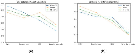
Figure 13.
(a) Slot data for different algorithms; (b) SDH data for different algorithms.
Figure 13 and Figure 14 clearly show the evaluation indices of slot and SDH defect prediction classification. In summary, the evaluation indices of the SVM algorithm were more advantageous, relative to those of other algorithms. Due to the small number of SDH samples, it was obvious, as can be seen in Figure 13 and Figure 14, that their predicted results were not as reliable as the predicted results from slot defect classification, which also indicated that the number of samples had significant influence on the predicted results of classification.
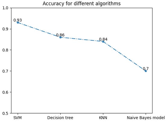
Figure 14.
Accuracy for different algorithms.
Meanwhile, for such small-sample data sets, the performance of the method using division of independent test sets was often not viable. This was because, in the case of small samples, it is necessary to select some test data which differ from the training set. Consequently, the scale of the training set becomes relatively small, leading to the problem of inadequate model training and overfitting. Ten-fold cross-validation divides the dataset into ten groups, nine of which are used as the training set and the remaining one as the test set. Each group of data is used as the test set in rotation with 10 cycles, as it is shown in Figure 15. By adopting the ten-fold cross-validation partition method, ten models, in which the evaluation results are calculated from the test set and their average value taken as the final result, are, therefore, obtained. This method can effectively use limited data to complete the training and evaluation of the machine learning algorithms, as shown schematically in Figure 16 below.
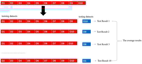
Figure 15.
Principle of ten-fold cross validation.
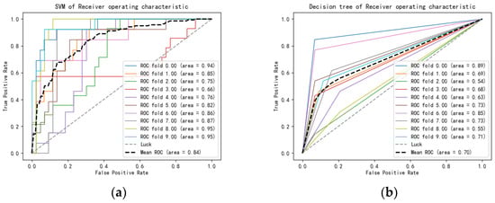
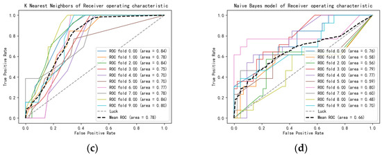
Figure 16.
(a) SVM of Receiver operating characteristic; (b) Decision tree of Receiver operating characteristic; (c) K Nearest Neighbors of Receiver operating characteristic; (d) Naive Bayes model of Receiver characteristic.
The above four algorithms were trained and evaluated by ten-fold cross-validation, and the receiver operating characteristic curve (ROC) drawn. The ROC curve describes the characteristics with respect to x-axis as False Positive rate and y-axis as True Positive rate. False Positive Rate and True Positive Rate can be calculated using the following formulae:
Since the better outcome was delivered by the higher True Positive rate and lower False Positive rate, the larger area under the ROC curve was preferred.
As presented in Figure 16a–d and Table 4, the SVM algorithm was seen to possess the largest average ROC area and provided the best prediction and classification effects of ultrasonic phased array TFM images, relative to the other three algorithms. This was consistent with the above evaluation results of accuracy rate, precision rate, recall rate and F1 score. Consequently, the SVM algorithm delivered satisfactory results in the classification of different defects, particularly in small-sample events found in ultrasonic phased array TFM images.
Table 4.
Comparison of performance metrics of different methods.
The TFM imaging of ultrasonic phased array could more accurately visualize the geometries of defects, relative to other approaches. Feature extraction in machine learning (e.g., extraction of shape features and HOG features) could be appropriately applied to TFM images, thereby realizing effective recognition of defects.
The typical characteristics of the TFM images include a small perceptual field of view and a large proportion of the background. For example, assuming the detection target is a small crack or a microscopic pore, the defect area represents a small proportion of the whole image, so that the local features dominate the final classification results. The SVM algorithm only learns a few points relevant to the classification criteria (i.e., pixels in vicinity of the defect). However, other algorithms described in this paper learn the average features of the background and defects, so that the relative weight of defect area in small object detection is reduced, leading to ineffective recognition. Consequently, the proper use of the SVM algorithm undoubtedly gives rise to the best solution for ultrasonic phased array TFM images.
5. Conclusions
From systematic study of the efficacy of off-the-shelf machine learning models using TFM images of typical defects found in pipelines, the CART decision tree algorithm uses the optimal features to partition each time. This greedy algorithm is dominated by the local optimum, which, thus, affects the final classification accuracy. The KNN algorithm relies strongly on the sample library and its similarity measure and distance function is not applicable. Furthermore, the KNN necessitates sufficient training samples to satisfy the relatively homogeneous feature space. This leads to measurable errors of image recognition under the conditions of small samples. In order to overcome such small-sample problems for industrial NDE, data augmentation is employed to increase the number of training samples. From our experiments, the results suggest that the KNN algorithm was inaccurate in predicting SDH defects, relative to slot-type defects, which could be attributed to an inability to solve sample imbalance (i.e., low prediction accuracy with a small number of samples). The Naive bayes approach requires an assumption of attribute feature independence, and classification of highly correlated data with attribute features makes it challenging to achieve an idealized effect. Moreover, the few training samples and uneven distribution of attribute features, give rise to significant errors relative to the actual test results. In this study, as a consequence of the small-sample problem with imaging results of SDHs and slots, the evaluation indices of the Naive Bayes algorithm in defect classification were found to be low, and, in particular, 80% of SDH defects were mispredicted as slot defects. Most notably, the SVM algorithm was developed to find a hyperplane category through the training data set. The classification results are predominantly determined by the sample categories of all the boundaries. The elimination of some samples does not directly affect the classification result. The ultrasonic phased array TFM images used in this study might be considered as a small-sample dataset for recognizing a small target. The SVM algorithm demonstrated its potential to resolve this problem. In comparison with other algorithms, the SVM also demonstrated promising classification results with the highest accuracy. The following conclusions may be drawn from the experimental results:
- (1)
- Pipeline safety is an important guarantee of energy security. In this paper, we proposed a machine learning algorithm for tube defect detection to improve the efficiency of defect detection for the purpose of ensuring energy security.
- (2)
- The effectiveness of four machine learning algorithms, applied to ultrasonic phased array TFM imaging, were compared, where the accuracy of the Naive Bayes model was 0.7, the accuracy of KNN was 0.84, the accuracy of decision tree was 0.86 and the accuracy of SVM was 0.93.
- (3)
- Ten-fold cross-validation was used to validate the four algorithmic models of classification effect. The SVM algorithm was significantly better than the other algorithms.
- (4)
- We first pointed out that the results of ultrasonic phased array TFM imaging are small object detection images.
- (5)
- In conclusion, we proposed a machine learning method for ultrasonic phased array TFM imaging, which could improve the efficiency of detecting defects. The highest accuracy, of 93%, could be achieved with this method. It provides ideas for future development of intelligent detection.
Therefore, the SVM algorithm is effective in the automated classification of defects, especially for small-sample events, such as TFM results, from energy pipelines.
This work only included two types of defects (SDH and angled slot), and it would be worth exploring the efficacy of the classification methods on more types of defects in future research. Furthermore, the data set used in this paper contained a small number of samples relative to the data sets used in other industries. In the future, simulation data might be supplemented to augment the machine learning data set by combining simulation data with experimental data. In comparison with traditional image classification methods, convolutional neural network is thought to yield a higher recognition rate and wider practicability. In conjunction with automated image feature extraction by convolutional neural network, the study of next-generation SVM has become one of the most fundamental research areas.
Author Contributions
Conceptualization, H.W.; Data curation, H.W., J.C. and W.C.; Formal analysis, W.C.; Funding acquisition, H.W.; Investigation, Z.F.; Methodology, X.C.; Resources, Y.B.; Validation, Z.W. All authors have read and agreed to the published version of the manuscript.
Funding
This research was funded by the National Key Research and Development Program of China (Project No. 2020YFB1506100), the National Natural Science Foundation of China (52202412), the Anhui Provincial Natural Science Foundation (2008085J24), and the Youth Science and Technology Foundation of Hefei General Machinery Research Institute (2022011502).
Conflicts of Interest
The authors declare no conflict of interest.
References
- Wasim, M.; Djukic, M.B. External corrosion of oil and gas pipelines: A review of failure mechanisms and predictive preventions. J. Nat. Gas Sci. Eng. 2022, 100, 104467. [Google Scholar] [CrossRef]
- Wasim, M.; Li, C.Q.; Robert, D.J.; Mahmoodian, M.; Setunge, S. Experiental investigation of factors influencing external corrosion of buried pipes. In Proceedings of the 4th International Conference on Sustainability Construction Materials and Technologies, Las Vegas, NV, USA, 7–11 August 2016. [Google Scholar]
- Huang, Y.; Zhong, S.; Fu, X.; Huang, X.; Tu, S. Ultrasonic phased array imaging and automatic identification of defects in polyethylene pipe electrofusion joints. Trans. China Weld. Inst. 2018, 39, 119–123. [Google Scholar]
- Zhang, X. The Study of Defect Map Processing and Intelligent Classification Technology in Ultrasonic Phased Array Exploration; Inner Mongolia University of Technology: Baotou, China, 2021. [Google Scholar]
- Sun, Y.; Sun, H.; Bai, P. Real-time automatic detection of weld defects in X-ray images. Trans. China Weld. Inst. 2004, 25, 115–118. [Google Scholar]
- Hou, W. Research on Defect Recognition of Weld Image Based on Deep Learning; University of Science and Technology of China: Hefei, China, 2019. [Google Scholar]
- Platt, J.C. Fast Training of Support Vector Machines Using Sequential Minimal Optimization; Advances in kernel methods; MIT Press: Cambridge, MA, USA, 1999; pp. 185–208. [Google Scholar]
- Zapata, J.; Vilar, R.; Ruiz, R. Automatic inspection system of welding radiographic images based on ANN under a regularization process. J. Nondestruct. Eval. 2012, 31, 34–45. [Google Scholar] [CrossRef]
- Barut, S.; Dominguez, N. NDT diagnosis automation: A key to efficient production in the aeronautic industry. In Proceedings of the 19th World Conference on Non-Destructive Testing [CP/DK], Munich, Germany, 13–17 June 2016. [Google Scholar]
- Wang, L. Image Recognition of Pressure Equipment Butt Weldings Using Ultrasonic Phased Array Inspection; Nan Chang Hang Kong University: Nanchang, China, 2014. [Google Scholar]
- Xie, Y.; Yang, T.; Lin, C. Research of Weld Defect Recognition in Flaw Detection through Ultrasonic Phased Array System. Chem. Eng. Mach. 2016, 43, 292–295. [Google Scholar]
- Pyle, R.J.; Bevan, R.L.T.; Hughes, R.R.; Rachev, R.K.; Ali, A.A.S.; Wilcox, P.D. Deep Learning for Ultrasonic Crack Characterization in NDE. Proc. IEEE Trans. Ultrason. Ferroelectr. Freq. Control 2021, 68, 1854–1865. [Google Scholar] [CrossRef] [PubMed]
- Bevan, R.L.T.; Croxford, A.J. Automated detection and characterization of defects from Multiview ultrasonic imaging. NDT Int. 2022, 128. in press. [Google Scholar] [CrossRef]
- Xue, W. Study on Realization and Denoising of Ultrasonic Phased Array Total Focusing Method Imaging; Southeast University: Nanjing, China, 2021. [Google Scholar]
- Holmes, C.; Drinkwater, B.W.; Wilcox, P.D. Advanced post-processing for scanned ultrasonic arrays: Application to defect detection and classification in non-destructive evaluation. Ultrasonics 2008, 48, 636–642. [Google Scholar] [CrossRef] [PubMed]
- Cheng, J.; Drinkwater, B.W.; Chen, X.; Fan, Z.; Chen, W.; Wang, Z. The pitch-catch nonlinear ultrasonic imaging techniques for structural health monitoring. Sci. China Technol. Sci. 2021, 64, 2608–2617. [Google Scholar] [CrossRef]
- Cheng, J.; Potter, J.N.; Drinkwater, B.W. The parallel-sequential field subtraction technique for coherent nonlinear ultrasonic imaging. Smart Mater. Strct. 2018, 27, 06500. [Google Scholar] [CrossRef]
- Cheng, J.; Potter, J.N.; Croxford, A.J.; Drinkwater, B.W. Monitoring fatigue crack growth using nonlinear ultrasonic phased array imaging. Smart Mater. Strct. 2017, 26, 055006. [Google Scholar] [CrossRef]
- Cheng, J. Measurement and Characterisation of a Diffuse Acoustic Field Using a Phased Array. Chin. J. Mech. Eng. 2021, 34, 129. [Google Scholar] [CrossRef]
- Zhao, K.; Ji, X.; Wang, Z. Survey on few-shot learning. J. Softw. 2021, 32, 349–369. [Google Scholar]
- Wang, H. Research on Few-Shot Image Recognition Technology Based on Data Augmentation and Metric Learning; University of Electronic Science and Technology of China: Chengdu, China, 2022. [Google Scholar]
- Gorad, B.J.; Kareppa, D.S. Novel Dataset Generation for Indian Brinjal Plant Using Image Data Augmentation. In IOP Conference Series: Materials Science and Engineering; IOP Publishing: Bristol, UK, 2021; Volume 1065. [Google Scholar]
- Huang, K.; Ren, W.; Tan, T. A Review on Image Object Classification and Detection. Chin. J. Comput. 2022, 37, 1225–1237. [Google Scholar]
- Wan, Y.; Li, H.; Wu, K.; Tong, H. Fusion with Layered Features of LBP and HOG for Face Recognition. J. Comput.-Aided Des. Comput. Graph. 2015, 27, 640–649. [Google Scholar]
- Meng, D. Research of Image Classification Methods Based on Deep Learning; East China Normal University: Wuhan, China, 2017. [Google Scholar]
- Singh, S.; Gupta, P. Comparative Study ID3, CART and C4.5 Decision Tree Algorithm: A Survey. Int. J. Adv. Inf. Sci. Technol. 2014, 27, 97–102. [Google Scholar]
- Adithya, T.; Chandramohan, D.; Sathish, T. Optimal prediction of process parameters by GWO-KNN in stirring-squeeze casting of AA2219 reinforced metal matrix composites. Mater. Today Proc. 2020, 21, 1000–1007. [Google Scholar] [CrossRef]
- Hu, J.; Fu, K. An Improved KNN Algorithm for Recognition of Handwritten Numerals. J. WUT (Inf. Manag. Eng.) 2019, 41, 22–26. [Google Scholar]
- Yang, T. Comparative study of traditional image classification and deep learning classification algorithms. J. Jing Chu Univ. Technol. 2020, 35, 27–34. [Google Scholar]
- Bao, Z. Research of Naïve Bayesian Image Classification Algorithm Based on Heterogeneous System Architecture; Beijing University of Technology: Beijing, China, 2017. [Google Scholar]


Publisher’s Note: MDPI stays neutral with regard to jurisdictional claims in published maps and institutional affiliations. |
© 2022 by the authors. Licensee MDPI, Basel, Switzerland. This article is an open access article distributed under the terms and conditions of the Creative Commons Attribution (CC BY) license (https://creativecommons.org/licenses/by/4.0/).