Abstract
In this article, an unsupervised learning method is presented with the objective of modeling, in real-time, the main operating modes (OM) of distribution transformers. This model is then used to assess the operational condition through use of two tools: the operation map and the health index. This approach allows, mainly, for a reduction in the need for the interpretation of results by specialists. The method used the concepts of k-nearest neighbors (k-NN) and Gaussian mixture model (GMM) clustering to identify and update the main OMs and characterize these through operating mode clusters (OMC). The evaluation of the method was performed using data from a case study of almost one year in duration, along with five in-service distribution transformers. The model was able to synthesize 11 magnitudes measured directly in the transformer into two latent variables using the principal component analysis technique, while preserving on average more than 86% of the information present. The operation map was able to categorize the transformer operation into previously parameterized levels (appropriate, precarious, critical) with errors below 0.26 of standard deviation. In addition, the health index opened the possibility of identifying and quantifying the main abnormal variations in the operating pattern of the transformers.
1. Introduction
Distribution transformers are present in large numbers on distribution grids, where it is common to find thousands of such devices in large urban centers. In addition, technologies related to the Internet of Things (IoT), edge computing and advanced metering infrastructure (AMI) have been combined to electric power systems, generating the so-called smart grids [1,2,3,4,5,6,7,8]. This combination allows, for example, the migration from the paradigm of preventative maintenance over to condition-based maintenance [9,10,11]. However, non-automated data collection and the need for specialists to interpret the results represent a significant limitation when applying diagnostic methods, on a large scale, to distribution transformers. As such, the development and improvement of methods that permit automatic diagnostic (i.e., capacity to determine the operational health status of these devices in an autonomous manner) can arrive at a significant contribution to the distribution sector of electric energy. Some of the main challenges associated with these automatic diagnostic methods are the ability to execute autonomously, use of algorithms that do not require human intervention or supervision, a simplified configuration with a minimum number of parameters that need to be estimated in advance, a structure that is adaptable and flexible to real-time measurements of the transformer and portability (i.e., applicability of the method independent of the transformer model or class).
In general, the automatic diagnostic methods are based on the concept of learning from the performance features over the long term, and in the identification of significant anomalous patterns that can lead to possible failure modes (set of operating patterns that the equipment presents when it fails). In addition, these techniques emphasize unsupervised learning algorithms, which can be online and real-time, to aid in decision-making and prognoses that autonomously identify tendencies that deviate from normal behavior, while also preventing possible failure states [12]. Deep learning, learning vector quantization, self-organizing maps and hidden Markov models are some of the tools typically used in automatic diagnostic methods [13]. However, the employment of such tools usually involves parameters as dissolved gas, short circuit impedance, frequency domain spectroscopy, humidity, etc. [14,15,16,17,18,19,20,21]. Therefore, the use of these parameters for distribution transformers can be very costly and inhibitory.
In this sense, this article discusses an unsupervised learning method, in real-time, that addresses some of the challenges cited, while proposing an automatic diagnostic strategy for distribution transformers. This new approach permits a system that executes this proposed method of automatic diagnostic to gradually tune the specifications of a particular transformer, through only its representation by a set of preselected feature variables (e.g., voltage, current, power factor, ambient temperature, tank temperature, total harmonic distortion.). Additionally, it provides the operator of the electric power distribution system, in graph form and without the need for deeper specific knowledge, information on the actual operational condition of the transformer. This reduces the need for detailed knowledge into the structural and dynamic properties of the transformer, together with its possible failure modes.
The proposed method includes two main tasks—basic modeling of the transformer in real-time and evaluation of the operational condition. The latter was implemented by means of two tools: the operation map and the health index. To this end, the method uses the concepts of clustering k-nearest neighbors (k-NN) and the Gaussian mixture model (GMM), for the automatic identification and updating of the main operational modes (set of stable patterns that the transformer presents in its various operating states) and establish the limits of the acceptable performance characteristics over the long term. The practical results presented in this study are based on a case study that has one year of data collected from five in-service distribution transformers.
The remainder of the article is organized in the following way. First, in Section 2, a description is given of the online data acquisition system, along with the magnitudes measured through it. Section 3 presents the automatic diagnostic method in real-time used to represent the data in a dynamic structure that models the transformer. Furthermore, it presents two tools, the operation map and the health index, which use this model to assess the condition of the transformer. Section 4 presents the results and the respective discussions of a case study based on the implementation of the method in a pilot set of five in service distribution transformers. The conclusions are given in Section 5.
2. Materials
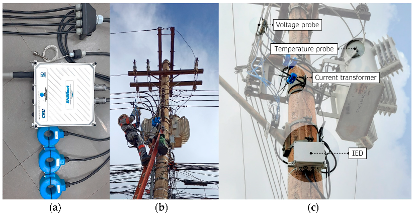
The proposed method is supplied with data collected in real-time from transformers on the distribution grid by a hardware device for wireless measurement and communication developed especially for this research. Figure 1 illustrates the hardware that is designated as IED (intelligent electronic device). The general specifications of the IEDs are presented in Table 1. Each of the IEDs were calibrated to the range specified in Table 1 using a programmable power source [22].
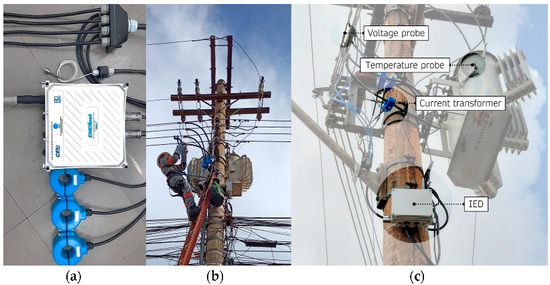
Figure 1.
Monitoring system of distribution transformers used to perform basic electrical and thermal measurements of the transformer. (a) IED (intelligent electronic device). (b) Non-intrusive installation process. (c) Distribution transformer real-time monitoring by the IED.

Table 1.
Specifications of IED.
The IED reads the sensors installed on the transformer at each second and then after three minutes, consolidates all the measurements and transmits the average values. These measurements are then used to produce the raw feature vector , where is the number of magnitudes measured on the transformer by the IED. In this study, and includes the measurements: electric voltages in per-unit (pu), currents in pu and power factor on each of the three phases (A, B, C) in low voltage; increase in tank temperature related to ambient temperature measured in loco and the total voltage harmonic distortion (THDv).
3. Automatic Diagnostic Method
The real-time automatic diagnostic method includes three main phases—(i) initialization, (ii) modeling and (iii) assessment of the condition. Figure 2 illustrates the main stages that make up the initialization and modeling phases, which are, respectively responsible for creating and updating a mathematical model of the distribution transformer. This model is then used in the condition assessment phase to evaluate the transformer. Prepensely, two tools are used, the operation map and the health index.

Figure 2.
Flowchart of the initialization and modeling phases of the real-time automatic diagnostic method.
3.1. Initialization Phase
In summary, the objective of the initialization phase is to standardize the raw features, reduce the dimensionality of the feature space, and identify stable patterns in the feature vectors that establish the different operational modes of the transformer. In this phase, one collects new raw feature vectors , until a predefined number, , necessary for the initialization, is reached. The minimum number of readings or data samples () is estimated from the number of independent parameters of the feature covariance matrix, which can be given by:
where is the number of magnitudes measured and indicates the dimension of .
As shown in Figure 2, the initialization phase is divided into three stages, standardization, dimensionality reduction and initialization of the model. All these stages are dealt with in the following section. The following notation will be used throughout this paper. The vectors and matrices are represented in boldface. The bar and tilde used over the symbols indicate the mean vector and the residual resulted of a process with information loss, such as principal component analysis (PCA).
3.1.1. Standardization
Once the initial set of raw feature vectors is complete and organized in the matrix , where each line represents a raw feature vector , these are standardized to guarantee that all the features are within the same magnitude. The mean of each feature is given in the vector
where . The raw feature vectors standardized to zero-mean and unit variance are given by
where
is the diagonal matrix for which the i-th element is the standard deviation of the i-th feature .
3.1.2. Dimensionality Reduction
In the following, the initial standardized feature vectors given by Equation (3) are transformed (projected) for the two-dimensional space, with the aim of eliminating redundant (correlated) features, allow a 2D visualization of key model steps, and alleviate known proximity issues when using Euclidean distance metrics in high-dimensional space [23]. The principal component analysis (PCA) technique was used to represent by means of its principal components , where is in addition to the total number of principal components, dimension of . From the properties of the Euclidean vector spaces and the PCA technique, one has that
where are the first two principal dominant components of , is the transformation matrix of the two first principal components. Analogously, and are, respectively the principal components and its respective transformation matrix. Moreover, as this study focused only on the two principal dominant components, it is called residual , the ignored contribution of the remaining principal components. In order to determine the transformation matrix, it is necessary, initially, to estimate the covariance matrix of the standardized features, in the following way:
Then, performing a singular value decomposition (SVD) [23] on the covariance matrix given by Equation (6)
one can determine the transformation matrix , composed of the first two columns of the square matrix . Through such, one obtains the first two dominant principal components of , which in the context of this study was denominated as operating points (OP), through the principal component (PC) transformation
3.1.3. Model Initialization
Now that the initialization dataset has been projected in the space of the two dominant principal components, generating the OPs, these are used to identify the initial operation modes (OM). The OMs are defined from the patterns formed by the OPs in the two-dimensional space of the two dominant principal components. The OMs are associated with different OPs but remain within the same envelope of operating conditions (e.g., overloaded, nominal operation, underutilized, etc.). Here, it was agreed that the OMs can be approximated by Gaussian probability distributions known as operating mode clusters (OMC). However, as these distributions are continuous, for the OMC to be fully characterized it is necessary to define an equiprobability boundary around each OMC. With this boundary, it is possible to determine whether an OP belongs to a given OMC. This boundary will be defined in Equation (23) of Section 3.2.3. Thus, it is said that the set of these clusters defines the OMC model. Figure 3 graphically illustrates these concepts.
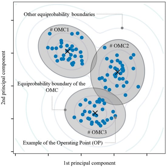
Figure 3.
Example of three patterns formed by OPs (operation modes) and approximated by three Gaussian distributions bounded by equiprobability boundaries (operation mode clusters).
The OPs generated in the previous dimensionality reduction stage were used to feed the Dirichlet process Gaussian mixture model [24]. Through use of this approach, one can identify with ease the clusters that correspond to the different OMs, where it is necessary only to indicate an upper limit for the number of OMs.
Accordingly, the following were determined: the number of initial OMCs , the respective centers and the covariance matrices . In addition to these parameters, that define the probability distribution associated with the OMC, two other parameters are initialized for each cluster—, which is the number of OPs that belong to each of the OMCs, and , which is the parameter that indicates the moment in which the i-th OMC was created. The difference , where is the number of the actual sample, defines the age of the i-th OMC. These two additional parameters are used later in Section 3.3.1 to calculate the health index of the transformer.
Since the initial OMs were approximated by gaussian probability distributions, the OMC model can be mathematically written as
where is the multivariate Gaussian probability distribution. The Dirichlet process is applied only during the initialization phase. Following this, in the modeling phase, the OMCs can update and increase in number, incorporating the potential new OMs.
3.2. Modeling Phase
Once the initialization phase is complete, and therefore an initial model of the transformer has been generated, the modeling phase can begin. This phase shares, with the initialization phase, the same flowchart in Figure 2. However, the modeling phase is implemented as a real-time unsupervised learning algorithm. In other words, it continually reads the new raw feature vectors, and dynamically updates the structure and parameters of the OMC model. In this way, the OMC model created in the initialization phase is always updated when a new data block is available.
As with the initialization phase, the modeling phase was similarly divided into three stages: recursive update of statistics (mean and standard deviation) and standardization process; recursive update of the transformation matrix to the space of the two dominant principal components and dimensionality reduction; and the learning process that consists of updating the OMCs to gradual changes in transformer dynamics or creating new OMCs when anomalous patterns are identified.
3.2.1. Standardization
This stage starts out by defining the matrix
as a set of all data blocks. Furthermore, the mean is related to through the following expression
Denoting , Equation (11) produces the following recursive calculation
The recursive calculation of is given by
where
Note that .
The recursive calculation of the standard deviation, derived in Appendix A, has the following relationship
where is the i-th column of the associated matrix, and are the i-th elements of the associated vectors.
Likewise, the recursive calculation of the covariance matrix, shown in Appendix B, has the following form
Older data can be skipped at an exponential rate, as it does not represent the current condition of the transformer. The recursive calculations for Equations (12), (15) and (16) with forgetting factor are
for . In the relationships above, is the forgetting factor. Low values of tend to forget old data more quickly, while
recover the case of not forgetting. The forgetting factor is a tuning parameter that varies depending on how quickly the normal process can change. The equation for this speed is described in Appendix C.
3.2.2. Dimensionality Reduction
The SVD transformation, Equation (7), of the updated covariance matrix determines the new transformation matrix . Allowing, as such, for the standardized feature vectors , calculated using Equations (14), (17) and (18), to be mapped for the space of the two dominant principal components following Equation (8), and resulting in OPs .
3.2.3. Learning Process
Let be the number of OMCs identified up to k-th iteration of the algorithm. A modified version of the k-NN algorithm is used to update the centers and the boundaries of the OMCs. First, the similarity between each, , where , and each one of the existing OMCs is assessed by verifying to the centers , of the existing OMCs. The metric used to calculate similarity was the Mahalanobis distance, given by Equation (21). This metric has as its main feature that it is appropriate for calculating the distance between two points in a probability distribution [25]. In addition, the Mahalanobis distance is scale invariant.
where . The shortest Mahalanobis distance determines the index of the closest (similar) OMC, that being
In order that the OP in fact belongs to the -th OMC it should be within the equiprobability boundary defined by
where is the chi-square distribution value with 2 degrees of freedom, and probabilistically defines the OMCs boundaries. When, for example, , one has , which corresponds to an equiprobability boundary of standard deviations.
If the OP under analysis is within the equiprobability boundary that limits the -th OMC, then it is used to update the OMC. As defined by Equation (9), for each OMC, there exists an associated Gaussian probability distribution. Therefore, to update the OMC signifies to update the mean and the covariance matrix of this distribution, as well as the age and the total number of OPs . Considering that the mean and variance do not have sudden changes between iterations, Equations (17) and (19) can be adapted for updating and , in the following manner
However, if the OP under analysis is outside the equiprobability boundary, Equation (23), then a new OMC is created to accommodate this new standard of operation
3.3. Operating Condition Assessment
3.3.1. Health Index
Each OMC, besides the associated Gaussian probability distribution, possesses two parameters: , which indicates the number of OPs that have already updated, and , which is the age of the OMC. These two parameters were inserted, as it is understood that these are important indicators as to the health of the transformer. An OMC that has most of the equipment operating time associated with it, that is, a large p value, is believed to be a healthier OMC. Similar to an OMC that was identified during the start of the operation of an admittedly healthy transformer. In other words, one expects that an old OMC is healthier than a new one. With the goal of joining, into one indicator, the parameters of age and number of OPs, one defines the health index () [14,26], which is calculated as follows
where is the total number of OMCs and .
The HI proposed in this study is a long-term trend indicator, and as such on the spot assessments may not be very indicative. For example, when a new OMC is created, it presents few OPs. This causes the HI, according to Equation (33), to enter a process of degradation of its value, as the transformer operation may, at times, be associated with this new OMC. However, if this new OMC continues to be populated by new OPs, or even, stops being populated, at some moment, the could reach an inflection point. From that point on, it gradually starts to increase. Faced with this behavior, it is interesting to determine whether the is still in the degradation stage or whether this process has already been overcome and, therefore, the is gradually returning to a healthy state. At a given instant for the moving average of the latter values of , it is said that the transformer is not in the degradation stage, when
where
3.3.2. Operation Map
This is a visual representation, in the space of the two dominant principal components of operation categories of the transformer. The categories are formed from intervals chosen for the feature variables, as in the example shown on Table 2, on which the operation of the transformer was divided into three categories (appropriate, precarious and critical). Since it is a categorization of the space itself of the two dominant principal components, the operation map must be restricted to a field of view and a precision, in order that it be implemented computationally. A field of view , with precision , is represented algebraically by the cartesian product
where and are intervals of the first and second principal components, respectively, which define the field of view. By applying the inverse PC transformation at any point at a given instant , one obtains
and following this by destandardizing , one has
One can, for example, categorize according to Table 2. When this process is repeated for every point , contiguous regions indicating the operation categories are formed. The flowchart in Figure 4 shows graphically the process of building the operation map. Colors can be used for a more intuitive representation of the operation categories. For example, green is appropriate, orange is Precarious, and red is critical.


Table 2.
Example of parameterization of the operation map.
Table 2.
Example of parameterization of the operation map.
| Operation Categories | Operation Map Restrictions | |
|---|---|---|
| Appropriate | 0.92 ≤≤ 1.05 and | ≤ 1.0 |
| Precarious | (0.87 ≤< 0.92) or (1.05 <≤ 1.06) or | 1.0 <≤ 1.2 |
| Critical | (< 0.87 or > 1.06) or | I > 1.2 |
1 Voltages in phases A, B and C given in pu. 2 Currents in phases A, B and C given in pu.

Figure 4.
Flowchart of the operation map construction process. The green circle represents that the region was classified as appropriate.
In this way, the operation map summarizes the set of rules defined in the space for the feature variables (Table 2 for example) in contiguous regions in the latent space of
where, according to the SVD transformation, Equation (7), is the diagonal matrix that contains the eigenvalues of .
Another important metric for measuring the performance of the operation map is the mean absolute error (MAE) of the PC transformation, given in numbers of standard deviation. Let any OP be , and the feature vector that originated it be , then the MAE of this OP, denoted as , is calculated in the following way
where is the dimensionality of , and is the residue of the PC transformation due to the suppression of the principal components.
In order to determine the error of each feature, in terms of its original magnitude, the absolute error (AE) was calculated for each destandardized feature. Let be the residual of . Therefore, the AE of each feature of an OP, denoted as , where i represents the i-th feature, is calculated as
where is the i-th value of , and is the standard deviation of the i-th feature as defined by Equation (4). The reconstruction errors given by Equations (40) and (41), cannot be extrapolated to the entire field of view .
4. Results and Discussion
The automatic diagnostics method proposed in this work was evaluated in a case study with five distribution transformers remotely monitored by the IEDs described in Section 2. The main construction and operational data of these distribution transformers are described on Table 3.

Table 3.
Main construction and operational data of the distribution transformers in the case study.
4.1. Initialization
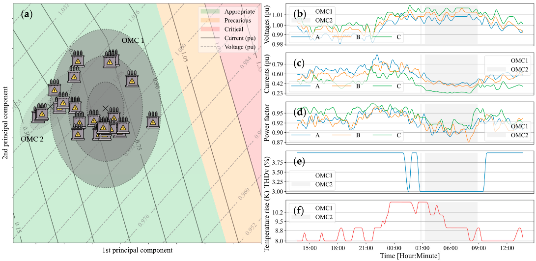
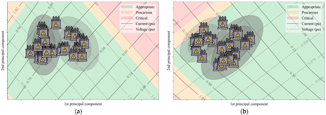
According to Equation (1), it is necessary to have, at least, independent feature vectors in order to commence the initialization phase. To avoid this obligation, the initial sample set was made up of raw feature vectors (i.e., covering the first day of monitoring of the transformer), thus making . Furthermore, considering a day means using the most relevant cyclic unit of transformer operation. This implies a greater stability of the model after initialization, since it is unlikely that there are relevant neglected operating patterns, thus preventing the model from going through major adaptations right from the start. Therefore, the initial set of each transformer in the case study can be submitted to the initialization phase described in Section 3.1. In this way, the initial OMC model for each transformer was built. For transformer 1, for example, the OPs for each hour of the first day of monitoring and the two OMCs found for approximating the operation modes are shown in Figure 5a. The set of measurements used in the initialization of the OMC model for transformer 1 are shown in Figure 5b. In addition, this figure indicates to which OMC each measurement belongs. This, therefore, indicates the OMC2 is associated, principally, to the period of 3 to 9 o’clock, where there exists a decrease in the current, which causes the transformer to cool down, the voltage to rise, and a decrease in the THDv. The remaining transformers were also initialized using two OMCs, as demonstrated in Figure 6a–d. Following a similar reasoning to transformer 1, the OMCs approximated the low- and high-load operating modes.
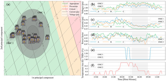
Figure 5.
Initialization of transformer 1. (a) Shows the initial OMCs and the OPs at each hour, as well as the operation map. (b–d) are the voltages and currents in pu, and the power factor of phases A, B and C. (e) is the total voltage harmonic distortion of the transformer. (f) is the temperature rise of the transformer tank in relation to the ambient temperature.
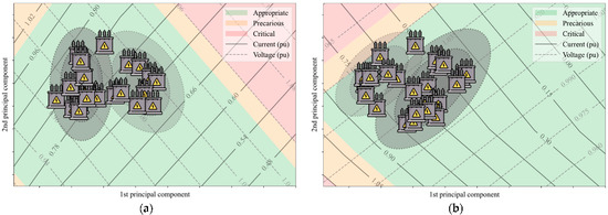
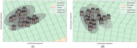
Figure 6.
Result from the initialization phase. (a–d) show the initial OCMs, the OPs for every hour, as well as the operation map of transformers 2, 3, 4 and 5, respectively.
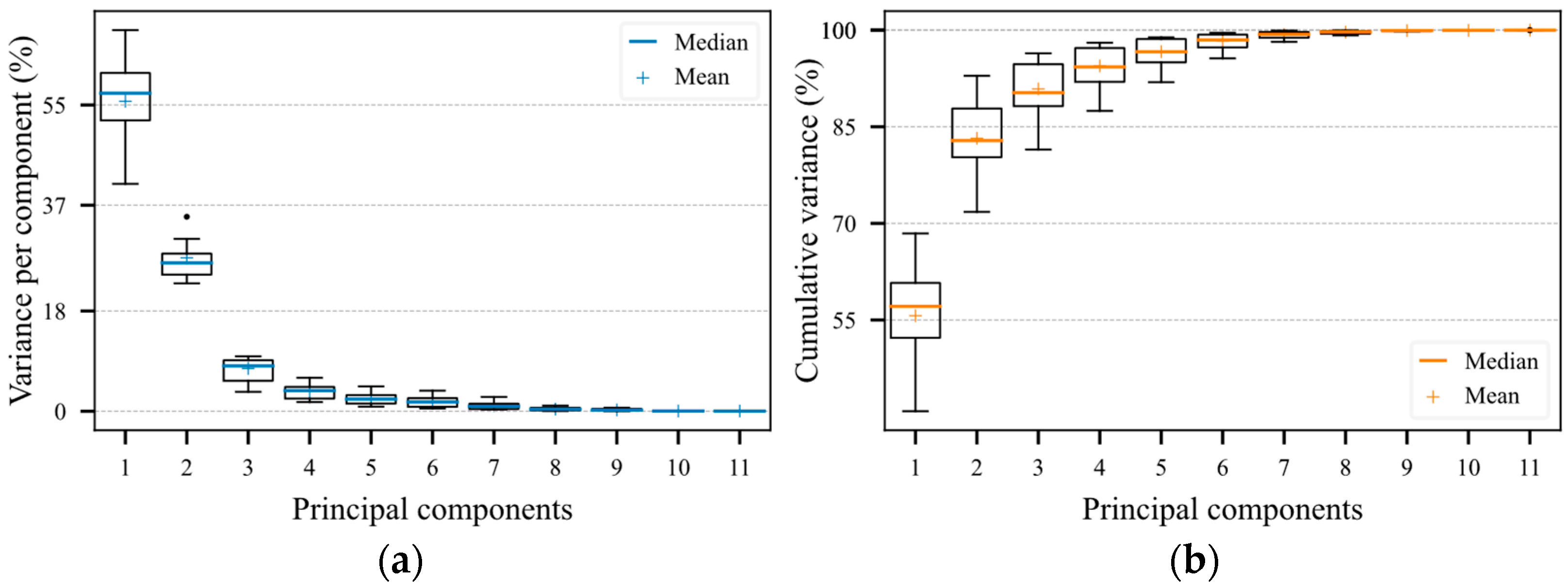
Figure 7a shows the distribution of the variance over the principal components of the five evaluated transformers, while Figure 7b shows the accumulated variance up to the respective principal component. Consequently, for the initialization data of the transformers, on average 83.32 ± 6.09% of the information (variance) was preserved using only the first two principal components. This result is important, as one of the premises of the method is the ability to synthesize measured data remotely, using the two dominant principal components. As such, only the two principal components represent more than 80% of the variation in the data.
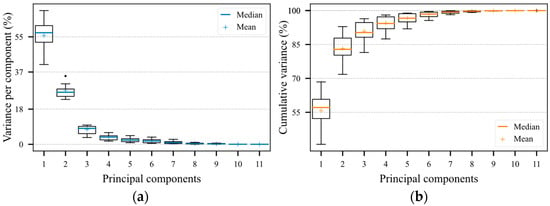
Figure 7.
Distribution of the variance of the five transformers on the principal components. (a) Variance on each component. (b) Accumulated variance up to the corresponding principal component.
4.2. Modeling
After the initialization phase, in which the dynamic base of operation of the transformers was identified, the modeling phase was started. In this phase, the automatic diagnostic algorithm is executed at each new feature vector. Therefore, the OMC model built in the initialization phase is updated both dynamically and autonomously. The only parameter that is configured manually is the rate of forgetting α. The tuning of this parameter took into account three aspects: importance of long-term evaluation, reconstruction error and variance preserved by the model.
For the important aspect of long-term evaluation, the value of α controls the weight given to a previous number of feature vectors. Low values of tend to forget old data more quickly. To adjust the rate of forgetting, besides considering an adequate sampling interval, it is also important that the variance preserved by the transformer OMC model , calculated by Equation (39), is elevated, and the reconstruction error , calculated by Equation (40), is as low as possible. Figure 8a shows the average for the quantity of variance preserved by the five models, regarding the rate of learning. This graph corroborates the choice of values for α getting closer to 1.

Figure 8.
Performance of the OMC model regarding the rate of forgetting (. (a) Accumulated variance up to the second principal component. (b) Reconstruction error given by Equation (40).
In contrast, the average reconstruction error, shown in Figure 8b demonstrates that values of α that tend to 1 generate increasingly larger errors. This is due to the fact that the model becomes increasingly slower in the identification of new standards, as α gets closer to 1. After all these considerations, a learning rate of was considered, which results in a weight of around 90% for the data gathered over the last 10 days of monitoring, calculated according to Equation C11. Therefore, an average reconstruction error of 0.16 ± 0.01 standard deviations and an average variance quantity of 80.22 ± 0.98% were expected, in accordance with the approximations shown in Figure 8a,b.
4.3. Operation Map
The operation map needs to be assessed, regarding the amount of variance that the OMC transformer model preserves, in terms of reconstruction error , calculated by Equations (39) and (40), respectively. If the error becomes large and/or the variance small, the operation maps lose their usefulness. As show in Figure 9, the average values in terms of the five transformers of the reconstruction error and the preserved variance remain considerably stable over the whole period of the case study. The highest average reconstruction error value encountered was 0.26 standard deviations, and the lowest preserved variance value was 86.12%.

Figure 9.
Average performance of the operation map regarding the five transformers. (a) Percentage of preserved variance and (b) Reconstruction error in number of standard deviations.
An elevated level of preserved variance does not necessarily generate a small reconstruction error. However, it is expected that a model that preserves a higher amount of variance has a lower reconstruction error. This point may be reinforced by the Pearson’s coefficient, which presented a correlation of 93.36 ± 0.01% between the reconstruction error and the quantity of variance preserved by the models.
The reconstruction error is an important measure of the general performance of the model. Therefore, to obtain a real dimension of the error, it is interesting to calculate the error of each feature individually. Figure 10a–e show the errors for each calculated feature, according to Equation (41). The highest error values encountered were 0.006 ± 0.009 (pu) for the voltages, 0.014 ± 0.008 (pu) for the currents, 0.004 ± 0.003 for the power factor, 6.56 ± 3.55% for the THDv and 0.272 ± 0.272 (K) for the rise in temperature.
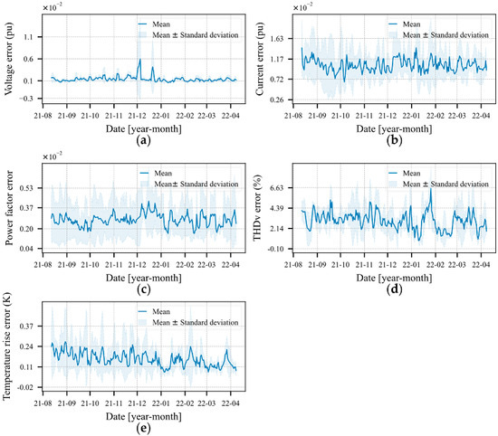
Figure 10.
Mean individual reconstruction error of the five transformers. (a) Sum of the errors over the three voltage phases. (b) Sum of the errors of the three phases over the currents. (c) Power factor (d) THDv. (e) Increase in tank temperature.
The results from the implementation of the operation map, using the parameterization of Table 2 and a precision of 0.05, are shown in Figure 5a and Figure 6a–d. Note the well-defined formation of the operation categories. A visual analysis of these regions in Figure 5a and Figure 6a–d indicates that all the transformers are operating appropriately and only transformer 3 is operating close to the precarious region, due to its voltage level.
4.4. Health Index
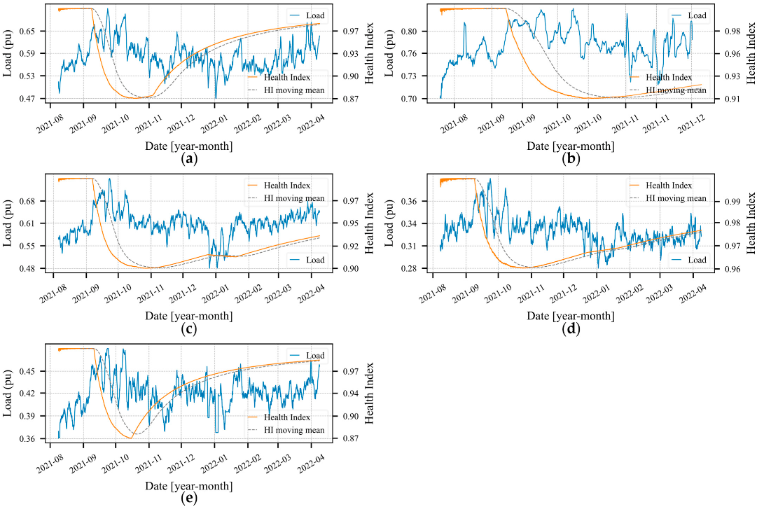
During the case study period, the method created OMCs to describe new modes of operation that were not described by the already existing OMCs. The creation of these new OMCs, initially with few OPs, led to the degradation of the HI. Noted here was that the creation of new OMCs was often related to changes in the loading pattern (average of currents on the three phases) of the transformer. Therefore, Figure 11a–e, demonstrate the daily loading average and the HI during part of the case study period. In addition, in this figure, the moving average of the HI is shown, which considers samples (i.e., 20 days). Through such, one reaches the conclusion that in all transformers, there are natural oscillations at the value of HI, since the condition imposed by Equation (34) was always satisfied after a given period.
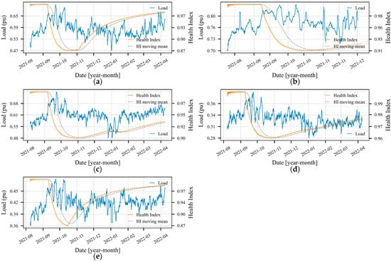
Figure 11.
Health index and loading of the transformer (sum of the currents for the three phases). (a–e) show the evolution of the HI during the case study, further highlighting the 20 days moving average of the HI.
The health index defined by Equation (33) has the advantage of not using as parameters measurements that are invasive and expensive, such as dissolved gas analysis [14,15], frequency response analysis [16,17,18], partial discharge analysis [19,20,21]. In addition, different to many of methods in current use of HI [14,26,27] eliminates the need to manually define the parameter weights.
4.5. General Considerations about the Case Study
Throughout the case study, the transformers were noted as operating for a greater part of the time within two OMCs. These two OMCs are predominantly associated with periods of lower and higher loads. However, as the transformers were not overloaded, there was not much permanence observed in the critical zone, except for occasions of grid events (such as overvoltages, for example).
Even though the initialization step (scheduled to take place on the first day of the start of monitoring) is responsible for defining the initial OMCs of the distribution transformer, variations in the transformer operation were observed when adapting these initial modes through the transformer adaptive model. Moreover, this is the very proposal of the transformer model, to identify new modes of operation at real-time.
Furthermore, in accordance with that indicated in Figure 6, each transformer has its own map representation for specific zones of operation (appropriate, precarious, etc.), which are allocated within different regions of the operational map. However, what is of importance to the user is the location of the OPs on the map in order to facilitate identification of their operation in real-time. In terms of how these fits into the reality of energy companies, this resource can contribute greatly when assessing their assets and their trends. The very proximity of the OPs in regard to critical or precarious regions, can be seen as an indication as to transformer operation tendency.
In some situations of this case study used to illustrate the proposed method, the formation of OPs in regions classified as “precarious” were noted. In practice, by analyzing the collected readings, grid phenomena were noted (such as overvoltage) that generated this operational change. Effects of cumulative damage need to be studied further, in order that they be incorporated into the HI. Even so, the proposal presented herein already demonstrates the capacity to produce an indicator that is adequate for the operation of a distribution transformer, while using only electrical parameters that are typically measured and above all, without the need for a specialist. Moreover, this is performed in real time and in autonomous fashion. Such resources as these, if applied on the scale of a distribution grid, can bring a series of insights that can be explored by the maintenance, power quality and network planning sectors of an energy company. In addition, with the quantity of data produced and information generated, it paves the way for the use of tools for data mining and artificial intelligence with the ability to evaluate the grid as a whole, potentially contributing to a more sophisticated scenario of smart grids.
5. Conclusions
In this article, an unsupervised learning method that models, in real-time, the main modes of operation (OM) of the distribution transformer were presented. The method used the concepts of k-nearest neighbors (k-NN) clustering and the Gaussian mixing model to identify the main OMs and characterize these as cluster of the operation mode (OMC). This model can be used to evaluate the operational condition of the distribution transformer, by means of two tools: the operation map and the health index.
The use of this unsupervised approach in real-time, allowed for the performing of the automatic diagnostic of the transformers, through a preselected set of feature variables. Thus, reducing the need for interpretation of results by experts. This is important, since with the advent of smart grids, the significant amount of data generated makes automatic diagnostic methods increasingly more necessary.
The assessment of the method was performed by means of data collected remotely and in real-time by a measurement IED. These data were collected over nearly one year, from five distribution transformers. The 11 magnitudes measured in the transformer were summarized in two latent variables (the two dominant principal components) preserving, during the case study, at least 86% of the information (variance). Additionally, the operation map was able to categorize the transformer operation with a low-level of reconstruction error, always below 0.26 standard deviations. Finally, the health index proved to be a viable automatic diagnostic index, permitting identification and quantification of abnormal variations in the operating pattern of the transformer.
Author Contributions
L.J.D.: conceptualization, methodology, Writing—original draft, investigation. A.P.P.: conceptualization, formal analysis, investigation. D.O.F.: writing—review and editing. All authors have read and agreed to the published version of the manuscript.
Funding
This research was funded, in part, by the R&D project 05160-1805/2018, granted by ANEEL and Neoenergia. The authors are also grateful to CNPq and UFU for additional funding.
Data Availability Statement
Data is available on request.
Conflicts of Interest
The authors declare no conflict of interest.
Appendix A
Following is the notations used in Section 3. All the data blocks, after having their averages calculated, can be described by
The standard deviation for the i-th variable is
and for the i-th standard deviation, we are led to
where two relationships, and have been applied.
Furthermore, consider the definition that
and we have Equation (15) instantaneously.
Appendix B
Substituting given by Equation (13) into the definition
directly yields
Using the fact that
in the above equation gives Equation (16) instantaneously.
Appendix C
The forgetting rate should reflect in a quantitative way the idea of adaptability to new patterns at the same time that old patterns are forgotten. The question of how long a feature vector will affect the recursive calculus depends on the magnitude of its composite variables and the learning rate. Concerning the magnitude, there is nothing that can be done; however, in the case of a real physical system; it is believed that there should not exist large variations (in the order of magnitude). Accordingly, it seems that the learning rate is responsible for determining how long a vector, with features of any type, will reverberate in the recursive calculation.
Therefore, simplifying the notation of Equation (17) for the recursive mean, but without loss of generality for the recursive variance and covariance equations. One has
By evaluating the previous iterations
and substituting Equation (A9) for Equation (A8), results in
By reorganizing Equation (A12), one obtains
There clearly emerges in Equation (A13) the pattern of a power series, which can more generally be written as
it becomes clear that the weight of the passed feature vectors is exponentially decreased. From Equation (A14), one can infer that the total weight given by all the previous feature vectors is
Yet, the weight omitted for stopping in the N-th feature vector is given by
The ratio between the total weight and the weight omitted demonstrates the percentage of weight that is given to the last vectors.
Thus, solving , one has
In order that the last feature vectors represent 90% of the weight, the learning rate should be in accordance with Equation (A18)
References
- Simoes, M.G.; Roche, R.; Kyriakides, E.; Suryanarayanan, S.; Blunier, B.; McBee, K.D.; Nguyen, P.H.; Ribeiro, P.F.; Miraoui, A. A Comparison of Smart Grid Technologies and Progresses in Europe and the U.S. IEEE Trans. Ind. Appl. 2012, 48, 1154–1162. [Google Scholar] [CrossRef]
- Dufour, C.; Bélanger, J. On the Use of Real-Time Simulation Technology in Smart Grid Research and Development. IEEE Trans. Ind. Appl. 2014, 50, 3963–3970. [Google Scholar] [CrossRef]
- Al Mhdawi, A.K.; Al-Raweshidy, H.S. A Smart Optimization of Fault Diagnosis in Electrical Grid Using Distributed Software-Defined IoT System. IEEE Syst. J. 2020, 14, 2780–2790. [Google Scholar] [CrossRef]
- Zhan, W.; Goulart, A.E.; Falahi, M.; Rondla, P. Development of a Low-Cost Self-Diagnostic Module for Oil-Immerse Forced-Air Cooling Transformers. IEEE Trans. Power Deliv. 2015, 30, 129–137. [Google Scholar] [CrossRef]
- Arritt, R.F.; Dugan, R.C. Distribution System Analysis and the Future Smart Grid. IEEE Trans. Ind. Appl. 2011, 47, 2343–2350. [Google Scholar] [CrossRef]
- Srivastava, I.; Bhat, S.; Vardhan, B.V.S.; Bokde, N.D. Fault Detection, Isolation and Service Restoration in Modern Power Distribution Systems: A Review. Energies 2022, 15, 7264. [Google Scholar] [CrossRef]
- Swain, A.; Abdellatif, E.; Mousa, A.; Pong, P.W.T. Sensor Technologies for Transmission and Distribution Systems: A Review of the Latest Developments. Energies 2022, 15, 7339. [Google Scholar] [CrossRef]
- Yang, W.; Chang, H.; Goudarzi, A.; Ghayoor, F.; Waseem, M.; Fahad, S.; Traore, I. A Survey on IoT-Enabled Smart Grids: Emerging, Applications, Challenges, and Outlook. Energies 2022, 15, 6984. [Google Scholar] [CrossRef]
- Jin, T.; Mechehoul, M. Minimize Production Loss in Device Testing via Condition-Based Equipment Maintenance. IEEE Trans. Autom. Sci. Eng. 2010, 7, 958–963. [Google Scholar] [CrossRef]
- Mariprasath, T.; Kirubakaran, V. A Real Time Study on Condition Monitoring of Distribution Transformer Using Thermal Imager. Infrared Phys. Technol. 2018, 90, 78–86. [Google Scholar] [CrossRef]
- Jardine, A.K.S.; Lin, D.; Banjevic, D. A Review on Machinery Diagnostics and Prognostics Implementing Condition-Based Maintenance. Mech. Syst. Signal. Process 2006, 20, 1483–1510. [Google Scholar] [CrossRef]
- Jaiswal, G.C.; Ballal, M.S.; Venikar, P.A.; Tutakne, D.R.; Suryawanshi, H.M. Genetic Algorithm–Based Health Index Determination of Distribution Transformer. Int. Trans. Electr. Energy Syst. 2018, 28, e2529. [Google Scholar] [CrossRef]
- Ochella, S.; Shafiee, M.; Dinmohammadi, F. Artificial Intelligence in Prognostics and Health Management of Engineering Systems. Eng. Appl. Artif. Intell. 2022, 108, 104552. [Google Scholar] [CrossRef]
- Rediansyah, D.; Prasojo, R.A.; Suwarno; Abu-Siada, A. Artificial Intelligence-Based Power Transformer Health Index for Handling Data Uncertainty. IEEE Access 2021, 9, 150637–150648. [Google Scholar] [CrossRef]
- Jiang, J.; Chen, R.; Chen, M.; Wang, W.; Zhang, C. Dynamic Fault Prediction of Power Transformers Based on Hidden Markov Model of Dissolved Gases Analysis. IEEE Trans. Power Deliv. 2019, 34, 1393–1400. [Google Scholar] [CrossRef]
- Chanane, A.; Houassine, H.; Bouchhida, O. Enhanced Modelling of the Transformer Winding High Frequency Parameters Identification from Measured Frequency Response Analysis. IET Gener. Transm. Distrib. 2019, 13, 1339–1345. [Google Scholar] [CrossRef]
- Abu-Siada, A.; Radwan, I.; Abdou, A.F. 3D Approach for Fault Identification within Power Transformers Using Frequency Response Analysis. IET Sci. Meas. Technol. 2019, 13, 903–911. [Google Scholar] [CrossRef]
- Miyazaki, S.; Tahir, M.; Tenbohlen, S. Detection and Quantitative Diagnosis of Axial Displacement of Transformer Winding by Frequency Response Analysis. IET Gener. Transm. Distrib. 2019, 13, 3493–3500. [Google Scholar] [CrossRef]
- Tozzi, M.; Saad, H.; Montanari, G.C.; Cavallini, A. Analysis on Partial Discharge Propagation and Detection in MV Power Transformers. In Proceedings of the 2009 IEEE Conference on Electrical Insulation and Dielectric Phenomena, Virginia Beach, VA, USA, 18–21 October 2009; pp. 360–363. [Google Scholar] [CrossRef]
- Firuzi, K.; Vakilian, M.; Darabad, V.P.; Phung, B.T.; Blackburn, T.R. A Novel Method for Differentiating and Clustering Multiple Partial Discharge Sources Using S Transform and Bag of Words Feature. IEEE Trans. Dielectr. Electr. Insul. 2017, 24, 3694–3702. [Google Scholar] [CrossRef]
- Nik Ali, N.H.; Giannakou, M.; Nimmo, R.D.; Lewin, P.L.; Rapisarda, P. Classification and Localisation of Multiple Partial Discharge Sources within a High Voltage Transformer Winding. In Proceedings of the 34th Electrical Insulation Conference, EIC 2016, Montreal, QC, Canada, 19–22 June 2016; pp. 519–522. [Google Scholar] [CrossRef]
- PW460 Protective Relay Test Kit Manufacturers, Suppliers, Factory, Company—PONOVO. Available online: https://www.ponovo.net/relay-and-protection-testing/protection-relay-testing-equipment-6i/pw460-protection-relay-test-set-is-the.html (accessed on 7 November 2022).
- Hashemipour, S.; Aghaei, J.; Kavousi-Fard, A.; Taher, N.; Salimi, L.; del Granado, P.C.; Shafie-Khah, M.; Wang, F.; Catalao, J.P.S. Optimal Singular Value Decomposition Based Big Data Compression Approach in Smart Grids. IEEE Trans. Ind. Appl. 2021, 57, 3296–3305. [Google Scholar] [CrossRef]
- Wang, B.; Li, Z.; Dai, Z.; Lawrence, N.; Yan, X. Data-Driven Mode Identification and Unsupervised Fault Detection for Nonlinear Multimode Processes. IEEE Trans. Industr. Inform. 2020, 16, 3651–3661. [Google Scholar] [CrossRef]
- Sarmadi, H.; Karamodin, A. A Novel Anomaly Detection Method Based on Adaptive Mahalanobis-Squared Distance and One-Class KNN Rule for Structural Health Monitoring under Environmental Effects. Mech. Syst. Signal. Process 2020, 140, 106495. [Google Scholar] [CrossRef]
- Ibrahim, K.; Sharkawy, R.M.; Temraz, H.K.; Salama, M.M.A. Selection Criteria for Oil Transformer Measurements to Calculate the Health Index. IEEE Trans. Dielectr. Electr. Insul. 2016, 23, 3397–3404. [Google Scholar] [CrossRef]
- Jaiswal, G.C.; Ballal, M.S.; Tutakne, D.R. Health Index Based Condition Monitoring of Distribution Transformer. In Proceedings of the IEEE International Conference on Power Electronics, Drives and Energy Systems (PEDES), Trivandrum, India, 14–17 December 2016; pp. 1–5. [Google Scholar] [CrossRef]
Publisher’s Note: MDPI stays neutral with regard to jurisdictional claims in published maps and institutional affiliations. |
© 2022 by the authors. Licensee MDPI, Basel, Switzerland. This article is an open access article distributed under the terms and conditions of the Creative Commons Attribution (CC BY) license (https://creativecommons.org/licenses/by/4.0/).

