Fault Diagnosis of Induction Motor Using D-Q Simplified Model and Parity Equations ^†

Abstract

Induction motors are the horsepower in the industrial environment, and among them, 3-phase induction motors (3PIMs) stand out for their robustness and standard 3-phase power supply. In the literature, there are many approaches to diagnose faults for the nonlinear 3PIM model, and the vast majority focus on a single motor fault, although others address more faults but at the cost of greater computational complexity. In this sense, one of the methods with less computational load and early detection is the parity equation approach, which is based on analyzing the discrepancy between the input and output signals of a real process and a linear mathematical model to generate a residual signal, which contains important information about the fault and is obtained through a suitable selection of a weighting matrix W to isolate the faults as much as possible. The problem in this case study is that the 3PIM model is a nonlinear system. In this work, the fault detection method based on the parity equations approach applied in the 3PIM is explored using a simplified and proposed model of the 3PIM working in the D-Q synchronous reference frame, which is matched with the direct current motor model to guarantee both the existence of the parity space and to ensure a large set of detectable faults in the 3PIM parameters. Simulation and experimental results validate the proposed scheme and confirm a very simple set of residual equations to guarantee both early detection and a large set of detectable faults in: Stator and rotor resistances, stator and rotor inductances, as well as current, voltage, and speed sensors. Additionally, development of human machine interface (HMI) is implemented to validate the proposed scheme.

1. Introduction

The induction motor (IM) is used in a wide variety of critical industrial applications where the principle of operation is based on reliable rotational motion, its reliability and service life can be increased through preventive/predictive maintenance schedules and with the help of a proper fault diagnosis system.

IMs are commonly subjected to external and extreme operating conditions, such as over temperature, unbalanced supply voltages, variable loads, and mechanical vibrations. All this causes changes in the IM parameter values and consequently causes a fault condition.

In a report on the reliability of IM in industrial processes [1], it was revealed that the rate of failure in the IM is approximately: 46% for stator, 26% for rotor (electrical failure), 11% for rolling bearings, and 17% for other components. In this sense, there is a growing interest in diagnosing faults for the IM [1,2], which can be used for maintenance schedules or for tolerant control.

According to stator faults, particularly stator winding faults and inter-turn short-circuit faults, many extensive and exclusive works have been found on a single fault with different approaches, such as the analysis by: Harmonic sequence current components analysis [3], operative condition monitoring [4], discriminant analysis using the D-Q synchronous frame [5,6], observer-based estimation [7], spectral analysis using vibration sensors [8], artificial intelligence using neuronal network [9,10], etc.

Regarding rotor faults, particularly by broken bar, many advanced studies with different methodologies have been extensively studied as the analysis by: Fault signature [11], motor current signature analysis [12], zero sequence current spectrum analysis [13], starting current analysis using optimized Stockwell transform [14], artificial intelligence analysis using neuronal networks [15,16], etc.

Related to mechanical faults in the IM rolling bearing, massive approaches have been harnessed to diagnose rolling bearing failure, some techniques used are based on thermal analysis [17], vibration analysis [18], measurement and analysis of external magnetic field [19], sound-acoustic emission analysis [2], artificial intelligence analysis using various estimation methods [16].

All the above research focused on the electrical and mechanical subsystems of the IM, such as failure in the stator winding, broken rotor bars, and degraded bearings, but the main issues of these types of techniques are: Large response delay time, high computational burden, large data storage, long detection and location time of the fault. Although for incipient faults the early detection delay time is not strongly necessary [20].

In order to diagnose early IM failure, model-based approaches are employed as the winding function approach [6], the parity equations approach [21], among others. The problem in [6] is that the model is simplified to the stator side of IM, and the drawback in [21] is that the direct current (DC) motor linear model is used, although a large number of electrical, mechanical, and magnetic parameters are obtained.

The main issue of model-based methods is the uncertainty of the model parameters and high sensitivity to noise, so this approach is commonly oriented to linear systems [21]. On the other hand, a nonlinear parity relation has been used to diagnose motor faults, particularly for faults in the resistances and inductances of the stator and rotor, which are indicative of faults such as overheating and short circuits in the winding [22]. However, the authors discretize and linearize the IM model equations, so the analytical approach is limited because the algebraic manipulation of its mathematical relationships is very long and complex. Therefore, the residual set is oriented to a reduced number of specific failures, and both the computational burden and the stored data are increased. Something similar happens when an artificial intelligence-based approach is used for IM fault detection, as in [16]. An advantage of the approach based on parity equations is the minimal mathematical complexity because the residual generation is analytical, and using fixed or adaptive thresholds, it is possible to detect multiple failures in the model parameters without using a data storage bank [23].

Operational conditional monitoring using mechanical and electrical signals is used to diagnose faults in [16] and [24], but the faults detected are generalized to failure over the stator, rotor, bearings, or misalignment, without identifying the damaged parameter associated with the IM. In this sense, detecting online a large number of IM model parameters using a single and easy-to-implement approach has not been widely addressed. On the other hand, some authors use simple and easy-to-implement methods in the IM as the average normalized current analysis [25] or the harmonic sequence analysis [3], but faults are only detected on the stator side.

Independent component analysis is a computational tool that allows statistically obtaining independent components of the system from electrical or mechanical signals. The approaches for this type of analysis are based on time-domain [26], frequency-domain [3], and hybrid algorithms [27]. The aforementioned strategies offer certain advantages, but the hybrid approach brings together a better performance in exchange for a higher computational burden, although some authors simplify it by concentrating on the feature knowledge of characteristic data on the stator side [28].

In the literature, there are some works that have considered various fault diagnostic methods applied to the IM in order to detect a certain number of electrical faults with a single approach. For example, in [10], a convolutional neural network is used and in [28], an analysis based on the knowledge of characteristics is used to detect failure in the rotor and bearings.

The problem remains that there are few efforts to detect parametric faults (faults in the 3PIM model internal parameters) and additive faults (faults in the 3PIM voltage and current sensors) using a single approach. The above is very important because all practical 3PIM faults are related to the electrical, magnetic, and mechanical parameters of the 3PIM model. For example, the stator winding faults, inter-turns short circuit, and broken bars in the rotor are a consequence of the variation or fault of the internal parameters of the 3PIM model, such as the resistances and inductances of the stator or rotor side, respectively, among others. In this sense, the techniques for parameter estimation, as in [7,29,30], are considered as a model-based fault detection approach. In [29], the case study focuses on a brushless DC motor and allows the identification of a large set of electrical, magnetic and mechanical parameters, however, the faults in the sensors and actuators are not obtained and a linear model is considered. Similarly, in [30], a large set of parameters is obtained through residual analysis but now using a nonlinear model, although the case studies are an evaporator system and a 4-tank system, and the residual programming is carried out for each parameter, which increases the computational effort. In [7], an observer-based estimation for the 3PIM is performed, although only the stator winding fault is analyzed. On the other hand, in [31], an online parameter identification method is presented using the PMSM linearized model using the D-Q system equations and taking into account nonlinear magnetic field. The drawback is that a fault detection system is not involved.

In [32,33], a fault detection scheme is carried out using the parity equations approach and the linearized 3PIM model through the D-Q synchronous reference frame. Then a large easy-to-implement residual set allows the detection of both electrical and mechanical parameters using a single approach. The problem encountered is that the residual weighting matrix W for residual generation is not very simplified, the implementation is not carried out, and some practical considerations are not taken into account.

In this paper, an extended and complementary scheme to improve the 3PIM fault detection system in [32,33] is proposed. The 3PIM model is more compressible and more simplified to obtain a linear model using some ideal electrical considerations in steady-state operation, such as the D-Q synchronous reference frame. Then, the diagnostic approach based on parity equations focused on fault detection in motor parameters and current, voltage, and speed sensors is performed using the linearized 3PIM model. This allows for a large set of detection parameters and eases implementation.

The organization of this work is as follows: The background of the parity equation method for fault detection and the analysis of the linearized 3-phase induction motor model for diagnosis are presented and developed in Section 2, respectively. The proposed fault detection for 3-phase induction motor using parity equation is described in Section 3. The simulation and experimental development are presented in Section 4 to validate the proposed method. Finally, in Section 5 the general conclusion of this work is expressed.

2. Motivation

As mentioned in the prior section, today, there are many well-known approaches to diagnosing faults in dynamic systems [34]. Regarding fault diagnosis applied to induction motors, a consensus opinion is high computational burden and high data storage capacity, even more so if the process is modeled without linearization and operating at variable speed. However, in many critical industrial applications with rotating machinery, it is only necessary to maintain a constant speed, such as ventilation, conveyor belts, electric cranes, etc., where online fault diagnosis in IMs is very useful either to plan corrective maintenance or to activate fault-tolerant mechanisms focused on the damaged parameter.

In this section, the well-known parity equations approach is shown with some practical considerations, then the linearized 3-phase IM model using the D-Q reference frame proposed in [32,33] and its similarity with the DC motor model is highlighted.

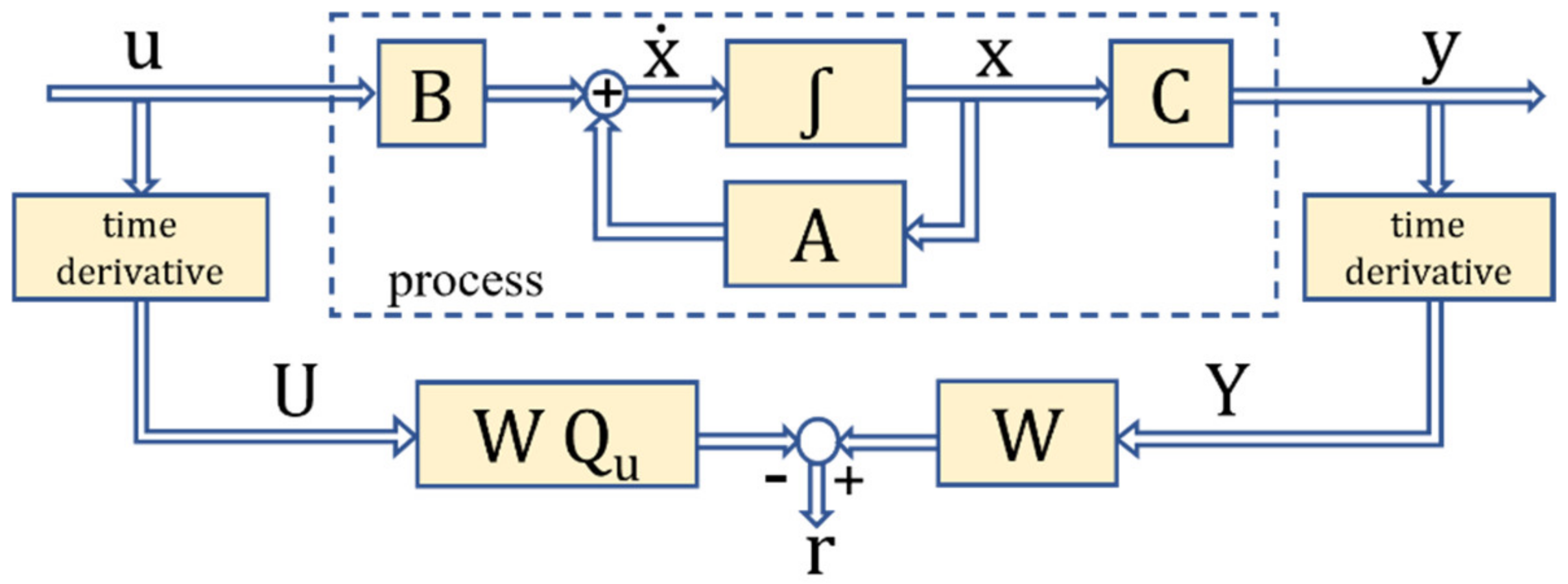
2.1. Parity Equation Method for Fault Detection

In general, a straightforward way to detect failures in a system is through residuals based on either process or signal modeling. These residuals are signals that compare the real-process and model behavior. Regarding the computational burden and from a practical point of view in linear systems, the parity equations scheme is a simple method to generate residuals, even than the observer-based approach [35].

A wide variety of approaches for fault diagnosis are available in the literature [4,36]. Most of these techniques are based on both continuous-time and discrete-time system models. However, in this case study, the attention is focused only on parity equations with state-space models for continuous-time, on this background, the parity equations residual design can be constructed with transfer functions or in state-space formulation, and the primary residuals that emanate from the output model or polynomial model do not necessarily allow to isolate faults. Nevertheless, the state space approach allows some freedom in the design of the weighting matrix W using two approaches for residual generation, which are structured design and directional design [20], the structured residual design means that the residuals must be decoupled from the faults to be detected, that is, the structured residual vector is at least independent of one of the faults. On the other hand, the directional residual design tries to reach a certain vector in the residual space for each fault, such that the direction is fixed, but the length of the vector depends on the fault size [34].

The linear parity equations, widely studied in the literature, as in [20,34], are commonly developed from the continuous-time state-space model with multi-input multi-output and are given by

$$\dot{x}\left(t\right)=A\mathrm{x}\left(t\right)+B\mathrm{u}\left(t\right)+V\mathrm{v}\left(t\right)+L{\mathrm{f}}_l\left(t\right)$$

(1)

$$y\left(t\right)=C\mathrm{x}\left(t\right)+N\mathrm{n}\left(t\right)+M{\mathrm{f}}_m\left(t\right)$$

(2)

where, $\mathrm{x}\left(t\right)$, $\mathrm{u}\left(t\right)$, $\mathrm{v}\left(t\right)$, ${\mathrm{f}}_l\left(t\right)$, $\mathrm{n}\left(t\right)$, and ${\mathrm{f}}_m\left(t\right)$ are state, input, input-noise, input-fault, output-disturbance, and output-fault vectors, respectively. A, B, V, L, N, and M are their corresponding matrices. Moreover, C is output matrix.

Then taking into account only processes with negligible signals of noise-disturbance and additive-faults, we have that the first and second derivate of y(t) are:

$$\dot{y}\left(t\right)=CA\mathrm{x}\left(t\right)+CB\mathrm{u}\left(t\right)$$

(3)

$$\ddot{y}\left(t\right)=C{A}^2\mathrm{x}\left(t\right)+CAB\mathrm{u}\left(t\right)+CB\dot{\mathrm{u}}\left(t\right)$$

(4)

In this way, each time the number of derivatives increases, a redundancy is generated as long as q ≤ n where q is input number, and n is the order of system, which leads to a system of equations as in [34]:

$$Y\left(t\right)=T\mathrm{x}\left(t\right)+Q_{u}U\left(t\right)$$

(5)

with

$$\begin{gathered} Y\left(t\right)=\left[\begin{array}{c}y\left(t\right)\\ \dot{y}\left(t\right)\\ \begin{array}{c}⋮\\ y^{\left(q\right)}\left(t\right)\end{array}\end{array}\right] U\left(t\right)=\left[\begin{array}{c}u\left(t\right)\\ \dot{u}\left(t\right)\\ \begin{array}{c}⋮\\ u^{\left(q\right)}\left(t\right)\end{array}\end{array}\right] T=\left[\begin{array}{c}C\\ \begin{array}{c}CA\\ C{A}^2\end{array}\\ \begin{array}{c}⋮\\ C{A}^q\end{array}\end{array}\right] \\ {Q}_u=\left[\begin{array}{ccc}\begin{array}{ccc}\begin{array}{c}0\\ CB\\ CAB \end{array}& \begin{array}{c}0\\ 0\\ CB\end{array}& \begin{array}{c}0\\ 0\\ 0\end{array}\end{array}& \begin{array}{c}\cdots \\ \dots \\ \cdots \end{array}& \begin{array}{c}0\\ 0\\ 0\end{array}\\ \begin{array}{cc}⋮ ⋮ & ⋮\end{array}& \ddots & ⋮\\ \begin{array}{ccc}C{A}^{q-1}B& C{A}^{q-2}B& \dots \end{array}& CB& 0\end{array}\right] \end{gathered}$$

(6)

For a system of order n with q inputs and r outputs the following matrices have the following orders:

• $Y\left(t\right)$ is a vector $\left(q+1\right)r\times 1$
• $U\left(t\right)$ is a vector $\left(q+1\right)p\times 1$
• $T$ is a matrix $\left(q+1\right)r\times n$

Multiplying (5) by a vector $W^T$ in both sides:

$$W^{T}Y\left(\mathrm{t}\right)=W^{T}T \mathrm{x}\left(t\right)+W^T{Q}_{u}U\left(t\right)$$

(7)

By selecting $W^T$ with dimension $\left(1\times \left(q+1\right)r\right)$ and with a condition such that:

$$W^{T}T=0$$

(8)

Then a residual vector r(t) equal to zero is obtained in a fault-free condition, such that

$$r\left(t\right)=W^{T}Y\left(t\right)-W^T{Q}_{u}U\left(t\right)$$

(9)

More residual terms are found added more different vectors $W^T$, so creating a matrix $W$ and the residual vector, at last, becomes

$$r\left(t\right)=WY\left(t\right)-W{Q}_{u}U\left(t\right)$$

(10)

where the dimension of $W$ determines the number of residues in the parity equation. Figure 1 shows the simple scheme of parity equations without noise-disturbance and additive-fault signals.

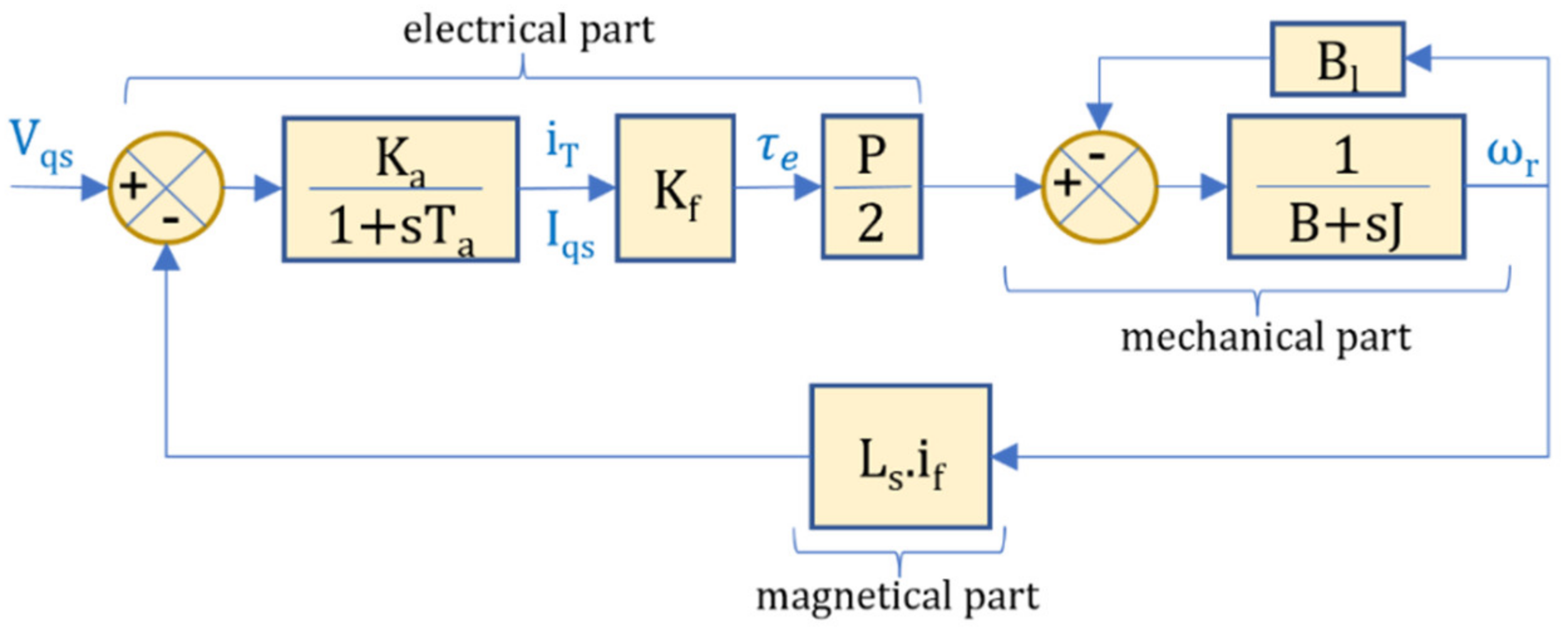
2.2. Linearized 3-Phase Induction Motor Model

The goal of this section is to find a 3-phase induction motor (3PIM) state spaces model that can be used to diagnose faults using the parity equations approach described in the previous section, the starting point to carry out is to consider the synchronous reference frame theory and the steady-state behavior [37,38] to identify the 3PIM subsystems related to the mechanical, electrical, and magnetic parts. The main idea is to analytically match the 3PIM model with the DC motor model and find the definition of its parameters to define the state space equation for fault diagnosis.

The 3PIM stator equations under the synchronous reference frame are

$$V_{qs}{}^e=\left(R_s+L_s\rho \right)i_{qs}{}^e+{\omega }_s{L}_s{i}_{ds}{}^e+L_m\rho i_{qr}{}^e+{\omega }_s{L}_m{i}_{dr}{}^e$$

(11)

$$V_{ds}{}^e=\left(R_s+L_s\rho \right)i_{ds}{}^e-{\omega }_s{L}_s{i}_{qs}{}^e+L_m\rho i_{dr}{}^e-{\omega }_s{L}_m{i}_{qr}{}^e$$

(12)

where $V_{qs}{}^e$, $V_{ds}{}^e$, $i_{qs}{}^e$, and $i_{ds}{}^e$ are the voltages and currents of stator in the D-Q synchronous reference frame, respectively. $R_s$ and $L_s$ are the symmetrical matrices of stator resistances and inductor, respectively. $i_{qr}{}^e$ and $i_{dr}{}^e$ are the rotor current in the D-Q synchronous reference frame, respectively. $L_m$ and ${\omega }_s$ are the magnetizing inductance and stator angular speed, respectively.

The key assumption is that the rotor flux link ${\Psi }_r$ is constant, so its derivatives are zero. The 3PIM steady-state analysis allows identifying the blocks of the transfer function, which can be divided into electrical, mechanical, and magnetic parts.

Some rotor-side equations are considered as the relationships of the d-q-axis flux linkages for recast the stator voltage equations as follows, where $L_r$ is the rotor inductance matrix. For convenience in syntax, the superscript of the currents and voltages d-q are dropped.

$$i_{qr}=-\frac{L_m}{L_r}{i}_{qs}$$

(13)

$$i_{dr}=\frac{{\Psi }_r}{L_r}-\frac{L_m}{L_r}{i}_{ds}$$

(14)

Substitution of (13) and (14) into the stator-voltage (11) and (12) results in

$$V_{qs}=\left(R_s+\sigma L_s\rho \right)i_{qs}+\sigma {\omega }_s{L}_s{i}_{ds}+{\omega }_s\frac{L_m}{L_r}{\Psi }_r$$

(15)

$$V_{ds}=\left(R_s+\sigma L_s\rho \right)i_{ds}-\sigma {\omega }_s{L}_s{i}_{ds}+\frac{L_m}{L_r}\rho {\Psi }_r$$

(16)

where σ is the leakage coefficient, $\rho$ is the derivative operator, $L_r$ is rotor inductance matrix, but according to the 3PIM steady-state behavior, the stator current flux-producing component $i_f$ is constant, and that is the stator d-axis current $i_{ds}$ in the synchronous reference frame. Its derivatives are also zero

$$i_f=i_{ds}$$

(17)

$$p{i}_{ds}=0$$

(18)

Likewise, the stator current torque-production component $i_T$ is the stator q-axis current $i_{qs}$ and the rotor flow linkage ${\Psi }_r$ is defined as follows

$$i_T=i_{qs}$$

(19)

$${\Psi }_r=L_m{i}_f$$

(20)

Now, substituting (17)–(19) into (15)

$$V_{qs}=\left(R_s+L_a\rho \right)i_T+{\omega }_s{L}_a{i}_f+{\omega }_s\frac{L_m{}^2}{L_r}{i}_f=\left(R_s+L_a\rho \right)i_T+{\omega }_s{L}_s{i}_f$$

(21)

with

$$L_a=\sigma L_s$$

$$L_s=L_a+\frac{L_m{}^2}{L_r}$$

The second stator Equation (16) is not required, the solution of either will yield $i_T$, now, the stator frequency is represented as

$${\omega }_s={\omega }_r+{\omega }_{s1}={\omega }_r+\frac{i_T}{i_f}\left(\frac{R_r}{L_r}\right)$$

(22)

The electrical part equation of the motor is obtained by substituting for ${\omega }_s$ from (22) into (21) so

$$V_{qs}=\left(R_s+\frac{R_r{L}_s}{L_r}+L_a\rho \right)i_T+{\omega }_r{L}_s{i}_f$$

(23)

From which the stator current torque-producing component is derived as

$$I_T=\frac{V_{qs}-{\omega }_r{L}_s{i}_f}{R_s+\frac{R_r{L}_s}{L_r}+L_a\rho }=\frac{K_a}{1+s{T}_a}\left(V_{qs}-{\omega }_r{L}_s{i}_f\right)$$

(24)

with

$$R_a=R_s+\frac{L_s}{L_r}{R}_r$$

$$K_a=\frac{1}{R_a}$$

$$T_a=\frac{L_a}{R_a}$$

From this block, the electromagnetic torque ${\tau }_e$ is written through voltage and speed feedback into the torque current as follows

$${\tau }_e=K_f{i}_T$$

(25)

with

$$K_f=\frac{3}{2}\frac{P}{2}\frac{L_m{}^2}{L_r}{i}_f$$

For the mechanical part, the dynamic loads can be represented, taking into account both the electromagnetic torque and the load torque, which is considered friction in this particular case.

$$J\frac{d}{dt}\left({\omega }_r\right)+B{\omega }_m={\tau }_e-{\tau }_L=K_f{i}_T-B_l{\omega }_m$$

(26)

In terms of the rotor electrical speed ${\omega }_r$, it is derived by multiplying both sides by the pair of poles.

$$J\frac{d}{dt}\left({\omega }_r\right)+B{\omega }_r=\frac{P}{2}{K}_f{i}_T-B_l{\omega }_r$$

(27)

Finally, using (24), (25), and (27), a block diagram of the 3PIM model is obtained, which is matched with the DC motor model, as shown in Figure 2.

Then, in the same way, as in the DC motor model, the input/output variables for the 3PIM model are $V_{qs}$, $I_{qs}$ and ${\omega }_r,$ respectively, as follows

$${\dot{\mathrm{I}}}_{qs}=\frac{-R_a{I}_{qs}}{L_a}-\frac{L_s{i}_f{\omega }_r}{L_a}+\frac{V_{qs}}{L_a}$$

(28)

$${\dot{\omega }}_r=\frac{(K_f{N}_p)I_{qs}}{J}-\frac{\left(B_l+B\right){\omega }_r}{J}$$

(29)

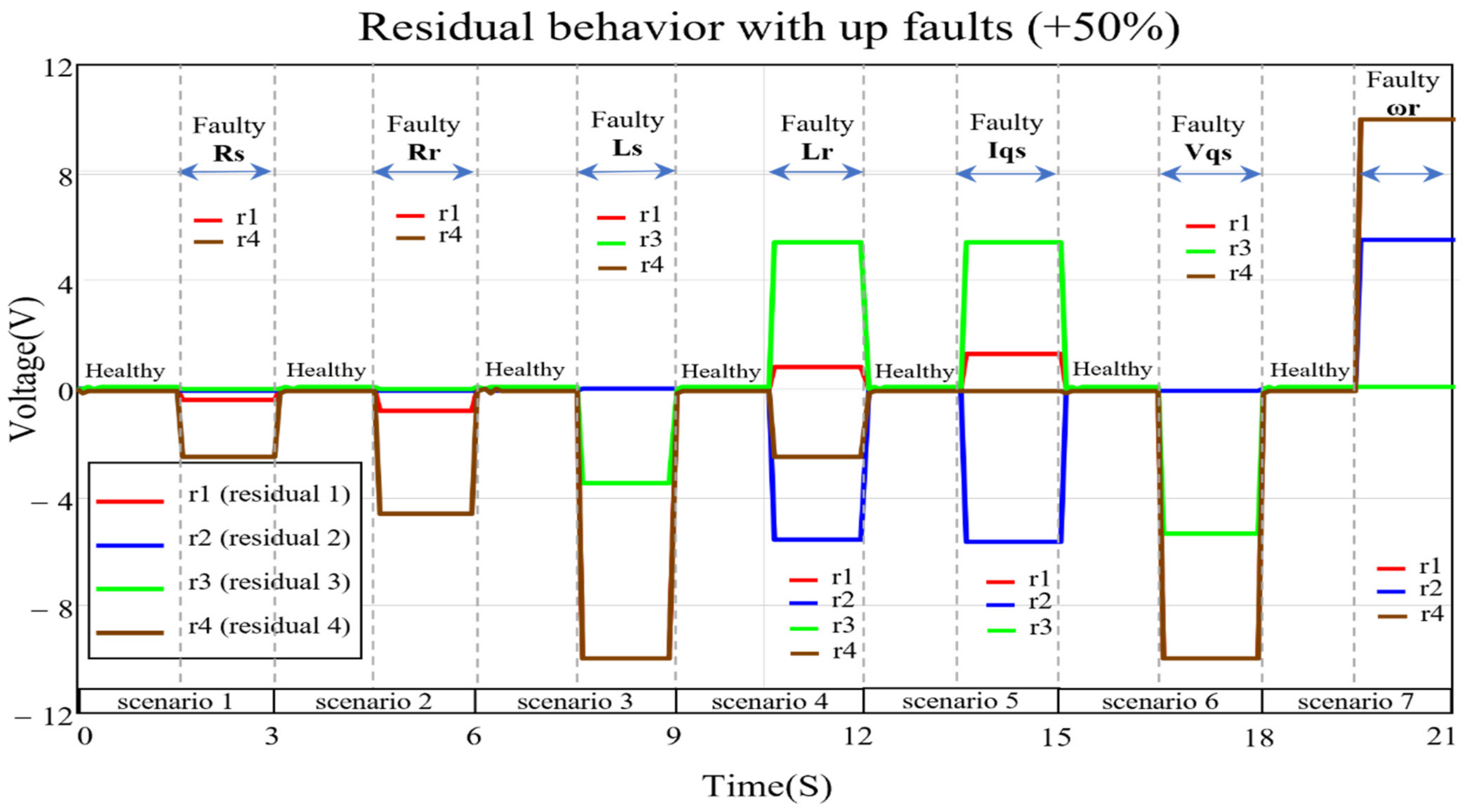
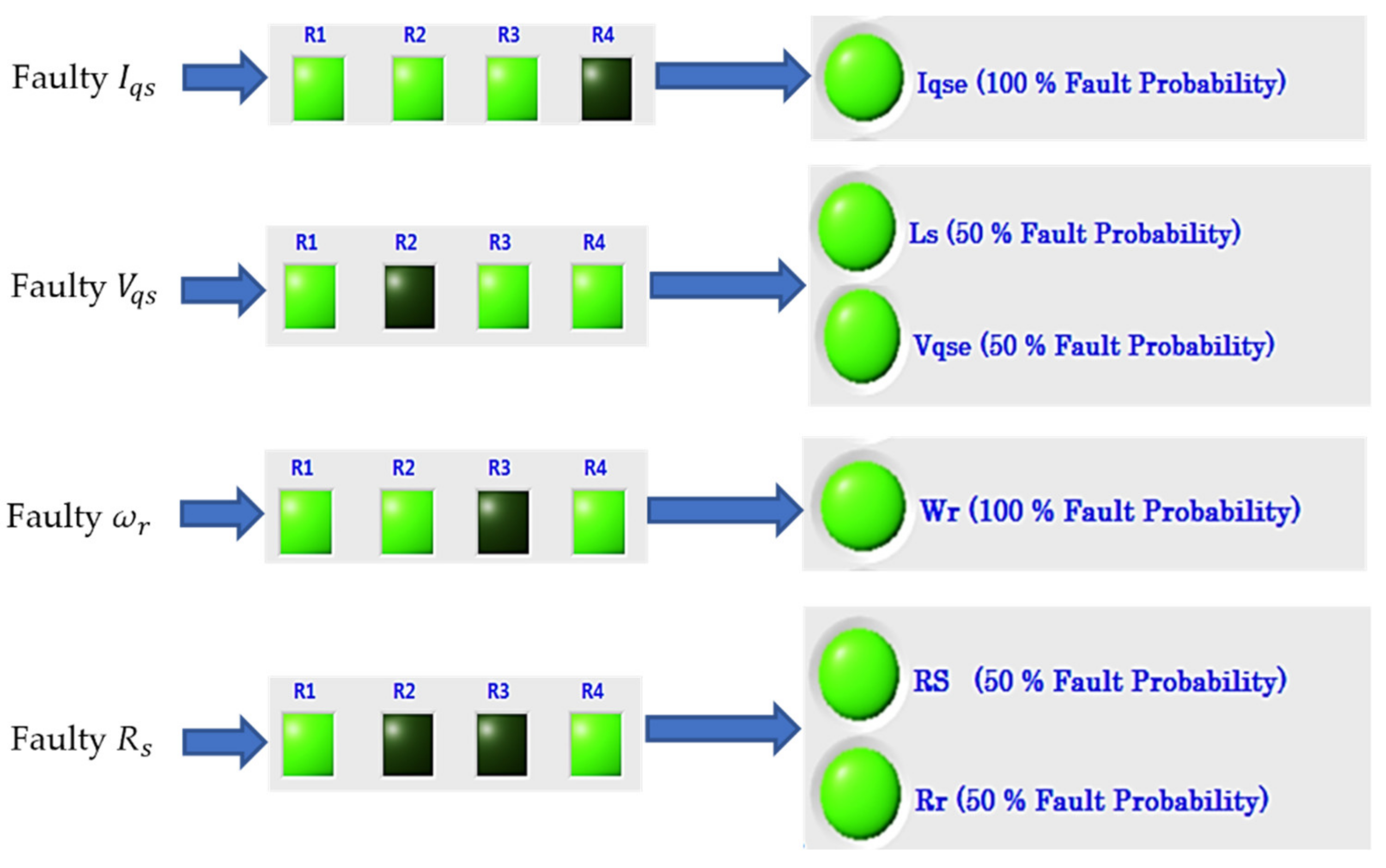
3. Fault Detection for 3-Phase Induction Motor Using Parity Equation

Regarding the coupling of the mechanical, electrical, and magnetic parts of the 3PIM, the transfer function considers a link that relates the current that produces the torque and the induced magnetic force, this link is a 3PMI total current loop and is independent of the mechanical system [38]. This model is like the DC motor model obtained in [39]. Although the difference is that the input signal is $V_{qs}$ instead of the armature voltage. In this way, the 3PIM model based on D-Q reference frame obtained in the previous section is given by

$$\dot{x}\left(t\right)=\mathit{A}x\left(t\right)+\mathit{B}u\left(t\right)$$

(30)

$$y\left(t\right)=\mathit{C}x\left(t\right)$$

(31)

$$x\left(t\right)=\left[\begin{array}{c}{I}_{qs}\\ {\omega }_r\end{array}\right] u\left(t\right)=\left[\begin{array}{c}{V}_{qs}\\ 0\end{array}\right] \dot{x}\left(t\right)=\left[\begin{array}{c}{\dot{I}}_{qs}\\ {\dot{\omega }}_r\end{array}\right] y\left(t\right)=\left[\begin{array}{c}{I}_{qs}\\ {\omega }_r\end{array}\right]$$

(32)

$$\mathit{A}=\left[\begin{array}{cc}\frac{-R_a}{L_a}& -\frac{L_s{i}_f}{L_a}\\ \frac{K_f{N}_p}{J}& \frac{-\left(B_l+B\right)}{J}\end{array}\right] \mathit{B}=\left[\begin{array}{cc}\frac{1}{L_a}& 0\\ 0& 0\end{array}\right] \mathit{C}=\left[\begin{array}{cc}1& 0\\ 0& 1\end{array}\right]$$

(33)

Substituting the previous matrices in (6), a pair of matrices T and ${\mathit{Q}}_u$ are obtained, then the output function $Y\left(t\right)$ in (5) is derived but without disturbances and without external faults $V\left(t\right)=N\left(t\right)=F\left(t\right)=0$, as follows.

$$Y\left(t\right)=\left[\begin{array}{c}{I}_{qs}\\ {\omega }_r\\ \begin{array}{c}\frac{V_{qs}}{L_a}-\frac{{\omega }_r\psi }{L_a}-\frac{R_a{I}_{qs}}{L_a}\\ \frac{K_f{N}_p{I}_{qs}}{J}-\frac{{\omega }_r\left(B+B_l\right)}{J}\\ \end{array}\\ \left(\frac{R_a^2}{L_a{}^2}-\frac{\psi K_f}{L_a} \frac{N_p}{J}\right)I_{qs}+\left(\frac{R_a\psi }{L_a{}^2}+\frac{\psi }{L_a} \frac{\left(B+B_l\right)}{J}\right){\omega }_r-\left(\frac{R_a}{L_a{}^2}\right)V_{qs}+\frac{1}{L_a} \frac{d}{dt}\left(V_{qs}\right)\\ \left(-\frac{K_f{N}_p{R}_a}{J{L}_a}-\frac{\left(B+B_l\right)K_f{N}_p}{J^2} \right) I_{qs}+\left(\frac{-\psi K_f}{L_a} \frac{N_p}{J}+\frac{{\left(B+B_l\right)}^2}{J^2}\right){\omega }_r+\left(\frac{K_f{N}_p}{J L_a}\right)V_{qs}\end{array}\right]$$

(34)

with

$$\psi =L_s$$

$$i_f=L_s{i}_{ds}$$

Now, to establish a parity relation, it is necessary to look for a matrix of the null space of the matrix T where ${\mathit{W}}^{\mathit{T}}\mathit{T}=0$. In a simplified way, for this case, W, it is found that:

$$W=\left[\begin{array}{cc}\begin{array}{ccc}\begin{array}{c}{R}_a\\ -(K_f{N}_p)\end{array}& \begin{array}{c}\psi \\ \left(B+B_l\right)\end{array}& \begin{array}{c}{L}_a\\ 0\end{array}\\ \begin{array}{c}k1\\ 0\end{array}& \begin{array}{c}0\\ k1\end{array}& \begin{array}{c}k2\\ 0\end{array}\end{array}& \begin{array}{ccc}\begin{array}{c}0\\ J\end{array}& \begin{array}{c}0\\ 0\end{array}& \begin{array}{c}0\\ 0\end{array}\\ \begin{array}{c}0\\ k2\end{array}& \begin{array}{c}\left(J{L}_a\right)\\ 0\end{array}& \begin{array}{c}0\\ \left(J{L}_a\right)\end{array}\end{array}\end{array}\right]$$

(35)

with

$$k1=\psi K_f{N}_p+R_a\left(B+B_l\right)$$

$$k2=L_a\left(B+B_l\right)+J{R}_a$$

The technique to find the matrix W is to put as many zeros as possible in the rows, taking care that the rows are linearly independent. In this way, the multiplication of the coefficients of the rows of W with the coefficients of the columns of T is facilitated so that the result is zero, the weighting matrix W and the residual matrix $r\left(t\right)$ were obtained analytically with the help of the MATLAB symbolic evaluation Toolbox. The parity relation given by (10) and substituting each of the values gives:

$$r\left(t\right)=\left[\begin{array}{c}{R}_a{I}_{qs}+\psi {\omega }_r+L_a\frac{d}{dt}(I_{qs})-V_{qs}\\ -K_f{N}_p{I}_{qs}+\left(B+B_l\right){\omega }_r+J\frac{d}{dt}({\omega }_r)\\ \begin{array}{c}k1I_{qs}+L_{a}k2\frac{d}{dt}\left(I_{qs}\right)+J{L}_a\frac{d^2}{d{t}^2}\left(I_{qs}\right)-\left(B+B_l\right)V_{qs}-J\frac{d}{dt}\left(V_{qs}\right)\\ k1{\omega }_r+L_{a}k2\frac{d}{dt}\left({\omega }_r\right)+J{L}_a\frac{d^2}{d{t}^2}\left({\omega }_r\right)-K_f{N}_p{V}_{qs}\end{array}\end{array}\right]$$

(36)

with

$$\begin{gathered} \frac{d}{dt}(I_{qs})=-\left(\frac{R_a }{L_a}\right)I_{qs}-\left(\frac{\psi }{L_a}\right){\omega }_r+\left(\frac{1}{L_a}\right)V_{qs} \\ \frac{d}{dt}\left({\omega }_r\right)=\left(\frac{K_f{N}_p}{J}\right)I_{qs}-\left(\frac{B+B_l }{J}\right){\omega }_r \\ \frac{d^2}{d{t}^2}(I_{qs})=\left(\frac{R_a{}^2}{L_a{}^2}-\frac{\psi K_f{N}_p}{J{L}_a}\right)I_{qs}+\left(\frac{R_a\psi }{L_a{}^2}+\frac{\left(B+B_l\right)\psi }{J{L}_a}\right){\omega }_r-\left(\frac{R_a}{L_a{}^2}\right)V_{qs}+\left(\frac{1}{L_a}\right)\frac{d}{dt}\left(V_{qs}\right) \\ \frac{d^2}{d{t}^2}({\omega }_r)=\left(-\frac{K_f{N}_p{R}_a}{J{L}_a}-\frac{\left(B+B_l\right)K_f{N}_p}{J^2} \right)I_{qs}+\left(\frac{-\psi K_f{N}_p}{J{L}_a}+\frac{{\left(B+B_l\right)}^2}{J^2}\right){\omega }_r+\left( \frac{K_f{N}_p}{J{L}_a}\right)V_{qs} \end{gathered}$$

A significant reduction can be easily obtained if we consider the behavior only in the steady state. Therefore, the derivatives involving current $I_{qs}$ and voltage $V_{qs}$ in (36) are neglected, so the set residual is:

$$\begin{gathered} r_1\left(t\right)=R_a{I}_{qs}+\psi {\omega }_r-V_{qs} \\ {r}_2\left(t\right)=-(K_f{N}_p)I_{qs}+\left(B+B_l\right){\omega }_r \\ {r}_3\left(t\right)=\left[\psi K_f{N}_p+R_a\left(B+B_l\right)\right]I_{qs}-\left(B+B_l\right)V_{qs} \\ {r}_4\left(t\right)=\left[\psi K_f{N}_p+R_a\left(B+B_l\right)\right]{\omega }_r-\left(K_f{N}_p\right)V_{qs} \end{gathered}$$

(37)

Now, it can be seen that the new residual equation set is very simplified without matrix or derivative operators, so its implementation, using a very modest electronic development platform, is feasible.

Table 1. Fault detection matrix using the D-Q Model.

Faults		${\mathit{r}}_1$	${\mathit{r}}_2$	${\mathit{r}}_3$	${\mathit{r}}_4$
Parametric	$R_s$	I	0	0	I
	$R_r$	I	0	0	I
	$L_s$	I	0	I	I
	$L_r$	I	I	I	I
	$B$	0	I	I	I
	$B_l$	0	I	I	I
Additive	$I_{qs}$	I	I	I	0
	$V_{qs}$	I	0	I	I
	${\omega }_r$	I	I	0	I

“I” represents positive or negative change.

shows all parametric and additive faults detectable using (37) with their different residual signatures. However, there are parameters that have the same residual signature, so the probability of fault is divided, for example, the pair of parameters ($R_s$, $R_r$), (B, B_l), and ($L_s$, $V_{qs}$) have the same signature, then the probability of detection is reduced to 50%. In addition to this, the final detection matrix does not consider the phase of the damaged parameter.

4. Simulation and Experimental Development

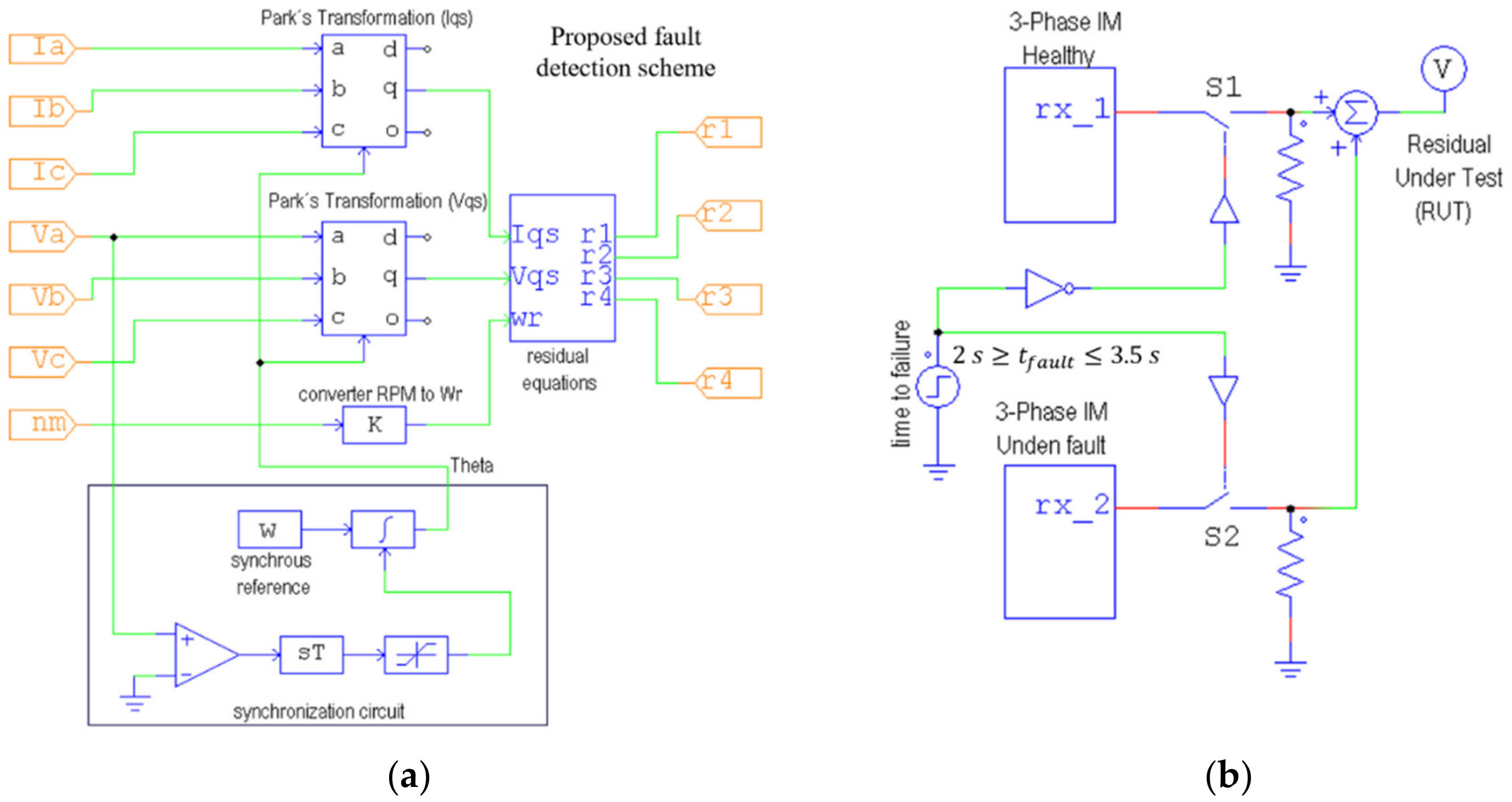
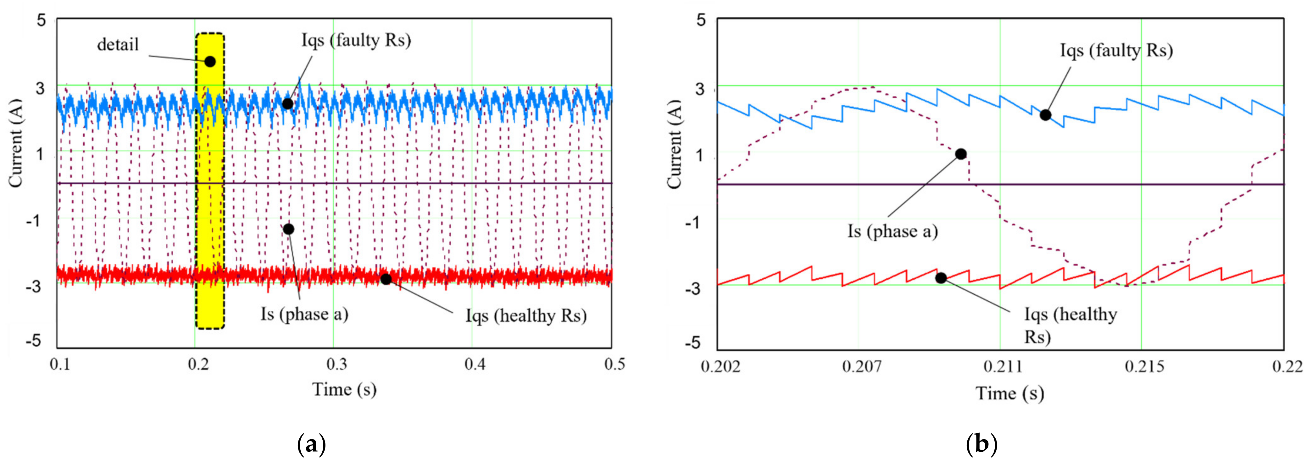
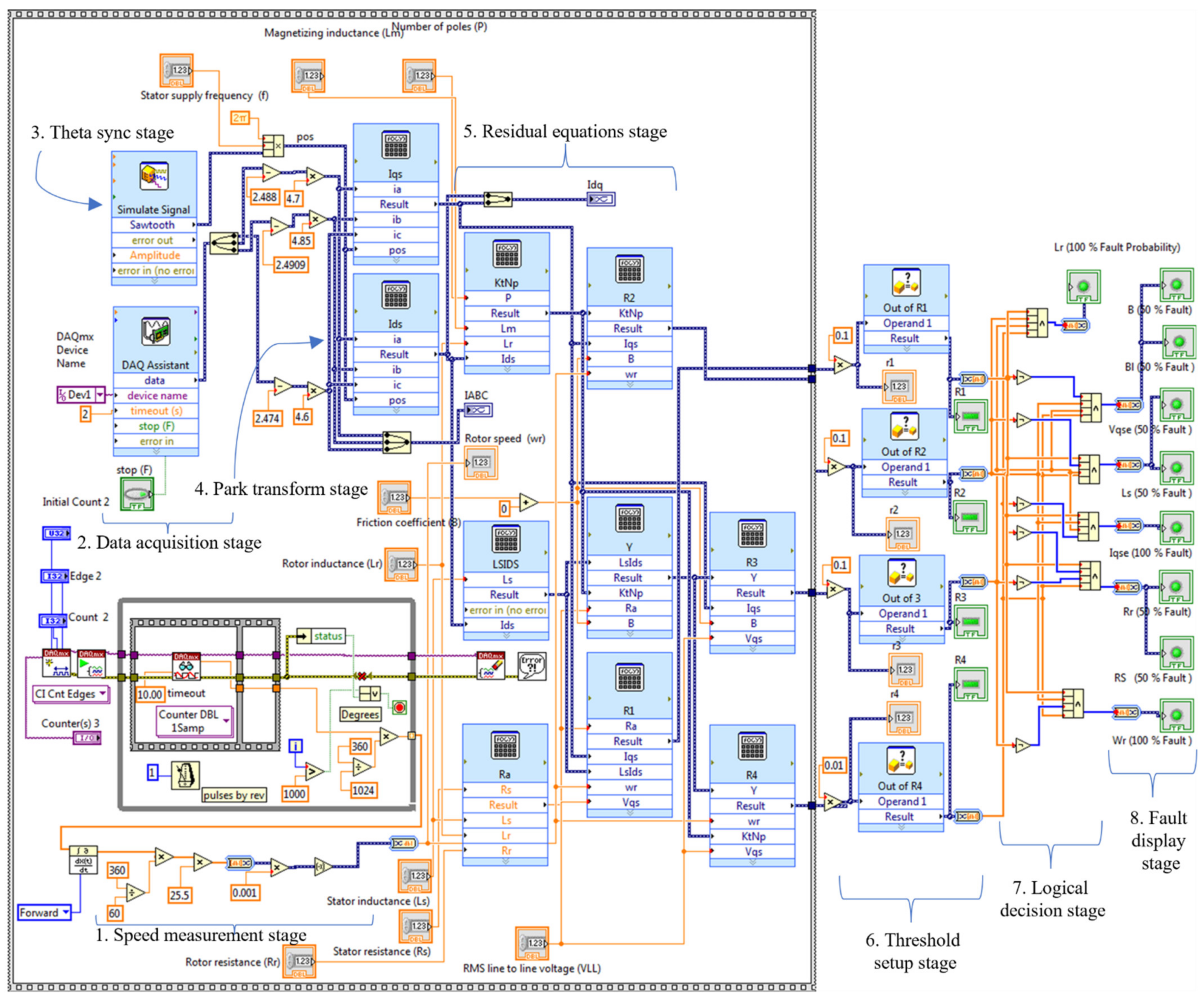
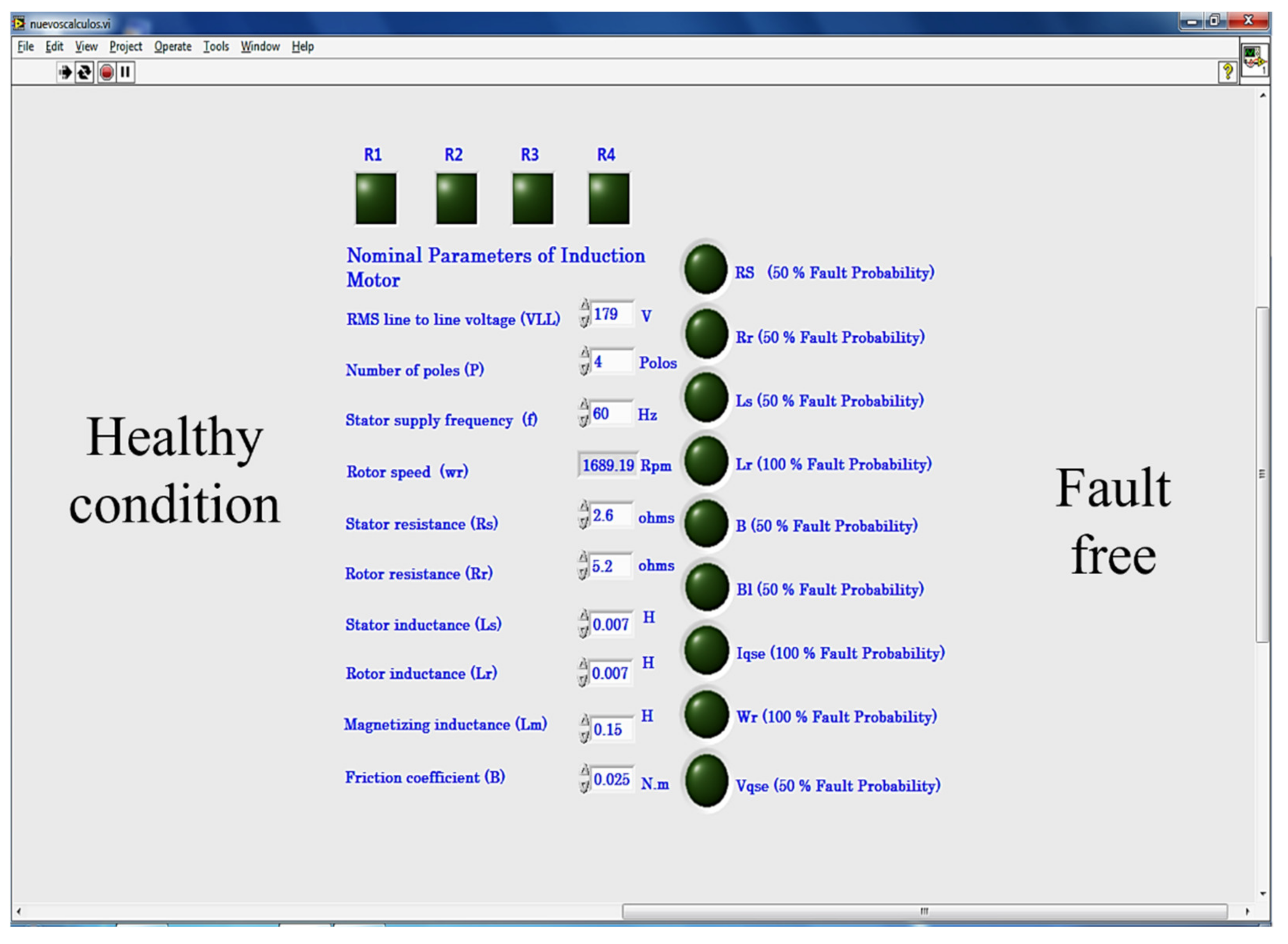
4.1. Simulation Setup

An alternative, in addition to experimental tests, to validate the fault detection system on the 3PIM working in the synchronous reference frame is to use a reliable simulation software with a wide availability of models in power electronics, electric machine drives, and dynamic systems, such as the power electronic circuit simulation (PSIM) software package, developed by PowerSim company. Figure 3 shows the main simulation and experimental scheme for fault diagnosis in the 3PIM using PSIM, and the detail of the proposed fault detection scheme is shown in Figure 4.

The instrumentation system is highlighted in the main simulation and experimental scheme composed of: 3-phase source, current, voltage and speed sensors, mechanical load, proposed fault detection sub-scheme, 3-phase induction motor under test, as well as the residual measurement points (r1, r2, r3, and r4). Figure 4a shows the detail of the sub-scheme of the main simulation where the measurement of $I_{qs}$ and $V_{qs}$ using Park’s transformation, the theta synchronization circuit, the speed converter, and the residual equations set are carried out. On the other hand, Figure 4b shows the general test configuration of the fault detection system used to simulate the residual behavior with a healthy environment (3-Phase IM Healthy) plus the under-fault environment (3-Phase IM Under Fault). In this figure, it can be seen that the under-fault time is activated by a pair of complementary switches S1 and S2, which are controlled by an impulse source with a fault time $2 \mathrm{s} \ge t_{fault}\le 3.5 \mathrm{s}$. Therefore, the result of the residual under test (RUT) hides the dynamic behavior of the healthy and under-fault residue because the 3PIM modules are operating from t = 0. In this way, only the turn-on transient of the fault-free module could be appreciated, but the data acquisition starts when t > 0.5 s with a sampling time of 20 ms. Then, the smoothed and steady-state behavior during the fault-free and under-fault conditions is considered.

Figure 5 and Figure 6 show the behavior of the RUT in healthy and under-fault condition for seven different failure scenarios ($R_s$, $R_r$, $L_s$, $L_r$, $I_{qs}$, $V_{qs}$, ${\omega }_r$) with parametric values up and down at 50% of their nominal value, respectively. Likewise, the residual variation affected in each failure scenario is highlighted and is consistent with the simplified equation behavior (37). Table 1 shows the simplified behavior of all residuals related to each under-fault parameter, where the term “I” represents a positive or negative parametric change that depends on the increasing or decreasing fault trend, as shown in Figure 4 and Figure 5, respectively. Likewise, in Table 1, an identical residual behavior or signature can be observed for two different fault conditions, as in the case of R_s-R_r, B-B_l, and L_s-V_qs. This reduces the probability of detection to 50% with respect to the affected parameter. However, the proposed fault detection scheme could be complemented with another detection scheme based on an electrical and/or mechanical model to distinguish the fault in a particular way. Another problem found in this proposed scheme is that in the abc/d-q transformation the possibility of detecting the affected phase or sensor is lost, and only generalized faults are obtained. Although the identification of the damaged phase or sensor can be obtained by interpreting the current and voltage phase unbalance, as mentioned in [40,41].

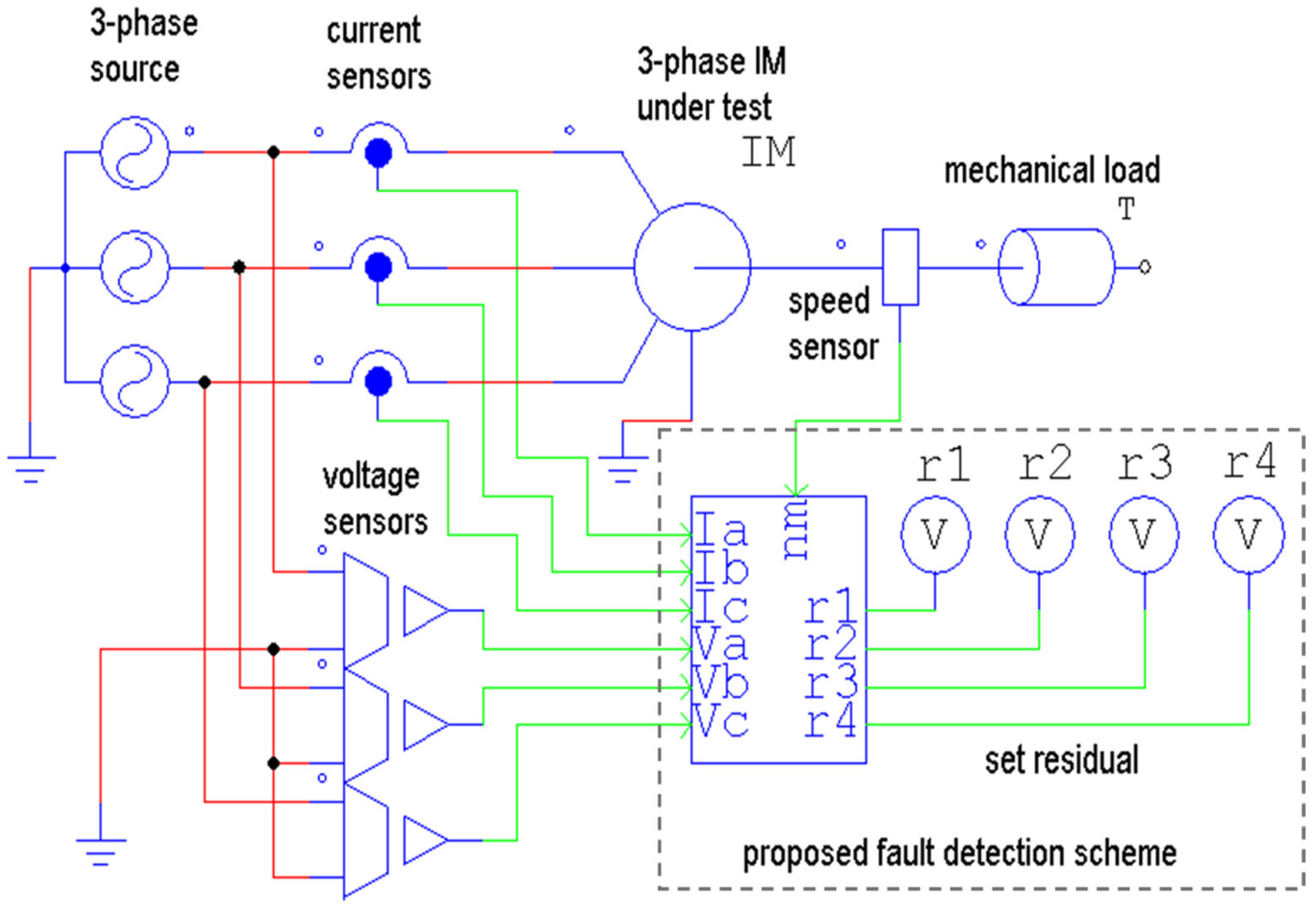
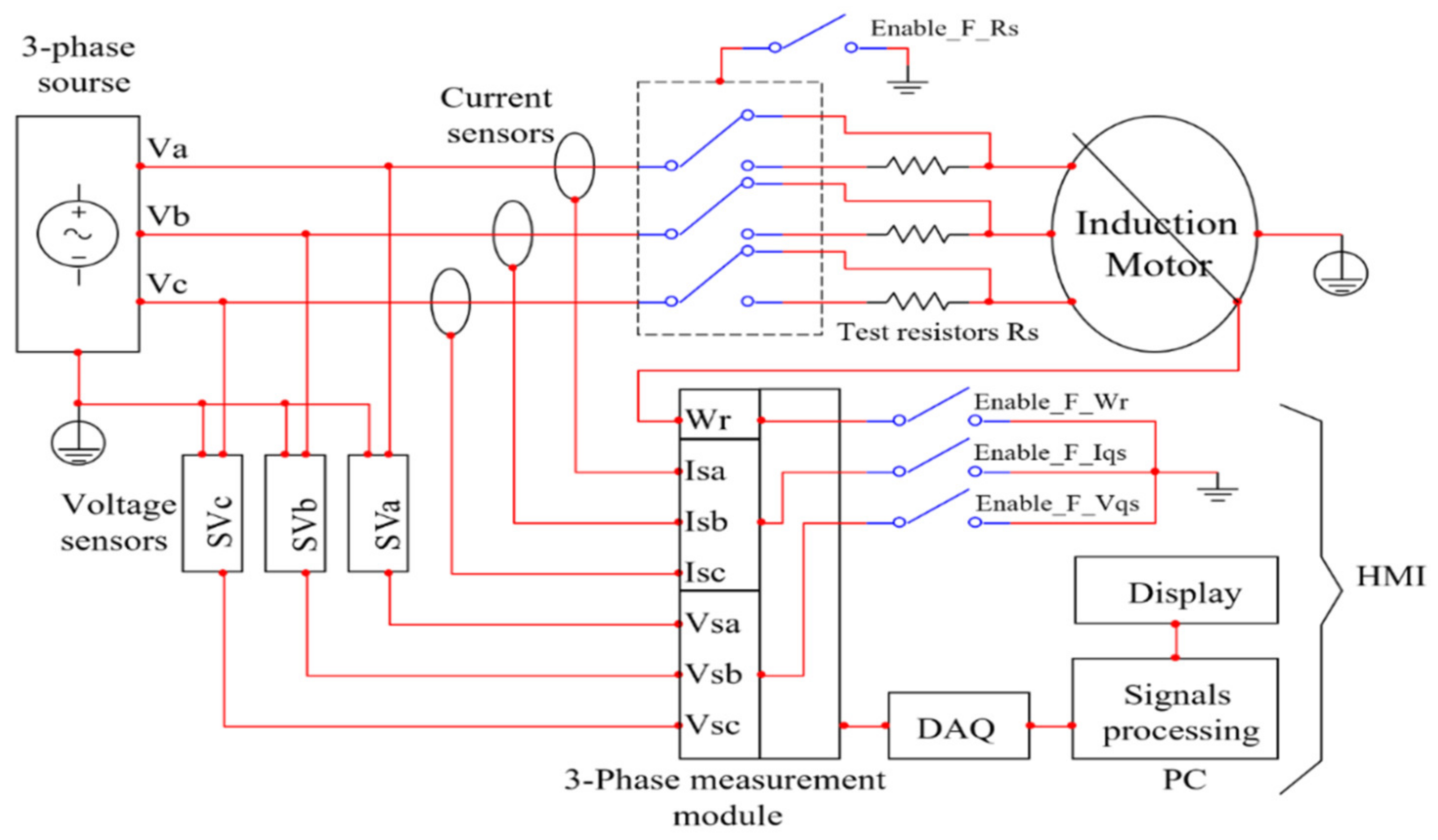
4.2. Experimental Setup

To validate the approach proposed in Section 3 through experimental tests, it is necessary to be able to change the motor parameters physically. This is very complicated because that is only accessible by abrupt faults through destructive tests. Regarding the stator side, a non-abrupt fault emulation in the inductance may be accessible in the stator winding, but the stator resistance will be altered. On the other hand, an emulation of an abrupt and increasing fault in stator resistance by adding series resistances to the stator windings will not affect the stator inductance. The proposal in this experimental section is to implement the proposed fault detection scheme in a human machine interface (HMI) and emulate fault scenarios for current, voltage, and speed sensors, as well as build a stator resistance fault scenario by adding resistors in series to the winding of each phase of the 3PIM, which does not affect the stator inductance.

Figure 7 shows a block diagram of the proposed scheme to diagnose faults in the sensors and stator resistance. In general, the 3PIM is powered by a balanced 3-phase source, and through an HMI, the fault diagnosis is carried out. In particular, the currents, voltages, and speed measurements are carried out through a 3-phase measurement module, which is enabled by three digital signals, the data are entered into a personal computer (PC) through a data acquisition (DAQ) board and subsequently processed with the LabVIEW software, and finally, on a PC screen, the results obtained are displayed. Taking into account a practical point of view, one way to carry out the experimental tests and avoid destructive tests is only to emulate noninvasive failures in the sensors and parameter of the proposed scheme, as shown in Figure 7. In that way, to emulate sensor faults, the output signal of current-I_qs, voltage-V_qs, and speed-ω_r sensors are disabled through digital signals Enable_F_Iqs, Enable_F_Vqs, and Enable_F_Wr, respectively. Regarding 3PIM parameter faults, a simple noninvasive and nondestructive test is adding a set of resistors in series with the stator winding to emulate fault in R_s (increasing fault) through the digital signal Enable_F_Rs. Then, the full detection algorithm is executed. On the other hand, when $R_s$ increases, many 3PIM parameters are modified, prevailing the negative value for $I_{qs}$ and the positive value for $R_a$, consistent with the residuals r1 and r4 in (37) and displayed in Figure 5. Now, a practical way to validate the proper behavior of the HMI for the fault-free and under-fault conditions is using an oscilloscope with data storage capacity for measurement the phase stator current and using a mathematical software as MATHCAD for to process and graph the D-Q currents. An example of the proper performance of the proposed scheme with respect to stator resistance failure is shown in Figure 8. In this figure, it can be seen that phase currents ($I_{sa}$, $I_{sb}$) and the turn-on transient time (0–0.1 s) are omitted for better visibility, and it is observed that the absolute increasing trend of the healthy and faulty current-I_qs are consistent with (37). Figure 8b highlights a detail of this behavior and shows signals with oscillatory behavior attributed to the oscilloscope sampling rate for stator current data acquisition (range 0 to 0.5 s with 512 samples per second).

Figure 9 shows the photograph of the experimental setup to diagnose failures in 3PIM, taking into account the block diagram of the proposed scheme in Figure 7. The 3PIM parameters were previously characterized by electrical measurements, and the instrumental equipment used is shown in

Table 2. Instrumental equipment specifications.

Description	Value
3-phase power supply	Manufacturer Delorenzo (Rozzano, Milan, Italy), model DL1013M3
3-phase induction motor	Manufacturer Delorenzo (Rozzano, Milan, Italy), model DL10115A1, 300 W, star configuration and access to neutral terminal
3-phase measurement module	Manufacturer K-oz Soluciones integrales (Merida, Yucatan Mexico), model MOD.MEW-3P-180V15A-MIX
Encoder speed sensor	Manufacturer Yumo Electric Co. (Yueqing city, China), model E6B2-CWZ3E, resolution 1024 pulses/rev
DAQ board	Manufacturer National Instruments (Austin, TX, USA), model PCI-SCB-100
PC Intel Pentium	Manufacture Lanix (Hermosillo, Mexico), model Titan.
PC Screen	Manufacturer Lanix (Hermosillo, Mexico), model 900W, screen 24 inch
Test resistors	Manufacturer Delorenzo (Rozzano, Milan, Italy), model DL2643, 3-phase 1 Ω

.

Figure 10 shows the fault detection algorithm implemented in the graphical programming environment of the LabVIEW software. In this figure, all the stages of development can be seen, as follows: 1. Encoder pulse measurement to interpret angular velocity, 2. DAQ wizard tool to calibrate the measurement sensors, 3. Phase “a” voltage-zero-crossing detector to generate synchronous position of Theta, 4. Dedicated math tool for Park transformation, 5. Algebraic equation editing tool to implement residual equations, 6. Electrical magnitude comparator tool to configure detection thresholds, 7. Logical evaluation to implement the residual matrix, and 8. Logic deployment to interpret the outputs on the HMI. A detail of the HMI screen in the fault-free condition is shown in Figure 11. The input data in the interface are the nominal parameters of the 3PIM under test, and the output data are the light-emitting diode (LED) type lamps corresponding to the affected residues and the probability of failure. Figure 12 shows the HMI residual screen for the under-fault cases in $I_{qs}$, $V_{qs}$, ${\omega }_r$_, and $R_s$, respectively.

5. Discussion

The definition and use of the terms $R_a$, $K_a$, $T_a$, $K_f$ allows matching Equations (28) and (29) with the DC motor model proposed in [39]. The considerations taken into account in this work limit the isolation of faults in steady-state operation because in (36), the derivative terms of the input signals are neglected. The advantage is that the residual set obtained turns out to be a very simplified algebraic term with respect to the expression obtained in [22], so a very modest electronic development with LED lights as a qualitative diagnostic element can be carried out at a reduced cost. Another advantage, with respect to other diagnostic techniques mentioned in the introduction section, is that the proposed scheme allows detecting a large set of damaged parameters without the need to use different techniques for each parameter.

The qualitative results obtained in the simulation and experimental test during the steady state operation of 3PIM show a consistent behavior, which validates the proposed scheme by contrasting the theoretical part (Table 1) with the experimental part (Figure 12). It is to be expected that in the experimental test, there are quantitative inconsistencies due to the linearization and the practical considerations taken into account in the 3PIM model, so the tuning of thresholds both in the simulation and in the experiment was carried out heuristically. On the other hand, when the friction coefficients are no longer negligible in r3 and r4, according to (37), then the diagnostic matrix is no longer valid. In this sense, load disturbances can cause false alarms during the transient part, and faults will be constant in stable state when the load exceeds the tuned thresholds.

We have to say that the main disadvantage is that the detection system is based on a mathematical transformation, Park’s transform, which considers an ideally balanced 3-phase system, which is practically impossible to obtain, so the current and voltage signals in synchronous regimen must be compensated beforehand. Likewise, the current sensors, voltage sensors, and parameter faults of each phase must be symmetrical. A possible improvement in the future is to consider the operating temperature, which affects some electrical parameters of the IM, so a robust design in parity equations could improve the residual performance.

References

1. Report of Large Motor Reliability Survey of Industrial and Commercial Installations, Part II. IEEE Trans. Ind. Applicat. 1985, IA-21, 865–872. [CrossRef]
2. Delgado-Arredondo, P.A.; Morinigo-Sotelo, D.; Osornio-Rios, R.A.; Avina-Cervantes, J.G.; Rostro-Gonzalez, H.; Romero-Troncoso, R.d.J. Methodology for Fault Detection in Induction Motors via Sound and Vibration Signals. Mech. Syst. Signal Process. 2017, 83, 568–589. [Google Scholar] [CrossRef]
3. Mazzoletti, M.A.; Donolo, P.D.; Pezzani, C.M.; Oliveira, M.O.; Bossio, G.R.; De Angelo, C.H. Stator Faults Detection on Induction Motors Using Harmonic Sequence Current Components Analysis. IEEE Lat. Am. Trans. 2021, 19, 726–734. [Google Scholar] [CrossRef]
4. Choudhary, A.; Goyal, D.; Shimi, S.L.; Akula, A. Condition Monitoring and Fault Diagnosis of Induction Motors: A Review. Arch. Computat. Methods Eng. 2019, 26, 1221–1238. [Google Scholar] [CrossRef]
5. Goh, Y.-J.; Kim, K.-M. Inter-Turn Short Circuit Diagnosis Using New D-Q Synchronous Min–Max Coordinate System and Linear Discriminant Analysis. Appl. Sci. 2020, 10, 1996. [Google Scholar] [CrossRef] [Green Version]
6. Goh, Y.-J.; Kim, O. Linear Method for Diagnosis of Inter-Turn Short Circuits in 3-Phase Induction Motors. Appl. Sci. 2019, 9, 4822. [Google Scholar] [CrossRef] [Green Version]
7. Kallesoe, C.S.; Izadi-Zamanabadi, R.; Vadstrup, P.; Rasmussen, H. Observer-Based Estimation of Stator-Winding Faults in Delta-Connected Induction Motors: A Linear Matrix Inequality Approach. IEEE Trans. Ind. Appl. 2007, 43, 1022–1031. [Google Scholar] [CrossRef]
8. Hegde, V.; Sathyanarayana Rao, M.G. Detection of Stator Winding Inter-Turn Short Circuit Fault in Induction Motor Using Vibration Signals by MEMS Accelerometer. Electr. Power Compon. Syst. 2017, 45, 1463–1473. [Google Scholar] [CrossRef]
9. Mejia-Barron, A.; Tapia-Tinoco, G.; Razo-Hernandez, J.R.; Valtierra-Rodriguez, M.; Granados-Lieberman, D. A Neural Network-Based Model for MCSA of Inter-Turn Short-Circuit Faults in Induction Motors and Its Power Hardware in the Loop Simulation. Comput. Electr. Eng. 2021, 93, 107234. [Google Scholar] [CrossRef]
10. Skowron, M.; Orlowska-Kowalska, T.; Wolkiewicz, M.; Kowalski, C.T. Convolutional Neural Network-Based Stator Current Data-Driven Incipient Stator Fault Diagnosis of Inverter-Fed Induction Motor. Energies 2020, 13, 1475. [Google Scholar] [CrossRef]
11. Hassan, O.E.; Amer, M.; Abdelsalam, A.K.; Williams, B.W. Induction Motor Broken Rotor Bar Fault Detection Techniques Based on Fault Signature Analysis—A Review. IET Electr. Power Appl. 2018, 12, 895–907. [Google Scholar] [CrossRef]
12. Asad, B.; Vaimann, T.; Rassõlkin, A.; Kallaste, A.; Belahcen, A. A Survey of Broken Rotor Bar Fault Diagnostic Methods of Induction Motor. Electr. Control Commun. Eng. 2018, 14, 117–124. [Google Scholar] [CrossRef] [Green Version]
13. Duda, A.; Drozdowski, P. Induction Motor Fault Diagnosis Based on Zero-Sequence Current Analysis. Energies 2020, 13, 6528. [Google Scholar] [CrossRef]
14. Esam El-Dine Atta, M.; Ibrahim, D.K.; Gilany, M.I. Broken Bar Faults Detection Under Induction Motor Starting Conditions Using the Optimized Stockwell Transform and Adaptive Time–Frequency Filter. IEEE Trans. Instrum. Meas. 2021, 70, 3518110. [Google Scholar] [CrossRef]
15. Defdaf, M.; Berrabah, F.; Chebabhi, A.; Cherif, B.D.E. A New Transform Discrete Wavelet Technique Based on Artificial Neural Network for Induction Motor Broken Rotor Bar Faults Diagnosis. Int. Trans. Electr. Energ. Syst 2021, 31, e12807. [Google Scholar] [CrossRef]
16. Alshorman, O.; Alshorman, A. A Review of Intelligent Methods for Condition Monitoring and Fault Diagnosis of Stator and Rotor Faults of Induction Machines. IJECE 2021, 11, 2820. [Google Scholar] [CrossRef]
17. Wang, D.; Liang, Y.; Li, C.; Yang, P.; Zhou, C.; Gao, L. Thermal Equivalent Network Method for Calculating Stator Temperature of a Shielding Induction Motor. Int. J. Therm. Sci. 2020, 147, 106149. [Google Scholar] [CrossRef]
18. Areias, I.A.d.S.; Borges da Silva, L.E.; Bonaldi, E.L.; de Lacerda de Oliveira, L.E.; Lambert-Torres, G.; Bernardes, V.A. Evaluation of Current Signature in Bearing Defects by Envelope Analysis of the Vibration in Induction Motors. Energies 2019, 12, 4029. [Google Scholar] [CrossRef] [Green Version]
19. Yuejun, A.; Zhiheng, Z.; Ming, L.; Guangyu, W.; Xiangling, K.; Zaihang, L. Influence of Asymmetrical Stator Axes on the Electromagnetic Field and Driving Characteristics of Canned Induction Motor. IET Electr. Power Appl. 2019, 13, 1229–1239. [Google Scholar] [CrossRef]
20. Gertler, J.J. Fault Detection and Diagnosis in Engineering Systems, 1st ed.; CRC Press: Boca Raton, FL, USA, 2017; ISBN 978-0-203-75612-6. [Google Scholar]
21. Chan, C.W.; Hua, S.; Hong-Yue, Z. Application of Fully Decoupled Parity Equation in Fault Detection and Identification of DC Motors. IEEE Trans. Ind. Electron. 2006, 53, 1277–1284. [Google Scholar] [CrossRef]
22. Bouattour, J. Diagnosing Parametric Faults in Induction Motors with Nonlinear Parity Relations. IFAC Proc. Vol. 2000, 33, 971–976. [Google Scholar] [CrossRef]
23. Isermann, R. Supervision, Fault-Detection and Fault-Diagnosis Methods—An Introduction. Control Eng. Pract. 1997, 5, 639–652. [Google Scholar] [CrossRef]
24. Chang, H.-C.; Jheng, Y.-M.; Kuo, C.-C.; Hsueh, Y.-M. Induction Motors Condition Monitoring System with Fault Diagnosis Using a Hybrid Approach. Energies 2019, 12, 1471. [Google Scholar] [CrossRef] [Green Version]
25. Khojet El Khil, S.; Jlassi, I.; Estima, J.O.; Mrabet-Bellaaj, N.; Marques Cardoso, A.J. Current Sensor Fault Detection and Isolation Method for PMSM Drives, Using Average Normalised Currents. Electron. Lett. 2016, 52, 1434–1436. [Google Scholar] [CrossRef]
26. Wang, Z.; Chang, C.S. Online Fault Detection of Induction Motors Using Frequency Domain Independent Components Analysis. In Proceedings of the 2011 IEEE International Symposium on Industrial Electronics, Gdansk, Poland, 27–30 June 2011; pp. 2132–2137. [Google Scholar] [CrossRef]
27. Chua, T.W.; Tan, W.W.; Wang, Z.-X.; Chang, C.S. Hybrid Time-Frequency Domain Analysis for Inverter-Fed Induction Motor Fault Detection. In Proceedings of the 2010 IEEE International Symposium on Industrial Electronics, Bari, Italy, 4–7 July 2010; pp. 1633–1638. [Google Scholar] [CrossRef]
28. Yang, T.; Pen, H.; Wang, Z.; Chang, C.S. Feature Knowledge Based Fault Detection of Induction Motors Through the Analysis of Stator Current Data. IEEE Trans. Instrum. Meas. 2016, 65, 549–558. [Google Scholar] [CrossRef]
29. Moseler, O.; Isermann, R. Application of Model-Based Fault Detection to a Brushless DC Motor. IEEE Trans. Ind. Electron. 2000, 47, 1015–1020. [Google Scholar] [CrossRef]
30. Che Mid, E.; Dua, V. Model-Based Parameter Estimation for Fault Detection Using Multiparametric Programming. Ind. Eng. Chem. Res. 2017, 56, 8000–8015. [Google Scholar] [CrossRef]
31. Decker, S.; Stoss, J.; Liske, A.; Brodatzki, M.; Kolb, J.; Braun, M. Online Parameter Identification of Permanent Magnet Synchronous Machines with Nonlinear Magnetics Based on the Inverter Induced Current Slopes and the Dq-System Equations. In Proceedings of the 2019 21st European Conference on Power Electronics and Applications (EPE ’19 ECCE Europe), Genova, Italy, 3–5 September 2019; pp. 1–10. [Google Scholar] [CrossRef]
32. Rodriguez, M.A.; Hernandez, M.; Mendez, F.; Sibaja, P.; Hernandez, L. A Simple Fault Detection of Induction Motor by Using Parity Equations. In Proceedings of the 8th IEEE Symposium on Diagnostics for Electrical Machines, Power Electronics & Drives, Bologna, Italy, 5–8 September 2011; pp. 573–579. [Google Scholar] [CrossRef]
33. Chulines, E.; Rodríguez, M.A.; Duran, I.; Sánchez, R. Simplified Model of a Three-Phase Induction Motor for Fault Diagnostic Using the Synchronous Reference Frame DQ and Parity Equations. IFAC-Pap. 2018, 51, 662–667. [Google Scholar] [CrossRef]
34. Isermann, R. Fault-Diagnosis Systems; Springer: Berlin/Heidelberg, Germany, 2006; ISBN 978-3-540-24112-6. [Google Scholar] [CrossRef]
35. Gertler, J.; Singer, D. A New Structural Framework for Parity Equation-Based Failure Detection and Isolation. Automatica 1990, 26, 381–388. [Google Scholar] [CrossRef]
36. Nandi, S.; Toliyat, H.A.; Li, X. Condition Monitoring and Fault Diagnosis of Electrical Motors—A Review. IEEE Trans. Energy Convers. 2005, 20, 719–729. [Google Scholar] [CrossRef]
37. Krause, P.; Wasynczuk, O.; Sudhoff, S.; Pekarek, S. (Eds.) Analysis of Electric Machinery and Drive Systems; John Wiley & Sons, Inc.: Hoboken, NJ, USA, 2013; ISBN 978-1-118-52433-6. [Google Scholar]
38. Kazmierkowski, M.P. Electric Motor Drives: Modeling, Analysis and Control, R. Krishan, Prentice-Hall, Upper Saddle River, NJ, 2001, Xxviii + 626 Pp. ISBN 0-13-0910147: BOOK REVIEW. Int. J. Robust Nonlinear Control 2004, 14, 767–769. [Google Scholar] [CrossRef]
39. Höfling, T.; Isermann, R. Fault Detection Based on Adaptive Parity Equations and Single-Parameter Tracking. Control Eng. Pract. 1996, 4, 1361–1369. [Google Scholar] [CrossRef]
40. Rodriguez-Blanco, M.A.; Golikov, V.; Vazquez-Avila, J.L.; Samovarov, O.; Sanchez-Lara, R.; Osorio-Sánchez, R.; Pérez-Ramírez, A. Comprehensive and Simplified Fault Diagnosis for Three-Phase Induction Motor Using Parity Equation Approach in Stator Current Reference Frame. Machines 2022, 10, 379. [Google Scholar] [CrossRef]
41. Bakhri, S.; Ertugrul, N. A Negative Sequence Current Phasor Compensation Technique for the Accurate Detection of Stator Shorted Turn Faults in Induction Motors. Energies 2022, 15, 3100. [Google Scholar] [CrossRef]
Figure 1. Simple parity equation scheme in state-space model.
Energies 15 08372 g001
Figure 2. Block diagram of the 3PIM model matched with the DC motor model.
Energies 15 08372 g002
Figure 3. Main simulation and experimental scheme for fault diagnosis in the 3PIM.
Energies 15 08372 g003
Figure 4. Detail of proposed fault detection scheme: (a) Proposed fault detection scheme; (b) residual under test with healthy and faulty 3PIM.
Energies 15 08372 g004
Figure 5. Residual behavior with up parametric variation to +50% of nominal value.
Energies 15 08372 g005
Figure 6. Residual behavior with down parametric variation to −50% of nominal value.
Energies 15 08372 g006
Figure 7. Block diagram of proposed experimental scheme for 3PIM fault detection.
Energies 15 08372 g007
Figure 8. Measurement of current I q s in fault-free and under-fault condition: (a) I q s with healthy and faulty R s , (b) details of I q s .
Energies 15 08372 g008
Figure 9. Photograph of experimental setup.
Energies 15 08372 g009
Figure 10. Fault detection algorithm implemented in LabVIEW.
Energies 15 08372 g010
Figure 11. Screen of HMI for the 3PIM fault detection in the fault-free case.
Energies 15 08372 g011
Figure 12. HMI for different residual conditions under fault.
Energies 15 08372 g012