Abstract
This paper presents a novel observer-based robust fault predictive control (OBRFPC) approach for a wind turbine time-delay system subject to constraints, actuator/sensor faults, and external disturbances. The proposed approach is based on an augmented state-space representation that contains state-space variables and estimation errors. The proposed augmented representation is then used to synthesize a robust predictive controller. In addition, an observer is developed and used to estimate both state variables and actuator/sensor faults. To ensure that the proposed approach has disturbance rejection capabilities, the disturbance estimates were merged with the prediction model. In addition, the disturbance rejection capabilities and fault tolerance were insured by formulating the control process as an optimization problem subject to constraints in terms of linear matrix inequalities (LMIs). As a result, the controller gains are acquired by solving an LMI problem to guarantee input-to-state stability in the presence of sensor and actuator faults. A simulation example is conducted on a nonlinear wind turbine (1 MW) model with 3 blades, a horizontal axis, and upwind variable speed subject to actuator/sensor faults in the pitch system. The results demonstrate the ability of the proposed method in dealing with nonlinear systems subject to external disturbances and keeping the control performance acceptable in the presence of actuator/sensor faults.
1. Introduction
Wind energy research and technology has been experiencing a strong revival of interest since the early 1990s, particularly in the European Union, where its annual growth is around 20%. However, due to the complexity of the wind turbine structure and challenging operational conditions, several types of actuator or/and sensor faults are frequently encountered, which may drive the system far from its main objectives and even cause significant damage to the system’s components in certain critical cases. When faults appear in sensors and/or actuators, the characteristics of the sensors and/or actuators can change over time, and this will affect the performance of the designed controller and even the stability of the overall system [1,2,3]. As a consequence, the implementation of fault tolerant control (FTC) systems is crucial in order to ensure acceptable performance and to maintain certain properties of the system such as stability and performance [4,5].
Generally, consideration of actuator faults that may happen on the steering system of the blades is important to ensure acceptable performance of the control system. Many researchers have proposed several FTC algorithms to deal with actuator faults where the basic approach is done by compensating the constant (zero) control of the actuator faulty actuator by distributing the control (or the effort) over the non-defective actuators [6,7]. Based on the backpropagation artificial neural network (BPANN), an estimator is developed and employed to estimate the pitch rotor and generator speeds to detect the faults in these actuators with unknown inputs, such as modeling defects, perturbations, disturbances, and parameters uncertainties [8,9]. An active fault-tolerant control method is proposed in [10] to overcome the partial loss of actuator effectiveness. Data-driven fault detection and diagnosis algorithm is presented in [11] where historical data of the turbine is used instead of the model for the estimation process. An approach based on unknown input observers for detection and isolation of sensor faults on the rotor speed and generator speed is also proposed, in which the speed estimation results obtained by the observer are used in the current control process [12]. A nonlinear static state feedback control with asymptotic tracking at the optimal rotation speed is developed in [13] to compensate for sensor faults in the maximum power capturing procedure of the wind turbine. A fault tolerant control scheme using the virtual actuators and sensors is proposed in [14] to deal with both sensor and actuator faults. In [15], the analytical redundancy of the system is used to harvest fault information. Moreover, the FTTC strategy, proposed in [16], is designed to maintain the wind turbine nominal controller without any change in the fault and non-fault cases.
Recently, fault tolerance techniques for the robust model predictive control design problem have gained more attraction in dealing with faulty nonlinear systems [17,18,19,20]. In [21], a new robust constrained model predictive fault-tolerant control method was proposed for uncertain time-delay systems with unknown disturbances and partial actuator failures. In this approach, a control law with an optimized cost and H∞ performance was derived where feasible solutions were obtained by solving the LMI constraints. In [22], an approach was proposed for evaluating the actuator fault tolerance of a nonlinear model predictive control (NMPC) model. The proposed approach used the zonotopes method to evaluate viability sets, while a new algorithm is developed and implemented to assess the tolerance of the NMPC controller. In [23], an MPC scheme based on a min-max optimization algorithm was proposed to assure the satisfaction of constraints of the control subject to pitch actuator fault. Furthermore, actuators or/and sensor faults in the pitch system have been considered in many research papers [17,24,25] where the FTC schemes are designed to compensate for the effects of faults. In addition, a novel fault tolerant scheme with a system health management module and MPC was built up by using a fatigue-based model and rain-flow counting in [26]. In [27], a fault-tolerant MPC based on a min-max approach was developed and designed to guarantee the constraint satisfaction of the system with the pitch actuator fault.
Resultantly, the consideration of faults of sensors and/or actuators in the control schemes is important to assure acceptable performance when faults occur where the objective is to maintain certain properties, such as stability, of the system. However, most of the research that has been conducted on FTC approaches deals with either sensor or actuator faults for the MPC controller. Only limited investigations can handle both sensor and actuator faults simultaneously. In [28,29], the authors have proposed a predictive control with multiplicative sensor and actuator faults, which does not present modeling close to the defects. It should be noted that the states of many control systems are not always measurable, especially in the presence of additive faults. In [29], a predictive fault tolerant control scheme is developed to capture the maximum power for wind turbines in the partial-load region, and based on the sliding mode control, an observer is designed to estimate the actual states and actuator/sensor faults simultaneously in a class of uncertain systems. Unfortunately, only a few research papers have considered robust constrained model predictive fault-tolerant control for time-delay systems that also copes with both input and output constraints, sensor and actuator faults, and external disturbances.
In this paper, an observer-based robust model predictive control design is proposed and investigated to stabilize a wind turbine-constrained time-delays system with sensor and actuator faults and subject to external disturbances. Firstly, an augmented closed-loop system with the state and sensor/actuator faults observation error is proposed for describing the system. The stability conditions of closed-loop systems are designed to consider the presence of input constraints, time delay, and additive sensor and/or actuator faults. The main objective of this research is to synthesize the proposed OBRFPC approach that deals with time-delays systems in the presence of sensor and actuator faults and subject to external disturbances. In order to achieve the above goals, an LMI-based minimization problem is formulated to solve the robust control design. To ensure robust stability and performance, such a robust control strategy can be realized by employing several mathematical lemmas and well-known linear matrix inequalities theorems. In addition, the robustness of the system performance is analytically shown in the worst-case conditions. The observer-based RMPC scheme can reduce the effect of faults and disturbances and guarantee the stability of the wind turbine system even in the presence of the actuator faults, sensor faults, and wind speed external disturbances.
This paper is organized as follows: Section 2 provides the problem formulation. Section 3 describes the design of observers to estimate the states of the system and sensor and actuator faults. In Section 4, we present an observer-based controller MPC to stabilize the system with time delays using the Lyapupnov–Krasovskii functions. Section 5 demonstrates a case study in which the proposed method is applied and investigated. Finally, certain remarks and conclusions are provided in Section 6.
Notation 1.
The symbols used in this paper are standard unless otherwise specified.is the controller gains matrices andis the observer gain matrix.is a varying delay.denotes the-dimensional Euclidean space, andare the set of,,real matrices, respectively.andrepresent the zero and the identity matrices with proper dimensions, respectively.,,,,,, andare the symmetric positive definite matrices. Matrix() signifies that each entry ofis non-negative (positive).are the weighting matrices.
2. Problem Statement
In this section, two cases are studied: a system with both sensor and actuator faults in the absence of external disturbance and time-delay systems with the external disturbance . Firstly, an observer for estimating the states of the system (1) and the corresponding faults is designed. Secondly, an observer-based RMPC is established based on the designed observer.
- Case 1. Sensor/Actuator Faults
Consider the following discrete-time systems:
The control action is required to satisfy the following constraints.
where is the upper constraint of the control input.
In this paper, we consider both types (sensor and actuator) of faults. When a sensor fault occurs, the real measurement of the system output can be described by:
where is the vector of additive sensor faults.
In addition, when an actuator fault occurs, the control input torque can be represented by
where the is the actuator’s fault, and the is the control input signal.
In the following, the model of the wind turbine (1) is augmented by a state that represents the effective wind speed disturbances . In addition, we design a wind estimator to estimate the fictitious wind speed, which is an unmeasurable quantity.
In this work, the following Lemmas and assumptions are used.
Lemma 1.
(Schur Complement). [30] Given any real matrices,, andwithand, we have
If and only if
The following assumptions and definitions are needed to acquire our main results.
Assumption 1.
Defining the following variables
The following augmented matrices and variables are defined:
The augmented system can be obtained as:
Remark 1.
It is worth noting that the state vectorin (5) is a combination of the states, the actuator faultand the sensor fault. Therefore, if the fault-tolerant observer is designed for the augmented system in (5), the estimation of the states and faults can be obtained simultaneously.
To estimate the state of the system in Equation (1), , actuator fault , and sensor fault , an augmented observer is designed for the discrete-time system in (5):
where are the observer state and estimated state, respectively. The matrix is the gain of the observer.
In addition, an observer-based state-feedback controller is considered such as:
The main objective is then to propose an observer-based feedback fault-tolerant controller that can assure that the system in Equation (1), subject to both the sensor and actuator faults, is asymptotically stable with OBRFPC performance.
3. Observer-Based Model Predictive Control
In this section, an observer-based model predictive controller is designed for the linear discrete-time systems in Equation (1) subject to sensor/actuator faults. First, the following state observer is adopted to estimate the augmented state vector of the system:
where is the estimation of . The matrix is the gain of the state observer. We consider an observer-based state-feedback control strategy as:
Define the state estimation .
From Equations (5) and (8), the estimation error can be expressed as:
Substituting (7) into (5), we have
For simplicity, denote ,
Now, we consider the problem of minimizing the following worst-case quadratic objective function with an infinite horizon:
such as .
The weighting matrices and are known positive-definite matrices.
The following theorem is used to present the stability condition for the overall closed-loop system given in Equation (11):
Theorem 1.
Given the augmented state-space model in (5), the state-feedback controller given by Equation (7) robustly stabilizes the discrete-time system, in Equation (5), subject to actuator faults, disturbances, and time delays. There are symmetric positive definite matrices,,,,, andand a positive scalarsatisfying the following convex optimization problem:
subject to
whereand.
Furthermore, the gain of the controller can be easily obtained by and the gain of the state observer by .
Proof of Theorem 1.
To obtain the stability conditions of the proposed controller, a Lyapunov function is defined as:
and
For any , suppose that satisfies the following stability constraint:
since the summation is performed up to , i.e., , . Summing from to yields:
By defining , an upper bound is introduced to the performance index such as .
Therefore, the first inequality in Equation (20) holds. Next, we show that the second inequality of Equation (20) holds.
Since the inequality in Equation (16) implies that strictly decreases as approaches to and from (17), we have
By implementing the Schur complement, we find:
and by substituting into the above inequality, and then applying the congruence transformation to the resulting inequality with diag [1, ], we verify that the constraint in Equation (14) holds.
Next, the input constraint in Equation (2) is considered such as:
Using the Schur complement, we obtain:
Multiplying the right by and the left by , we get (15).
Next, we consider Equation (19) which implies that:
Applying the Schur complement, we get
Substituting and into (26), there is
By substituting , and using Schur complement followed by congruence transformations, Equation (16) is easily verified. □
- Case 2.
- Sensor/Actuator Faults and time delay systems with external disturbances
In this case, discrete-time systems with state delay subject to external disturbance is considered such as:
where is the system state vector, is the system’s output vector, is the control input vector, and are known real constant matrices with appropriate dimensions. The term represents the bound of state delay, and finally the term is a compatible vector-valued discrete function.
Assumption 2.
Actuator fault, sensors faults, and the external disturbanceare all considered bounded functions. There exists a positive scalarsuch that the disturbance magnitude.
Remark 2.
Assumptions 1 and 2 ensure that the increments of faults and disturbances between two sampling time instants are bounded.
Based on the state space of the system, the following augmented matrices and state variables are defined:
The augmented system is
Remark 3.
Again, the state vectorin Equation (29) is a combination of,, and. Therefore, if the fault-tolerant observer is designed for the augmented system in (32), then the estimation of states and faults is obtained at the same time.
For estimating the state of the discrete system in Equation (31), , and actuator fault and sensor fault , the following observer for the discrete-time augmented plant in Equation (32) is designed such as:
where and are the observer state and the estimated state for the augmented representation, respectively. The matrix is the gain of the state observer.
Next, we consider an observer-based state-feedback control strategy as follows:
The main objective is to construct an observer-based feedback fault-tolerant controller that guarantees the stability of the system in Equation (31) with OBRMPC performance while the system is subject to sensor/actuator faults, time delay, and external disturbances.
We adopt the following state observer to estimate the state of the system:
where is the estimation of . The matrix is the gain of the state observer.
Define the state estimation . From (32) and (34), the estimation error dynamics can be given as
Substituting (34) into (32), we obtain:
For simplicity, we use the terms , and .
Next, we consider the optimization problem that minimizes the following worst-case quadratic objective function in an infinite horizon:
where the weighting matrices and are known positive-definite matrices, and the constant is a known scalar.
Theorem 2.
Given the augmented state-space representation in Equation (32), the state-feedback controller described by Equation (34), can robustly stabilize the system in (32) subject to actuator faults, disturbances, and time delays. There are symmetric positive definite matrices,,,,,,, andand a positive scalarthat satisfy the following convex optimization problem:
subject to
whereand.
Proof of Theorem 2.
To formulate the stability conditions, the following Lyapunov–Krasovskii function is considered such as:
and
For any , suppose satisfies the following stability constraint:
Note that the summation is up to , i.e., , . Summing from to yields
With , an upper bound on the performance index is obtained as . Hence, the first inequality of (40) holds. Then, we show that the second inequality of (40) holds.
Since the inequality (43) implies that strictly decreases as goes to and from (44), we have
On the basis of Schur complement, we have
Substituting and into the above inequality and applying the congruence transformation to the resulting inequality with diag [1, , ,…, ], we conclude that the inequality of (40) holds.
Inequality (45) implies that:
The above inequality can be in the following form:
Applying Schur complement to (49) we get
Substituting , , and into (51) and applying the Schur complement, we obtain
It follows from (52) that , and is a nonsingular matrix, which implies
By substituting , and applying Schur complement and then using the congruence transformations, we obtain the exact result in Equation (42). □
4. Robust Stability Analysis
This section offers the mathematical formulation for demonstrating that the proposed control rule described in Equation (34), and subject to constraints in Equation (41), can robustly stabilize closed-loop systems subject to sensor/actuator faults and in the presence of external disturbances. The proposed mathematical formulation presented in this work is based on the work that has been done by Kothare et al. [31]. To maintain the asymptotic stability of the control loop in Equation (32), the previously described optimization problem must have a viable solution at each iteration (sampling time). As a consequence, the following feasibility lemma will be introduced:
Lemma 2.
Feasibility [31,32]. Any feasible solution to an optimization problem that is found at sampling instantand satisfies Theorem 2 is also a feasible solution for all times. Thus, if the objective optimization problem discussed earlier in Theorem 2 is feasible at the sampling instant, then it is feasible at any sample time.
Proof.
To prove Lemma 2, it is necessary to verify that the inequality in Equation (40) holds for all future states, where are future measurements of state. Assuming that the optimization problem in Theorem 1 is feasible given a sample instance , the following inequalities hold:
The inequality in Equation (53) needs to be feasible for all future measurements to prove Lemma 2, which means:
The feasible solution obtained by Theorem 2 is feasible at sampling instant , and also feasible at instants . By repeating this argument for all instants , , , , we complete the proof of Lemma 2. □
Theorem 3.
Robust stability [31]. Assume that Theorem 2 holds for the system in Equation (32) at sampling instant, then the feasible solution of the feedback control law obtained by Theorem 2 will robustly asymptotically stabilize the closed-loop system.
Proof.
To ensure the robust asymptotic stability of the closed-loop system, the Lyapunov function must be a decreasing Lyapunov function, where and .
Indicating that and are matrices that correspond to the optimal solution at instants and respectively, we obtain the following:
This is obvious, since is optimal at the instance , while is only feasible at instant .
The controller is said to be a stabilizing controller for all possible states of the system, and the matrix is a Lyapunov matrix if the following inequality holds:
If at sampling instant , the controller obtained at that sampling instant is applied to the system, then the state vector at the next instant , , also satisfies the inequality (56). Combining this result with the inequality in Equation (55), we obtain the following:
Therefore, is a strictly decreasing Lyapunov function, which confirms that , or as . □
5. Results and Discussions
In this section, we focus on studying the robustness of the wind turbine (1 MW) with actuator/sensor faults and wind speed disturbance affecting the system. The mathematical system along with all its parameters is given in [33,34].
The state vector is , the control input is , ], and the output vector is . The input is turbulence, which is the wind speed value with disturbance, where is torsion angle, is the angular velocity of the rotor, is the angular velocity of the generator, and are the actual and desired pitch angles, respectively, is the pitch angle to aerodynamic torque gain and denotes the gain between the wind speed and the aerodynamic torque. In addition, the term does represent the generator torque reference and the term denotes the power produced by the generator. In this wind turbine control system, three faults are considered, which influence the three measured variables from the wind turbine: , , . The software LMI control toolbox in MATLAB environment is used to obtain the solution to the LMI optimization problem. To demonstrate the effectiveness of the proposed approach, we consider the results in [33] without faults and with different faults occurring in the wind turbine system.
The parameters of the wind turbine are given in the following Table 1:

Table 1.
Numerical values of a wind turbine with three blades.
- Case 1.
- Simulation with the nominal condition and without any fault
In this case, the proposed MPC has been used for the wind turbine system as the nominal controller without any faults. The proposed controller aims to capture the maximum power by tracking the optimal generator speed. Another objective is the satisfaction of physical constraints and robustness against the system’s uncertainties.
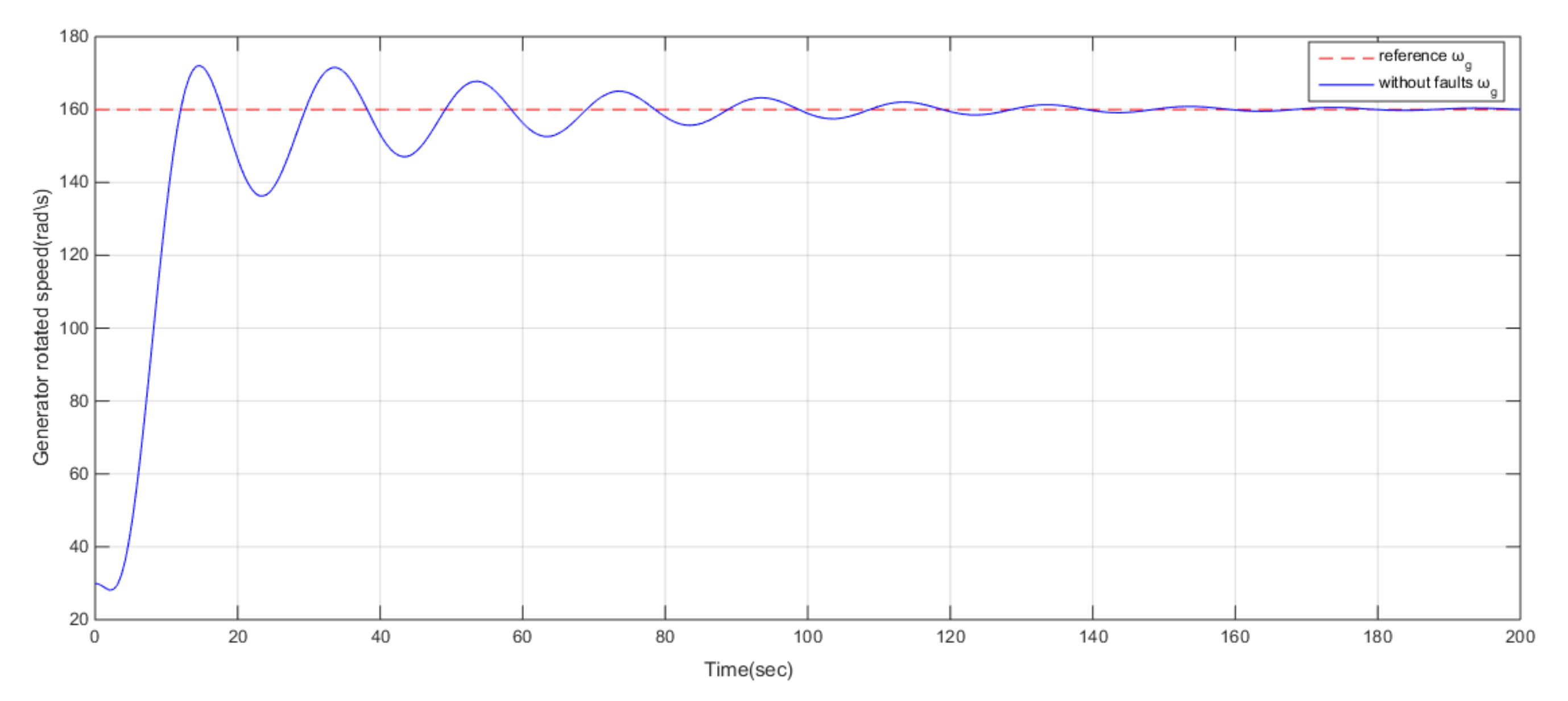
The MPC parameters are selected as follows: the weight matrices of the cost function in Equation (16) are and . The control constraints are and . We consider the generator speed at 160 (rad/s) to maintain the power value of the generator at around 640 kW. For the simulation, we set the initial values as .
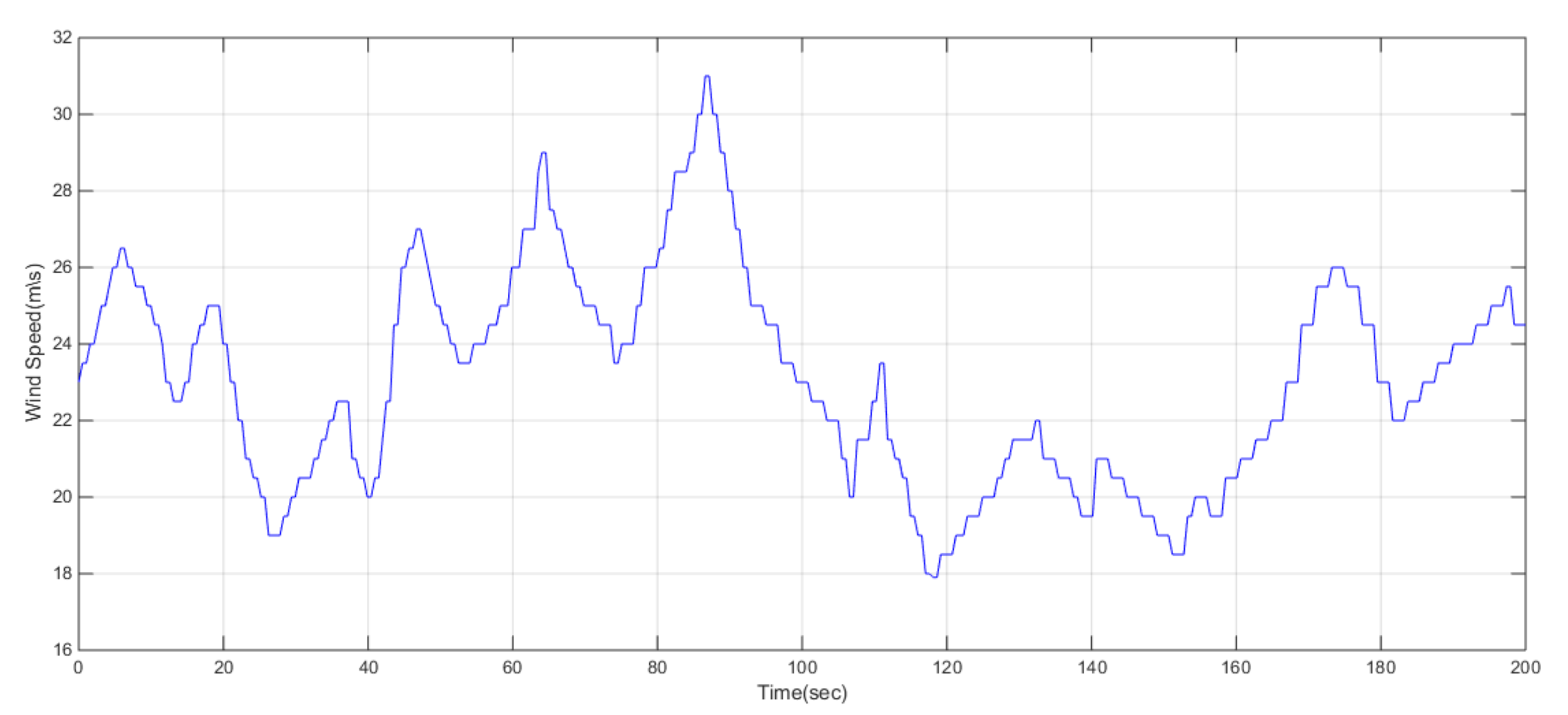
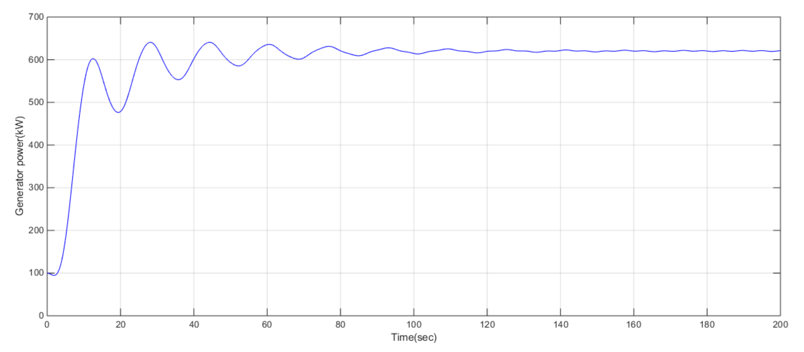
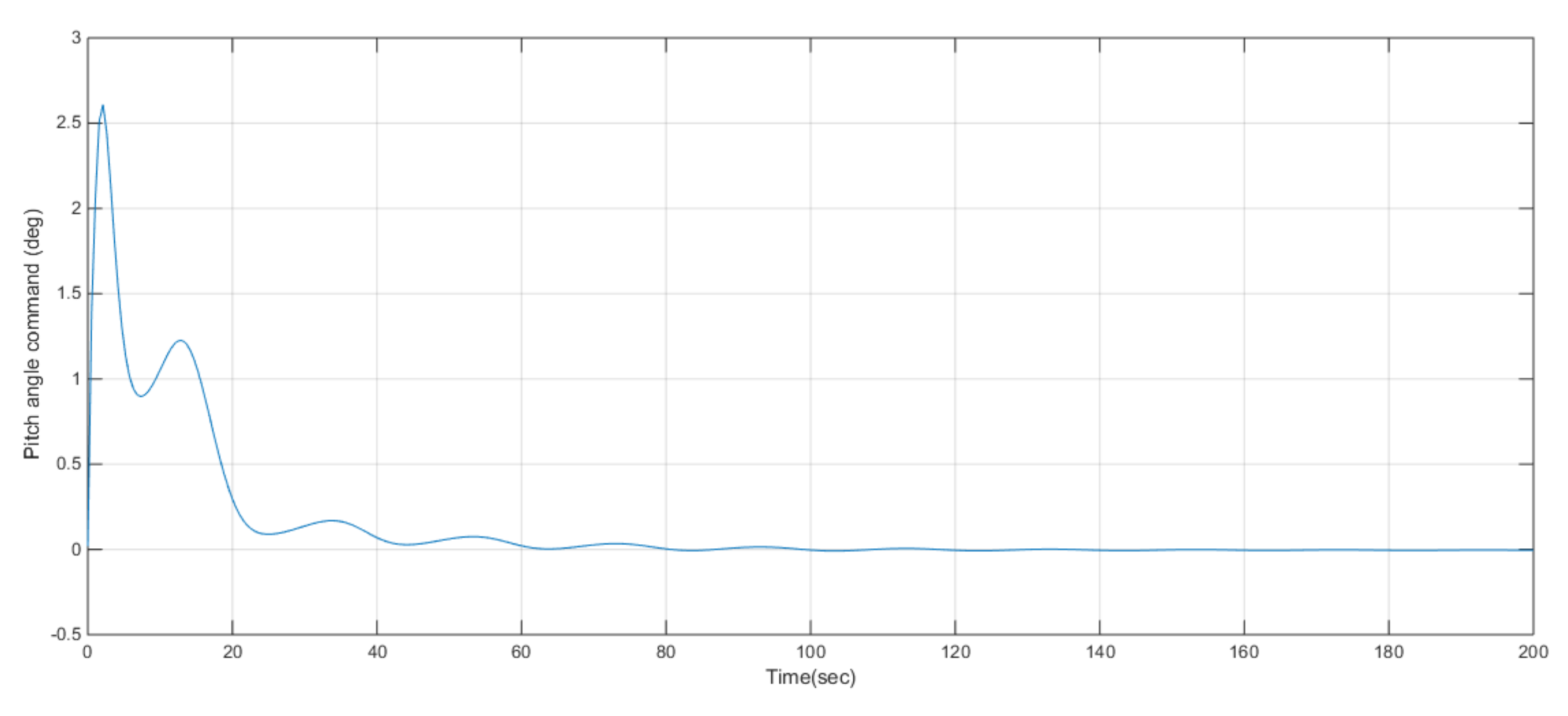
The parameters of the predictive controller are obtained by solving the corresponding LMIs problem. Simulations are carried out with both the generator torque and the pitch and a wind profile [m/s] (see Figure 1). Figure 2 shows that the predicted generator speed can reach 80% of the desired speed at 25 s, which varies between 136 rad/s and 172 rad/s between 0 and 5 s. This is acceptable, since the deviation of remains below 10%. We can also observe that the common objective of regulating the electrical power while restricting the variations of the generator speed is achieved through multivariable pitch and torque control Figure 3. From Figure 4 and Figure 5, we conclude that the RMPC is robust, and has achieved less turbulent control efforts with high accuracy so that the system can track the given reference speed very well.

Figure 1.
Wind speed 17 w 32 (m/s).

Figure 2.
Generator speed predicted without faults.

Figure 3.
predicted without faults.

Figure 4.
Pitch angle control without faults.

Figure 5.
Generator torque control without faults.
From the above simulation results, it is clear that the performance acquired by the RMPC [33] is satisfactory and the multivariable controller tolerates minimizing variations in the speed of the generator and control forces. The combination of these two controls can yield the best results in terms of power regulation. It is also worth noting that:
- The oscillations in the torque speed and generator torque are smoothed, and a good tracking of the nominal power around 610 kW is obtained with the RMPC.
- At the steady regime, the predicted generator rotated speed can reach 95% of the desired speed in 37 s.
- Case 2.
- Simulation with sensor and actuator faults
In this case, it is assumed that the sensor faults in and actuator fault in the wind turbine system contains an additive pitch and generator torque actuators faults and , respectively. The hydraulic pitch systems can have defects on all three blades. These defects are referred to as . Defects considered in the hydraulic system may lead to a change in the dynamics of the system due to a drop in the main line pressure or high air content in the oil. The fault on the torque actuator is mainly due to the internal loop of the power electronics converter which may lead to an offset. This offset can be estimated by a simple comparison between the desired torque (determined by the controller) and the measured torque.
The actuator faults are described as:
The sensor fault for the generator speed is defined as a bounded random signal.
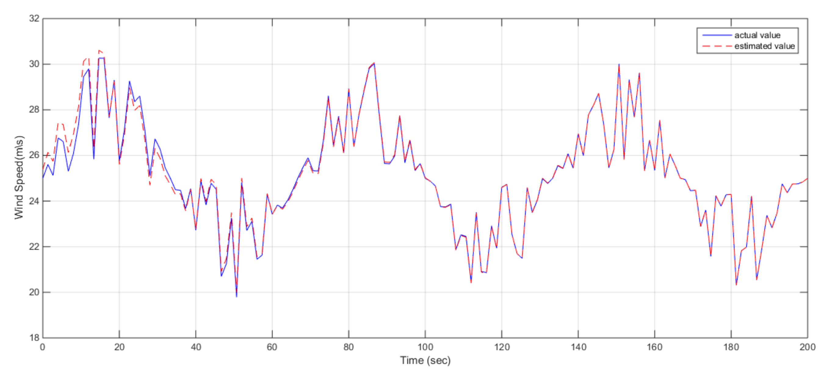
The MPC parameters are selected as follows: the weight matrices of the cost function in Equation (16) are and . The control constraints are , with time delays specified as , the desired value of the generator speed at 160 (rad/s), and the targeted power value of the generator around 640 kW. In the simulations, we set the initial values to be: . In addition, the LMI toolbox is used to deal with the optimization problem described in Equations (39)–(42) at every sampling time. The observer gain matrix and controller gain matrix can are obtained for each sampling time. Simulations are carried out with both the generator torque and the pitch and a wind profile 20 (m/s) (see Figure 6).

Figure 6.
Wind speed disturbances and its estimation.
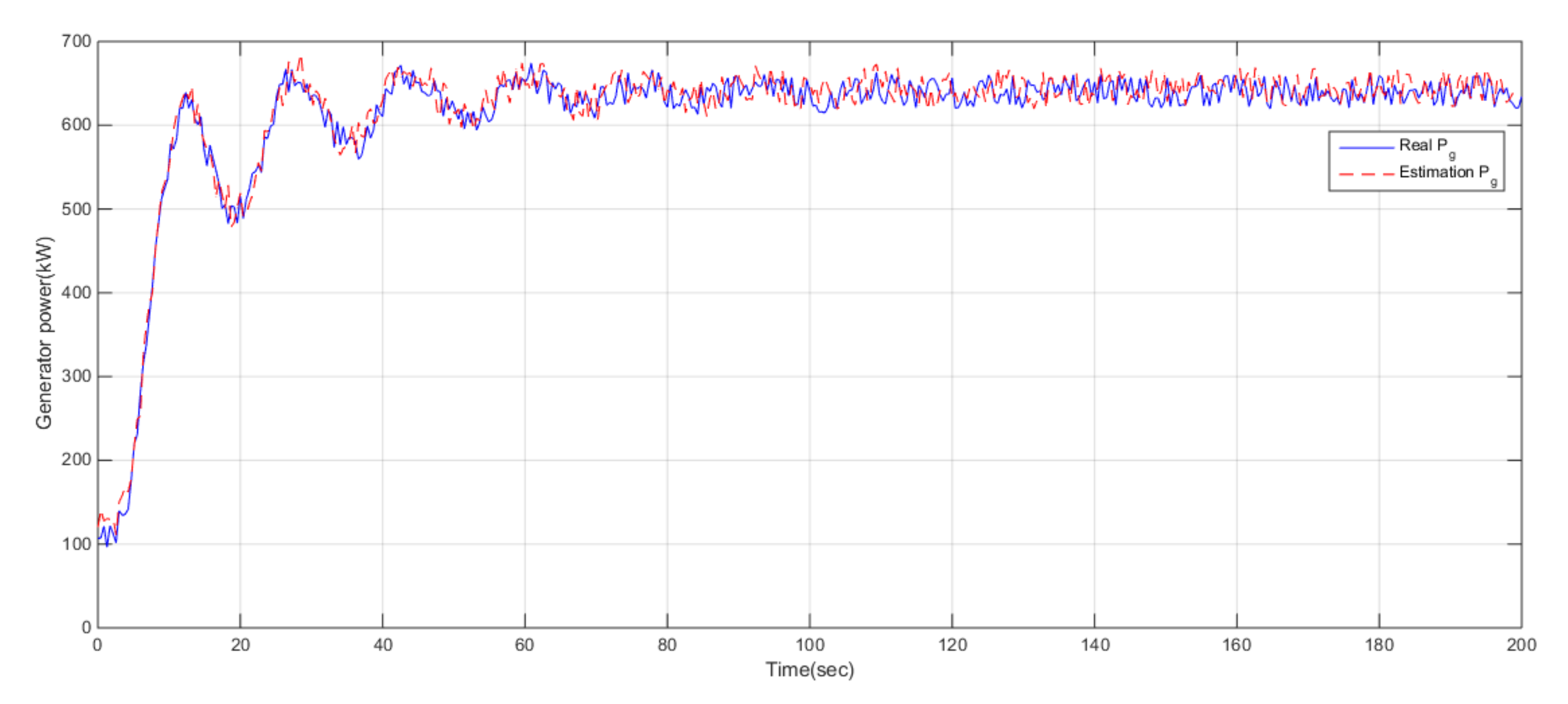
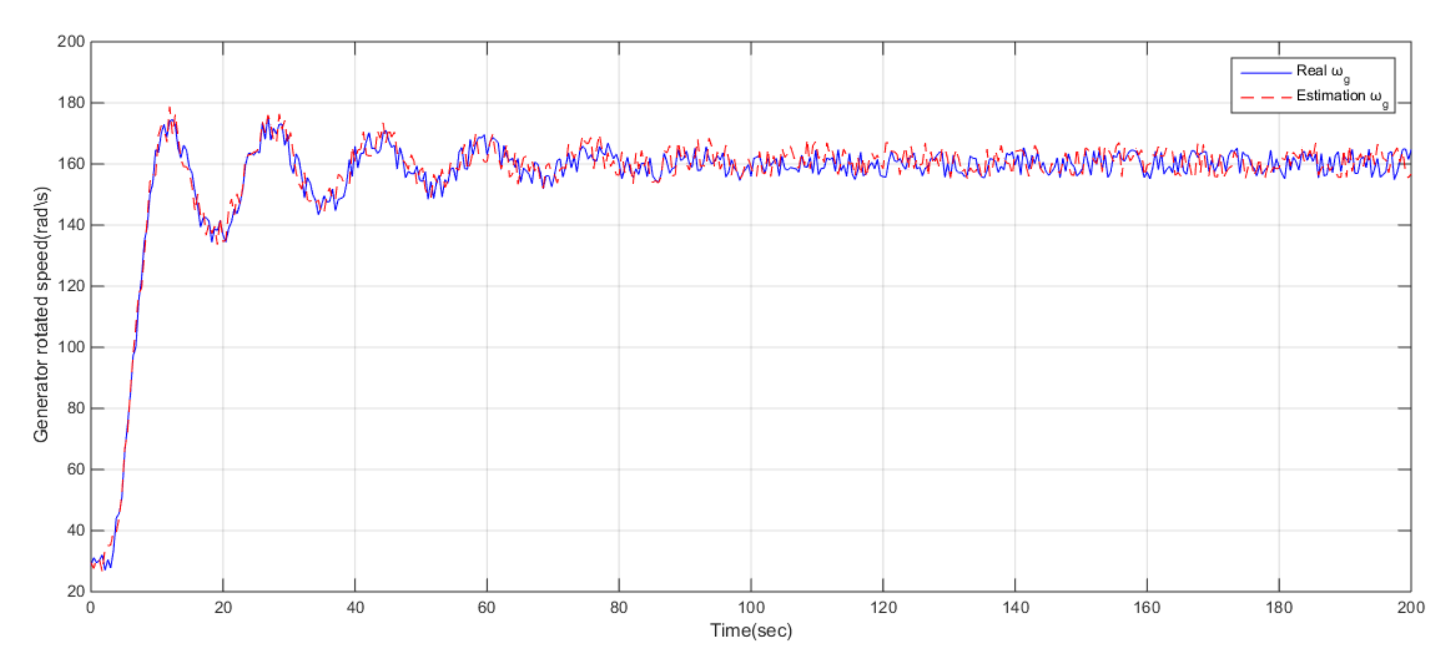
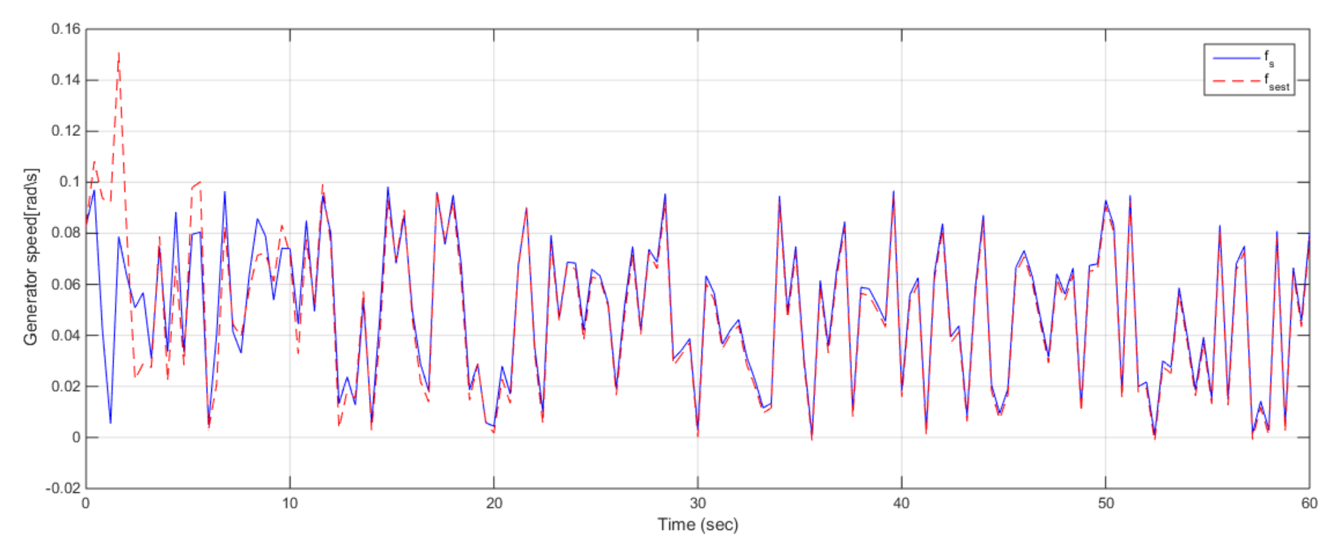
The objective of the proposed FTC approach is to design a control system to guarantee a good trajectory tracking while robust performance is obtained despite the existence of the fault, and with the constraints on the inputs. Figure 6 shows the results of the observer-based fault predictive controller, which allows us to estimate the fictitious wind speed disturbances. Figure 7 and Figure 8 illustrate the temporal responses of the generator power and the generator speed, from which it is apparent that both variables can converge rapidly with the actuator faults and the estimations of the power and speed lead to an excellent estimation performance. Note that the faults have an impact during the transient period in the state change. i.e., even in the presence of faults, the power and speeds can only reach the desired values of 84% at 25 s and 82% at 22 s, respectively.

Figure 7.
with a fault in is present and its estimation.

Figure 8.
with a fault present and its estimation.
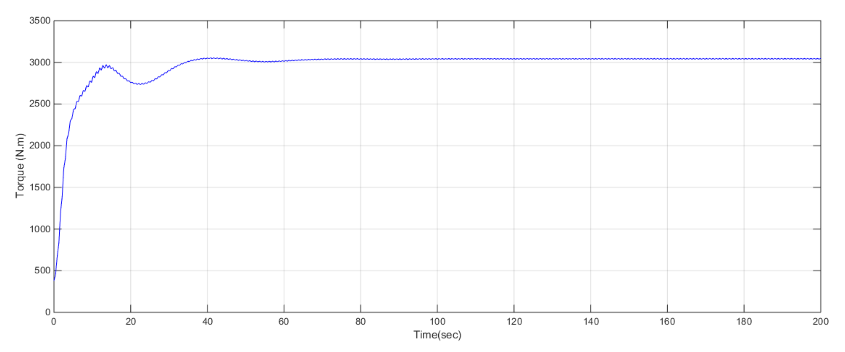
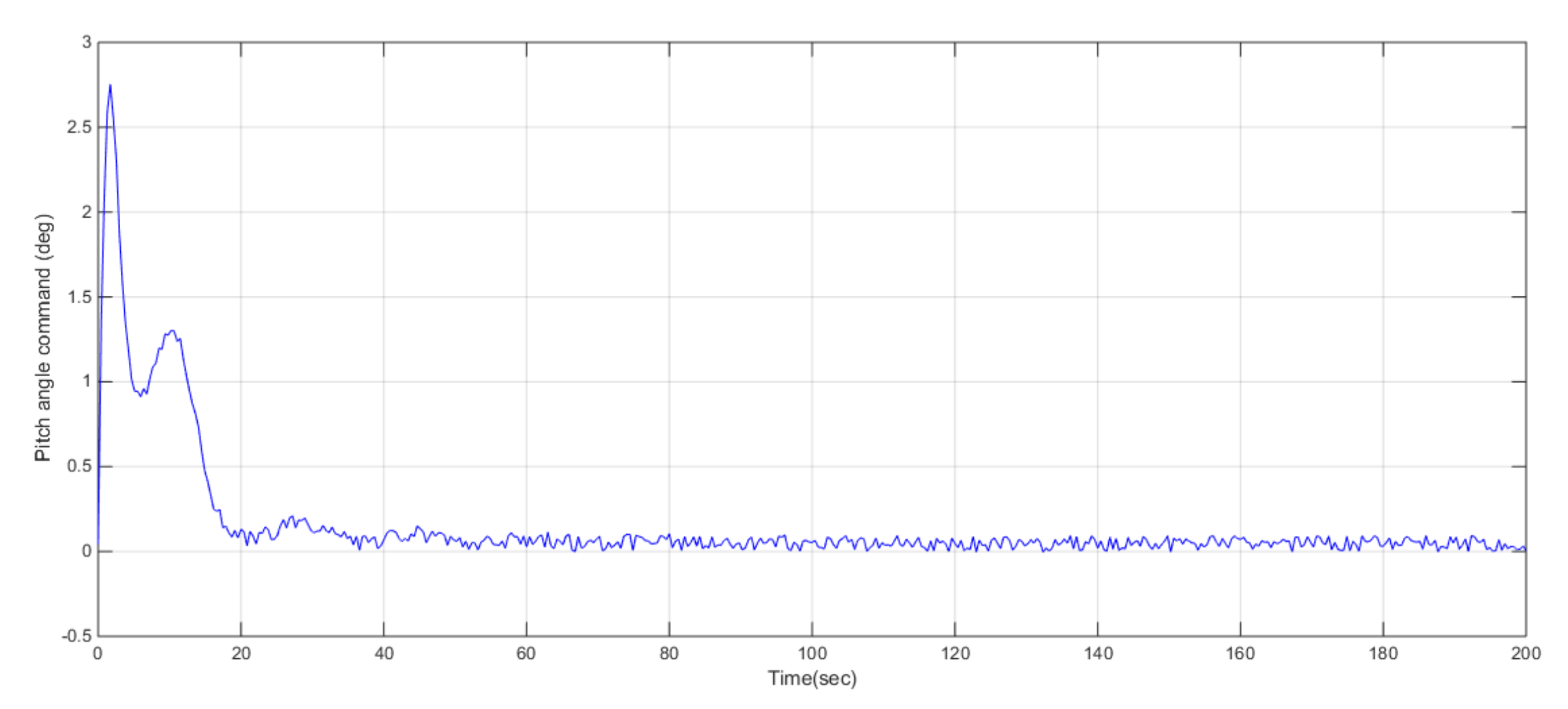
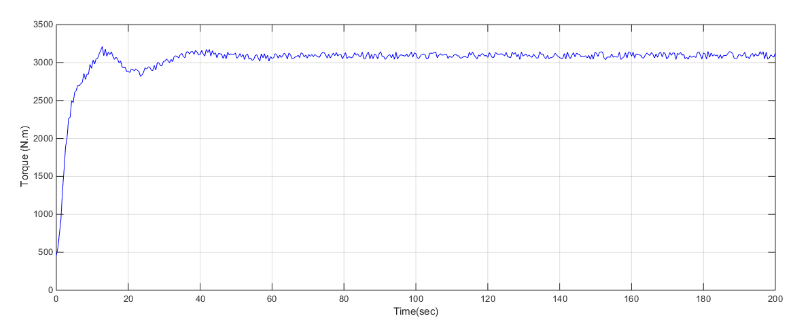
The control inputs, pitch angle, and torque signals are shown in Figure 9, Figure 10 and Figure 11. It is observed that the constraints on the control inputs can be handled by our method, and they do not exceed 3° and 3200 N.m. This meets the requirement of the engineering practice, i.e., the limited control capacity, which is reflected in the minimization of control forces as well as the transient loads experienced by the wind turbine.

Figure 9.
control input with fault.

Figure 10.
with a fault present.

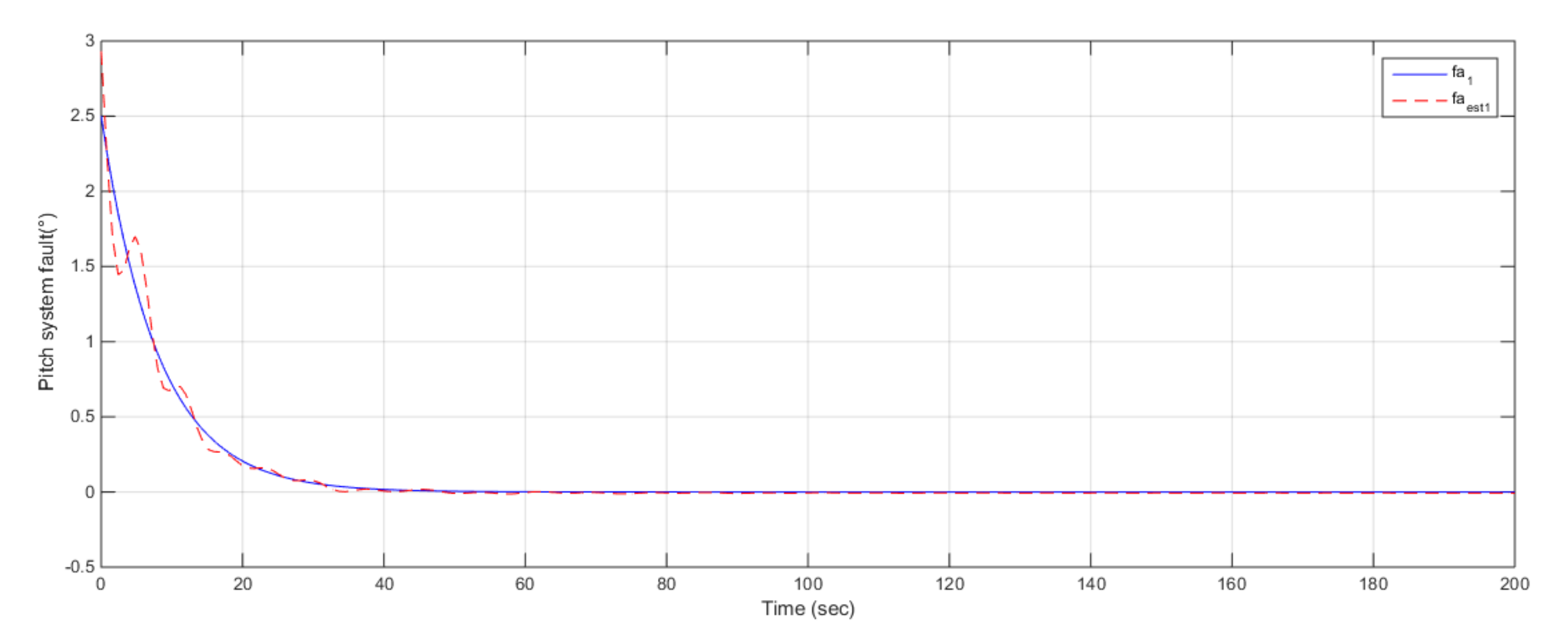
Figure 11.
Pitch system fault and its estimation.
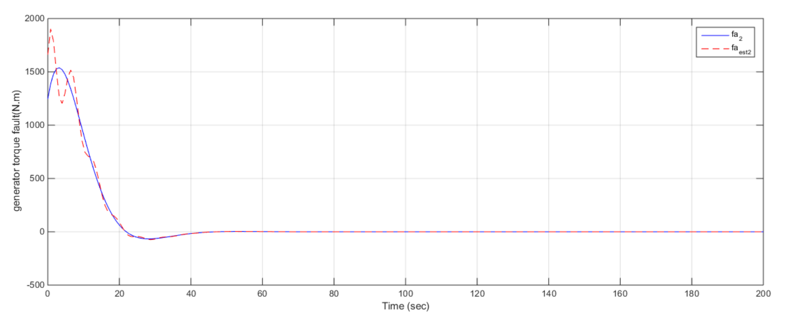
Figure 11, Figure 12 and Figure 13 show the time responses of the actuator/sensor faults signal and their estimations. We can see that the estimation of sensor fault can reach up to 90% of real values within 20 s. It should be highlighted that the robust asymptotic stability of the closed loop system is guaranteed in the case of wind speed disturbances, sensor, and actuator faults. In addition, the tracking values of the generator speed and generator power can reach 95% of the desired values at around 40 s and 50 s respectively. According to the simulation results, we conclude that the system states and fault information can be estimated with acceptable accuracy by using our observer-based fault predictive controller. From all figures, it is noted that the delay effect with the proposed OBRFPC approach is negligible because the computation of the controller is done in a prediction horizon that considers time delays and allows to anticipate and compensate for its effect in advance.

Figure 12.
Generator fault and its estimation.

Figure 13.
Random generator fault and its estimation.
Table 2 shows the root mean square (RMS) error comparison between the proposed OBRFPC approach and the method discussed in [33].

Table 2.
RMS comparison of wind turbine responses with sensor faults.
The comparison describes the RMS errors of the wind turbine responses in terms of suspension stroke, the power produced by the generator, Generator speed, generator torque under generator torque, and random generator faults excitation in the presence of wind disturbances. In addition, Table 2 describes the maximum values reached in power produced by the power generator, generator speed, and generator torque with RMS errors of 95% of the desired values at around 40 s and 50 s, respectively. The results suggested that the proposed robust predictive controller has better performance than the approach discussed in [33] when the system is subject to sensor faults and external disturbances. As can be seen from the error obtained by RMS, the error in the case of the proposed robust approach remains less than 5% of the desired value. This means that the significant fluctuation in blade pitch actuation and energy production, which is due to disturbances and faults in the wind turbine, decreases significantly. On the other hand, the deviation exceeds 15% in the approach cited in [33], which implies instability in energy production [33].
Note that the illustrated performance of the proposed fault predictive controller is due to the following two points.
As a result, the proposed robust predictive control method is well-suited for multivariable systems. In addition, external disturbances and faults in the output channel are already taken into account in the predictive control design procedures, which means that the multivariable control minimizes variations in the generator speed and control forces and the observer can estimate the system states correctly when system suffers from external disturbances and faults. In conclusion, the proposed robust predictive controller has the ability to anticipate any errors caused by external disturbances and actuator/sensor faults and provides reliable control for power regulation while minimizing mechanical loads on the wind turbine structure.
6. Conclusions
In this paper, an observer-based robust predictive control problem in wind turbine systems with time delays subject to actuator faults, sensor faults, and wind speed disturbances is investigated. Based on an augmented system composed of the state variables, actuator fault, and sensor fault, an augmented robust observer is designed and used to estimate states and faults. The main difficulty of the above problem is that the design conditions must satisfy the hard constraints of the system states and inputs and guarantee the system’s stability conditions. Therefore, in the proposed work, the observer design is formulated as an LMI optimization problem. Note that by formulating the main proposed controlling scheme as linear matrix inequalities (LMIs) problem, the infinite time domain “min-max” optimization problems are converted into convex optimization problems, and the sufficient conditions for the existence of this controller and its expression are easily derived. In the numerical example, the augmented robust observer can accurately estimate wind speed disturbances, actuator faults, and sensor faults.in addition, the simulation results show that this approach can effectively guarantee the asymptotical stability of the closed-loop control systems. In future research, we will focus on an extension of the presented approach for the wind turbine with a time-varying delay in the actuator.
Author Contributions
Conceptualization, S.B., A.A., I.B. and F.A.; methodology, S.B., F.A., A.A. and M.C.; validation, S.B., F.A., M.C. and I.B; formal analysis, S.B., A.A., F.A. and I.B.; investigation, S.B., A.A., F.A. and Z.A.B.; writing—original draft preparation, S.B., F.A., R.G., B.N. and M.C.; writing—review and editing S.B., F.A., B.N. and Z.A.B. All authors have read and agreed to the published version of the manuscript.
Funding
This research received no external funding.
Data Availability Statement
Data sharing not applicable. No new data were created or analyzed in this study.
Conflicts of Interest
The authors declare no conflict of interest.
References
- Quadros, M.M.; de Bessa, I.V.; Leite, V.J.S.; Palhares, R.M. Fault tolerant control for linear parameter varying systems: An improved robust virtual actuator and sensor approach. ISA Trans. 2020, 104, 356–369. [Google Scholar] [CrossRef] [PubMed]
- Bououden, S.; Boulkaibet, I.; Chadli, M.; Abboudi, A. A Robust Fault-Tolerant Predictive Control for Discrete-time Linear Systems Subject to Sensor and Actuator faults. Sensors 2021, 21, 2307. [Google Scholar] [CrossRef] [PubMed]
- Tabatabaeipour, S.M.; Stoustrup, J.; Bak, T. Fault-tolerant control of discrete-time LPV systems using virtual actuators and sensors. Int. J. Robust Nonlinear Control 2014, 25, 707–734. [Google Scholar] [CrossRef]
- Rotondo, D.D.; Nejjaria, F.; Puig, V. A virtual actuator and sensor approach for fault tolerant control ofLPV systems. J. Process Control 2014, 24, 203–222. [Google Scholar] [CrossRef]
- Abboudi, A.; Bououden, S.; Chadli, M.; Boulkaibet, I.; Neji, B. Observer-based Fault-Tolerant Predictive Control for LPV systems with Sensor Faults: An Active Car Suspension application. Appl. Sci. 2022, 12, 684. [Google Scholar] [CrossRef]
- Badihi, H.; Zhang, Y.; Hong, H. Wind Turbine Fault Diagnosis and Fault-Tolerant Torque Load Control Against Actuator Faults. IEEE Trans. Control. Syst. Technol. 2015, 23, 1351–1372. [Google Scholar] [CrossRef]
- Sharmila, V.; Rakkiyappan, R.; Joo, Y.H. Fuzzy Sampled-Data Control for DFIG-Based Wind Turbine With Stochastic Actuator Failures, IEEE Transactions on Systems. Man Cybern. Syst. 2021, 51, 2199–2211. [Google Scholar]
- Rahimilarki, R.; Gao, Z.; Zhang, A.; Binns, R. Robust Neural Network Fault Estimation Approach for Nonlinear Dynamic Systems With Applications to Wind Turbine Systems. IEEE Trans. Ind. Inform. 2019, 15, 6302–6312. [Google Scholar] [CrossRef]
- Che, G.; Yu, Z. Neural-network estimators based fault-tolerant tracking control for AUV via ADP with rudders faults and ocean current disturbance. Neurocomputing 2020, 411, 442–454. [Google Scholar] [CrossRef]
- Wu, A.; Zhao, B.; Mao, J.; Wu, B.; Yu, F. Adaptive active fault-tolerant mppt control for wind power generation system under partial loss of actuator effectiveness. Int. J. Electric. Power Energy Syst. 2019, 105, 660–670. [Google Scholar] [CrossRef]
- Yu, D.; Chen, Z.; Xiahou, K.; Li, M.; Ji, T.; Wu, Q. A radically data-driven method for fault detection and diagnosis in wind turbines. Int. J. Electric. Power Energy Syst. 2018, 99, 577–584. [Google Scholar] [CrossRef]
- Odgaard, P.F.; Stoustrup, J.; Kinnaert, M. Fault-Tolerant Control of Wind Turbines: A Benchmark Model. IEEE Trans. Control. Syst. Technol. 2013, 21, 1168–1182. [Google Scholar] [CrossRef]
- Yang, B.; Yu, T.; Shu, H.; Zhang, Y.; Chen, J.; Sang, Y. Passivity-based sliding-mode control design for optimal power extraction of a pmsg based variable speed wind turbine. Renew. Energy 2018, 119, 577–589. [Google Scholar] [CrossRef]
- Liang, X.; Wanga, Q.; Hub, C.; Dong, C. Observer-based H∞fault-tolerant attitude control for satellite with actuator and sensor faults. Aerosp. Sci. Technol. 2019, 95, 105424. [Google Scholar] [CrossRef]
- Shaker, M.S.; Patton, R.J. Active sensor fault tolerant output feedback tracking control for wind turbine systems via T–S model. Eng. Appl. Artif. Intell. 2014, 34, 1–12. [Google Scholar] [CrossRef]
- Zahaf, A.; Bououden, S.; Chadli, M.; Chemachema, M. Robust fault tolerant optimal predictive control of hybrid actuators with time varying delay for industrial robot arm. Asian J. Control 2022, 24, 1–15. [Google Scholar] [CrossRef]
- Wang, L.; Cai, M.; Zhang, H.; Alsaadi, F.; Chen, L. Active Fault-Tolerant Control for Wind Turbine with Simultaneous Actuator and Sensor Faults. Complexity 2017, 2017, 6164841. [Google Scholar] [CrossRef]
- Li, J.; Zhang, D.; Wang, Z. Novel MPC-Based fault tolerant tracking control against sensor faults. Asian J. Control 2020, 22, 841–854. [Google Scholar] [CrossRef]
- Tavakoli, M.M.; Assadian, N. Predictive fault-tolerant control of an all-thruster satellite in 6-DOF motion via neural network model updating. Adv. Space Res. 2018, 61, 1588–1599. [Google Scholar] [CrossRef]
- Shi, H.; Li, P.; Sub, C.; Wang, Y.; Yub, J.; Cao, J. Robust constrained model predictive fault-tolerant control for industrial processes with partial actuator failures and interval time-varying delays. J. Process Control 2019, 75, 187–203. [Google Scholar] [CrossRef]
- Zarcha, G.M.; Puig, V.; Poshtan, J.; Shoorehdeli, M.A. Actuator fault tolerance evaluation approach of nonlinear model predictive control systems using viability theory. J. Process Control 2018, 71, 35–45. [Google Scholar] [CrossRef]
- Luo, Z.; Liu, C.; Liu, S. A Novel Fault Prediction Method of Wind Turbine Gearbox Based on Pair-Copula Construction and BP Neural Network. IEEE Access 2020, 8, 91924–91939. [Google Scholar] [CrossRef]
- Shi, F.; Patton, R. An active fault tolerant control approach to an offshore wind turbine model. Renew. Energy 2015, 75, 788–798. [Google Scholar] [CrossRef]
- Cho, S.; Gao, Z.; Moan, T. Model-based fault detection, fault isolation and fault-tolerant control of a blade pitch system in floating wind turbines. Renew. Energy 2018, 120, 306–321. [Google Scholar] [CrossRef]
- Sanchez, H.E.; Escobet, T.; Puig, V.; Odgaard, P.F. Health-aware model predictive control of wind turbines using fatigue prognosis. Int. J. Adapt. Control. Signal Process. 2017, 32, 614–627. [Google Scholar] [CrossRef]
- Benlahrache, M.A.; Laib, K.; Othman, S.; Sheibat-Othman, N. Fault tolerant control of wind turbine using robust model predictive min-max approach. IFAC-Pap. Line 2017, 50, 9902–9907. [Google Scholar] [CrossRef]
- Jain, T.; Yame, J.J. Fault-tolerant Economic Model Predictive Control for Wind Turbines. IEEE Trans. Sustain. Energy 2019, 10, 1696–1704. [Google Scholar] [CrossRef]
- Hsu, J.Y.; Wang, Y.F.; Lin, K.C.; Chen, M.Y.; Hsu, J.H.Y. Wind Turbine Fault Diagnosis and Predictive Maintenance Through Statistical Process Control and Machine Learning. IEEE Access 2020, 8, 23427–23439. [Google Scholar] [CrossRef]
- Ghanbarpour, K.; Bayat, F.; Jalilvand, A. Dependable power extraction in wind turbines using model predictive fault tolerant control. Electr. Power Energy Syst. 2020, 118, 105802. [Google Scholar] [CrossRef]
- Boyd, S.; El Ghaoui, L.; Feron, V. Balakrishnan, Linear Matrix Inequalities in System and Control Theory; Society for Industrial and Applied Mathematics (SIAM): Philadelphia, PA, USA, 1994; p. 15. [Google Scholar]
- Kothare, M.; Balakrishnan, V.; Morari, M. Robust Constrained Model Predictive Control using Linear Matrix Inequalities. Automatica 1996, 32, 1361–1379. [Google Scholar] [CrossRef]
- Bucolo, M.; Buscarino, A.; Famoso, C.; Fortuna, L.; Frasca, M. Control of imperfect dynamical systems. Nonlinear Dyn. 2019, 98, 2989–2999. [Google Scholar] [CrossRef]
- Bououden, S.; Chadli, M.; Filali, S.; El Hajjaji, A. Fuzzy Model Based Multivariable Predictive Control of a Variable Speed Wind Turbine: LMI approach. Renew. Energy 2012, 37, 434–439. [Google Scholar] [CrossRef]
- Bianchi, F.D.; De Battista, H.; Mantz, R.J. Wind Turbine Control Systems; Springer: Berlin/Heidelberg, Germany, 2006. [Google Scholar]
Disclaimer/Publisher’s Note: The statements, opinions and data contained in all publications are solely those of the individual author(s) and contributor(s) and not of MDPI and/or the editor(s). MDPI and/or the editor(s) disclaim responsibility for any injury to people or property resulting from any ideas, methods, instructions or products referred to in the content. |
© 2023 by the authors. Licensee MDPI, Basel, Switzerland. This article is an open access article distributed under the terms and conditions of the Creative Commons Attribution (CC BY) license (https://creativecommons.org/licenses/by/4.0/).

