Cuttings Bed Height Prediction in Microhole Horizontal Wells with Artificial Intelligence Models

Abstract

Inadequate drill cuttings removal can cause costly problems such as excessive drag, lower rate of penetration, and even mechanical pipe sticking. Cuttings bed height is usually used to evaluate hole-cleaning efficiency in horizontal wells. In this study, artificial intelligence models, including artificial neural network (ANN), support vector regression (SVR), recurrent neural network (RNN), and long short-term memory (LSTM), were employed to predict cuttings bed height in the well-bore. A total of 136 different tests were conducted, and cuttings bed height under different conditions were measured in our previous study. By training four different artificial intelligence models with the experiment data, it was found that the ANN model performed best among other artificial intelligence models. The ANN model outperformed the dimensionless cuttings bed height model proposed in our previous study. Due to the amount of data points, the memory ability of RNN and LSTM models has not been entirely played compared with the ANN model.

1. Introduction

Cuttings are generated after the drill bit breaks the formation rock. Drilling fluids are used to clean cuttings from the bit and transport cuttings from the bottomhole to the surface, in order to avoid regrinding and to improve the rate of penetration (ROP). Due to the interactions between cuttings and cuttings with drilling fluids, drillpipe, and wellbore, solid-liquid flow characteristics are complicated during cuttings transport. A good understanding of cuttings transport characteristics is key to hydraulics optimization, hole cleaning, and safe drilling.

In vertical or low-inclined wells, cuttings will not form a cuttings bed. Cuttings transport characteristics could be adequately evaluated by the ratio between cuttings transport velocity and annulus fluid velocity [1]. When the fluid velocity is large enough to resist gravity, cuttings will be transported to the surface successfully, ensuring effective hole cleaning. Otherwise, cuttings will settle back to the drill bit and induce many accidents, such as excessive drag, lower rate of penetration, and even mechanical pipe sticking.

With the development of directional well drilling, horizontal well drilling, and extended reach well drilling, the hole-cleaning problem has become critical. In directional, horizontal, or extended reach wells, as the wellbore inclination angle increases the radial component of cuttings gravity increases, and cuttings tend to settle towards the lower side of the annulus. Drillpipe eccentricity increases accordingly as the wellbore inclination angle increases. The increased eccentricity will lead to a decrease in fluid velocity on the lower side of the annulus. The combined effect of gravity and low fluid velocity will increase cuttings concentration, and cuttings beds are more easily formed [2]. Poor hole cleaning causes about one-third of pipe-sticking accidents. Apart from pipe sticking, poor hole cleaning could also lead to excessive drill bit wear, decreased ROP, increased equivalent circulating density (ECD), formation fracture, increased drag, torque forces, etc. These problems will eventually increase non-productive time and drilling costs. Therefore, cuttings transport characteristics and hole-cleaning performance should be thoroughly understood to ensure safe and efficient drilling.

Influence factors of cuttings transport could be divided into four categories: operating parameter (annulus fluid velocity, ROP, drill pipe rotation speed), wellbore geometry (wellbore inclination angle, eccentricity, annulus size), drilling fluid property (drilling fluid density, drilling fluid rheology), and cuttings property (cuttings density, cuttings size, cuttings shape) [3,4]. When adjusting these parameters to improve hole-cleaning performance, field engineers should consider the influence degree of these parameters and evaluate the controllable degree of these factors in the field.

The complexity of the cuttings transport process prompts researchers to use different research methods. The research methods of cuttings transport can be divided into three categories: numerical simulation, theoretical model, and experiment.

With the development of numerical simulation technology and computer power, computational fluid dynamics (CFD) has gradually become an effective method to study the cuttings transport process. Numerical simulation does not require an expensive experimental setup and can be used to study cuttings transport characteristics under any condition in the wellbore. The CFD method can obtain the microscopic flow characteristics in the cuttings transport process. The computational cost of CFD is much higher than that of the theoretical model, so the wellbore length for CFD simulation is relatively short, ranging from several to ten meters.

The theoretical model has a broader range of applicability because the actual physical rules are embedded into the model. The previous theoretical model for cuttings transport can be divided into two categories: the critical velocity model and the layer transport model. However, many empirical parameters must be determined based on the experimental results.

Experiment is the most direct and accurate method to reveal the cuttings transport characteristics in the wellbore. The experimental results can be used to verify the accuracy of numerical simulation and determine the coefficients in the theoretical model. Based on the experimental data, empirical, dimensionless, and intelligent models are developed to predict the cuttings transport efficiency. However, the experimental method has its limitations. On the one hand, it is difficult to conduct cuttings transport experiments under all conditions because many factors affect the cuttings transport process. On the other hand, the proposed empirical, dimensionless, or intelligent prediction models using experimental data are not based on physical rules, so applying these models beyond the scope of the laboratory experiment could yield less accurate predictions.

The artificial intelligence model has been widely used in petroleum engineering [5,6,7,8,9,10,11]. Intelligent models for the prediction of cuttings transport efficiency include fuzzy logic (FL), artificial neural network (ANN), genetic algorithm, etc. Ozbayoglu et al. (2002) [12] first developed an intelligent model to predict cuttings bed area. The accuracy of intelligent prediction models depends on the quality of training data. An intelligent prediction model can effectively deal with imprecise and uncertain problems. Researchers have applied intelligent models to predict cuttings terminal settling velocity, cuttings concentration [13], and cuttings bed height [12,14], as shown in Table 1. It should be noted that there are more than two hundred published papers about cuttings transport; however, only those papers about cuttings transport and the research methodology based on an artificial intelligence model are summarized here.

Table 1. Summarization of intelligent models for the prediction of cuttings transport efficiency.

Authors	Model	Model Input		Predicted Parameter
		Number	Input Parameters
Ozbayoglu et al. (2002) [12]	ANN	3	Cuttings injection concentration, Reynolds number, Froude number	Cuttings bed area ratio
Rooki et al. (2014) [15]; Rooki and Rakhshkhorshid (2017) [16]	ANN, RBFN	6	Foam velocity, Foam quality, Pressure, Temperature, Drillpipe rotation speed, Eccentricity	Cuttings concentration
Ulker and Sorgun (2016) [14]	kNN, SVM, LR, ANN	4	Fluid velocity, Drillpipe rotation speed, ROP, Wellbore inclination angle	Cuttings bed area ratio
Al-Azani et al. (2018) [17]; Al-Azani et al. (2019) [13]	SVM, ANN	9	Drilling fluid density, Fluid yield point stress, Fluid plastic viscosity, Wellbore inclination angle, Eccentricity, ROP, Fluid flow rate, Drillpipe rotation speed, Temperature	Cuttings concentration
Chowdhury and Hovda (2022) [18]	FL	11	Annulus size, Wellbore inclination angle, Eccentricity, Temperature, Drilling fluid density, Apparent viscosity, Cuttings size, Cuttings density, Drilling fluid flow rate, Drillpipe rotation speed, ROP	Cuttings concentration

However, it was found that there are few studies to predict cuttings bed height with an artificial intelligence model. Therefore, this study aims to predict cuttings bed height with an artificial intelligence model other than mechanistic or empirical models. Four different artificial intelligence methods were developed to predict cuttings bed height in a microhole horizontal wellbore, and their predicted accuracies are compared.

2. Artificial Intelligence Models

Four different artificial intelligence models are used to predict cuttings bed height in a microhole horizontal wellbore. They are Artificial neural network (ANN), Support vector regression (SVR), Recurrent neural network (RNN), and Long short-term memory (LSTM).

2.1. Artificial Neural Network (ANN)

Each layer in the ANN model contains several neurons, as shown in Figure 1. The exact relationship between input and output is not required. It only needs to know the non-constant factors causing output changes. By repeated training of the network, the connection weights are adjusted step by step. Therefore, compared with traditional data processing methods, the ANN model has apparent advantages in processing fuzzy, random, and nonlinear data, especially for large-scale, complex structure, and unclear information systems.

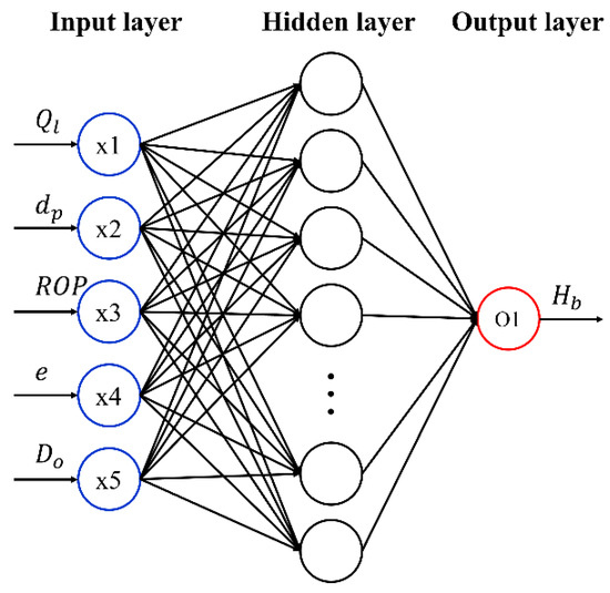
Figure 1. The schematic of the ANN model ($Q_l$ is the flow rate of drilling fluids (${\mathrm{m}}^3/\mathrm{s}$), $d_p$ is the cuttings diameter ($\mathrm{m}$), $ROP$ is the rate of penetration ($\mathrm{m}/\mathrm{s}$), $e$ is the eccentricity, $D_o$ is the wellbore diameter ($\mathrm{m}$), $H_b$ is the cuttings bed height ($\mathrm{m}$)).

2.2. Support Vector Regression (SVR)

Support vector regression (SVR) is a vital application branch of Support vector Machine (SVM). SVM is a classifier defined on the feature space with the most considerable interval. It solves the separated hyperplane that can correctly divide the dataset, and has the most significant geometric interval. It is mainly used to solve the binary classification problem. Unlike SVM, SVR is a fitting formula that minimizes the gap between the farthest sample points of the hyperplane and is mainly used for regression fitting.

2.3. Recurrent Neural Network (RNN)

Recurrent neural network (RNN) is a chain-linked artificial neural network with a memory function, whose internal states can display dynamic temporal behavior, as shown in Figure 2. RNN is used initially to describe the relationship between the current output information and the previous information in a sequence, and is mainly used for processing and predicting sequence data. It can transversely transfer data information between neurons and partially express the correlation between data, that is, its hidden layer nodes are interconnected, and the input of the hidden layer not only contains the input characteristics, but also the output value of the hidden layer in the last time step.

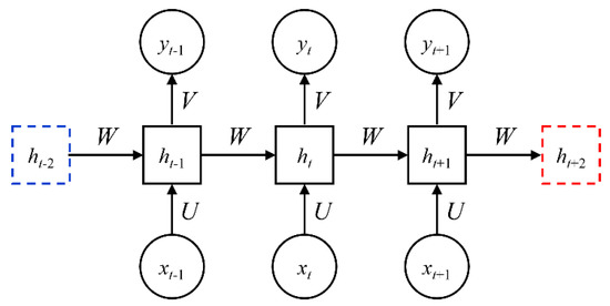
Figure 2. The schematic of the RNN model.

2.4. Long Short-Term Memory (LSTM)

Long short-term memory (LSTM) is a variant of RNN. The hidden layer of ordinary RNN has only one hidden state, $h$, which is very sensitive to short-term input information. However, compared with ordinary RNN, LSTM adds the unit state, $c$, in the structure of the recurrent core, which is responsible for storing the long-term state, so that LSTM can learn long-term dependent information, as shown in Figure 3.

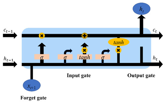
Figure 3. The schematic of the LSTM model.

Among these four artificial intelligence models, ANN has apparent advantages in processing fuzzy, random, and nonlinear data, especially for large-scale, complex structure, and unclear information systems. RNN can adopt the temporal dependencies of both short and long term. Compared to ANN, LSTM is capable of processing not only the single data point, but also the entire sequence of prediction by holding the information of the previous inputs for an amount of time. SVR takes advantages of both regression and SVM. SVR allows more flexibility to define the maximum acceptable error rate in the model.

3. Cuttings Transport Experiment

The experimental setup of cuttings transport includes a 6-m long test section, fluid tank, fluid pump, cuttings injection device, and cuttings/fluid separator. As shown in Figure 4 and Table 2, a total of 136 experimental data were recorded under different flow rate, cuttings diameter, rate of penetration, eccentricity, and wellbore diameter conditions. During the experiment, first, start the drilling fluid pump to obtain the desired flow rate, then inject cuttings into the wellbore with a constant mass flow rate. Afterwards, measure the cuttings bed height at different locations along the wellbore. Based on the experimental data, a dimensionless prediction model for cuttings bed height was developed. Details of the cuttings transport experiment can be obtained from our previous paper [19].

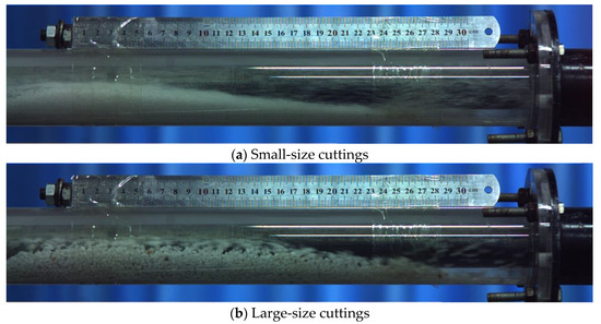
Figure 4. Cuttings transport experiment for cuttings with different sizes.

Table 2. Test matrix for cuttings transport experiments.

Parameter	Range
$\mathrm{Flow} \mathrm{rate} ({\mathrm{m}}^3/\mathrm{s})$	0.00058, 0.00063, 0.00068, 0.00073, 0.00078
$\mathrm{Cuttings} \mathrm{size} \left(\mathrm{m}\right)$	0.0003, 0.0006, 0.0012, 0.0050
$\mathrm{Rate} \mathrm{of} \mathrm{penetration} (\mathrm{m}/\mathrm{s})$	0.00211, 0.00256, 0.00319, 0.00425, 0.00636
Eccentricity	0.0, 0.2, 0.4, 0.6, 0.8
$\mathrm{Wellbore} \mathrm{diameter} \left(\mathrm{m}\right)$	0.04, 0.05, 0.06, 0.08

Figure 5 shows the density estimation and box plot of all the input features for the cuttings transport efficiency dataset, which provides insightful information about the distribution and statistical parameters of the dataset. In our dataset, the flow rate ranges from 0.00058 to 0.00078 ${\mathrm{m}}^3/\mathrm{s}$, the cuttings diameter ranges from 0.0003 to 0.005 $\mathrm{m}$, the rate of penetration ranges from 0.00211 to 0.00256 $\mathrm{m}/\mathrm{s}$, eccentricity ranges from 0 to 0.8, and the wellbore diameter ranges from 0.04 to 0.08 $\mathrm{m}$.

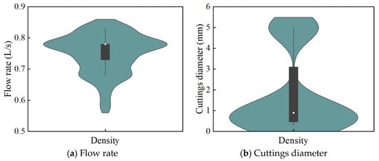
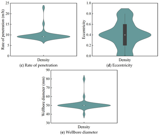
Figure 5. Density distribution and box plot of all the input features for the cuttings bed height prediction (a) flow rate, (b) cuttings diameter, (c) rate of penetration, (d) eccentricity, (e) wellbore diameter).

4. Results and Discussion

Taking the development of the ANN model as an example, the development processes of the other three artificial intelligence models are provided in Appendix A section. The data set is divided into a train set and a test set. The train set is used to establish the weights and deviations in the ANN model, and the test set is used to independently test the prediction ability and reliability of the ANN model. Generally, the trial-and-error method is applied to determine the proportion of different data sets. In this paper, referring to previous studies, the proportion of data points in two data sets is 80% (train set) and 20% (test set). It is generally accepted that the ANN performs best when they are within the range of their train data. In other words, the data used for training and testing must represent the same population. Since the input and output parameters differ in the order of magnitude, all the input variables are converted into values between 0 and 1. The most commonly used ANN model structure is a three-layer model, usually composed of the input layer, hidden layer, and output layer. The ANN model with one hidden layer is the simplest and most common. Though increasing the number of the hidden layer could improve the ANN performance, it could also lead to the overfitting problem when the data set is not large enough. Therefore, the ANN model with one hidden layer is used in this study. There are five nodes in the input layer. Each node corresponds to an input parameter that affects the cuttings bed height, namely, flow rate, cuttings diameter, rate of penetration, eccentricity, and wellbore diameter. The output layer has one node, namely, the cuttings bed height. The architecture of the ANN model is shown in Figure 1.

The configuration and parameters used to train the ANN model are summarized in Table 3. The learning rate affects the speed at which the ANN model arrives at the minimum solution. The loss function is used to quantify the difference between the expected results and the results predicted by the ANN model. The activation function is used to determine the output of the ANN model. That is, it determines whether the neuron should be activated or not. Early stopping is training on the train data set, but stop training while the performance on the validation data set begins to decrease. An epoch means training the neural network with all the training data for one cycle.

Table 3. ANN configuration and parameters used to train ANN model.

Parameter Name	Parameter Value
Learning rate	0.001
Loss function	MSE
Activation function	ReLU for hidden layer, Simoid for output layer
Early stopping	No
Epoch	1000

The number of nodes in the hidden layer is determined by minimizing the difference between predicted and measured settling velocity. Based on the calculation results, it was found that when the number of nodes in the hidden layer is 8, the ANN model performs best. And the average absolute relative errors in the train set and test set are 4.21% and 5.12%, respectively.

The root mean square error (RMSE), average absolute error (AAE), and average absolute percent error (AAPE) between measured and predicted cuttings bed height are compared for these four artificial intelligence models.

Root mean square error (RMSE):

$$\mathrm{RMSE}=\sqrt{\frac{1}{n}{\displaystyle \sum _{i=1}^n{\left[{\widehat{Y}}_i-Y_i\right]}^2}}$$

(1)

Average absolute error (AAE):

$$\mathrm{AAE}=\frac{1}{n}{\displaystyle \sum _{i=1}^n\left|{\widehat{Y}}_i-Y_i\right|}$$

(2)

Average absolute percent error (AAPE):

$$\mathrm{AAPE}=\frac{1}{n}{\displaystyle \sum _{i=1}^n\left|\frac{{\widehat{Y}}_i-Y_i}{Y_i}\right|}$$

(3)

where, ${\widehat{Y}}_i$ is the predicted cuttings bed height, $Y_i$ is the measured cuttings bed height, $n$ is the total number of the experimental data.

Figure 6 compares the measured cuttings bed height and predicted cuttings bed height with the ANN model. The RMSE, AAE, and AAPE of the ANN model are 1.069, 0.794, and 4.66%, respectively. It was found that most of the data points are within the ±15% error margins, thus, the ANN model could provide satisfactory prediction results.

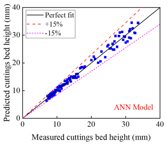
Figure 6. Measured cuttings bed height and predicted cuttings bed height with the ANN model.

Figure 7 compares the measured cuttings bed height and predicted cuttings bed height with the SVR model. The RMSE, AAE, and AAPE of the SVR model are 2.674, 1.556, and 12.32%, respectively. About 1/3 of all the data points are outside the ±15% error margins.

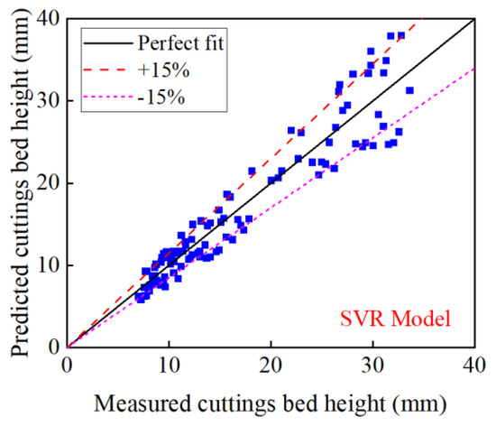
Figure 7. Measured cuttings bed height and predicted cuttings bed height with the SVR model.

Figure 8 compares the measured cuttings bed height and predicted cuttings bed height with the RNN and LSTM models. The RMSE, AAE, and AAPE of the RNN model are 1.741, 1.356, and 8.12%, respectively. The RMSE, AAE, and AAPE of the LSTM model are 1.955, 2.100, and 9.54%, respectively. It was found that most of the data points are within the ±15% error margins. The prediction accuracies of RNN and LSTM models are better than that of the SVR model, but worse than that of the ANN model.

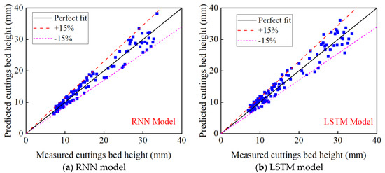
Figure 8. Measured cuttings bed height and predicted cuttings bed height with the RNN and LSTM models (a) RNN model, (b) LSTM model).

The performance results of four different artificial intelligence models are summarized in Table 4. It was found that the ANN model outperforms the other models.

Table 4. Comparison of predicted accuracy for different artificial intelligence models.

Model	RMSE	AAE	AAPE
Artificial Neural Network (ANN)	1.069	0.794	4.66%
Support Vector Regression (SVR)	2.674	1.556	12.32%
Recurrent Neural Network (RNN)	1.741	1.356	8.12%
Long Short-Term Memory (LSTM)	1.955	2.100	9.54%

RNN and LSTM are best for time series problems. The LSTM model considers long-term dependencies and evaluates new values after understanding the whole series pattern, whereas the SVR model considers each row as a sample for training data and predicts the outcome, and will not consider the previous patterns. The reason that the ANN model performs best is because there are only 136 sets of data in the dataset, with a small number of data points; the memory ability of RNN and LSTM models has not been entirely played. Considering the more abundant data accumulated in the field drilling process, the LSTM model with long-term memory capability has more advantages than the ANN model.

The following equation is used to evaluate the relative importance of the input variables [20,21], which is based on the connection weights of the ANN model, as shown in Equation (4).

$$R{I}_j=\frac{{\displaystyle {\sum }_{m=1}^{m=N_h}\left[\left(\frac{\left|W_{jm}^{ih}\right|}{{\displaystyle {\sum }_{k=1}^{k=N_i}\left|W_{km}^{ih}\right|}}\right)\left|W_{mn}^{ho}\right|\right]}}{{\displaystyle {\sum }_{k=1}^{k=N_i}\left\{{\displaystyle {\sum }_{m=1}^{m=N_h}\left(\left|W_{km}^{ih}\right|/{\displaystyle {\sum }_{k=1}^{k=N_i}\left|W_{km}^{ih}\right|}\right)\times \left|W_{mn}^{ho}\right|}\right\}}}$$

(4)

where, $R{I}_j$ is the relative importance of the jth input variable, $N_i$ is the input neuron number, $N_h$ is the hidden neuron number, $W$ is the connection weight, the superscript $i$ represents the input layer, $h$ represents the hidden layer, $o$ represents output layer, the subscripts $k$ represents the input neuron, $m$ represents the hidden neuron, $n$ represents the output neuron.

Here is the calculated relative importance of the input variables is shown in Table 5 and Figure 9. The drilling fluid flow rate is the primary parameter affecting cuttings transport efficiency because the force acting on the cuttings significantly increases as the flow rate increases. Wellbore diameter is another important variable affecting cuttings transport efficiency, since the flow rate decreases as the wellbore diameter increases. Rate of penetration has a moderate effect on the cuttings transport efficiency because the rate of penetration directly affects the amount of cuttings injected into the wellbore. The effects of cuttings size and eccentricity are relatively small compared with other variables.

Table 5. Relative importance of the input variables.

Input Variable	Flow Rate	Cuttings Size	Rate of Penetration	Eccentricity	Wellbore Diameter
Relative importance	0.314	0.131	0.198	0.115	0.242

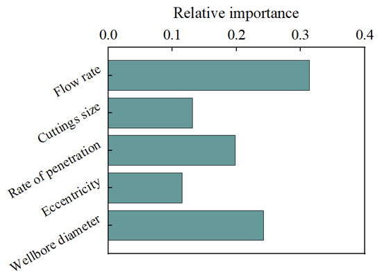
Figure 9. The relative importance of the input variable.

The predicted results of the ANN model are also compared with the dimensionless model predicted by Song et al. (2017) [19], as shown in Equation (5). The AAPE of the dimensionless cuttings bed height model is 9.77%, as shown in Figure 10. In other words, the ANN model performs better than the dimensionless cuttings bed height model.

$$H=m_1·{\Pi }_2^{m_2}\left[{\Pi }_3+m_3·\ln \left({\Pi }_3\right)\right]{\Pi }_4^{m_4}{\left(1+m_5·{\Pi }_5\right)}^{n_5}{\Pi }_6^{m_6}$$

(5)

where, $H$ is the dimensionless cuttings bed height, ${\Pi }_2$ is the Reynolds number, ${\Pi }_3$ is the dimensionless cuttings diameter, ${\Pi }_4$ is the dimensionless cuttings injection rate, ${\Pi }_5$ is eccentricity, ${\Pi }_6$ is the drillpipe/wellbore diameter ratio, $m_1~m_6$ and $n_5$ are fitting parameters, as shown in Table 6.

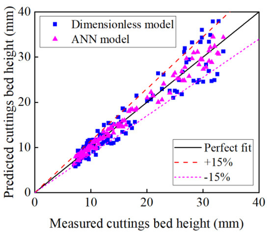
Figure 10. Comparison of predicted results of ANN and dimensionless cuttings bed height models.

Table 6. Fitting parameters for the dimensionless model of cuttings bed height.

${\mathit{m}}_1$	${\mathit{m}}_2$	${\mathit{m}}_3$	${\mathit{m}}_4$	${\mathit{m}}_5$	${\mathit{n}}_5$	${\mathit{m}}_6$
17,059	−0.851	−0.075	0.459	−0.831	0.047	−0.453

5. Conclusions

This study used four artificial intelligence models including ANN, SVR, RNN, LSTM to predict cuttings bed height inside the annulus. A total of 136 experimental data were used as the dataset to test artificial intelligence models.

(1) The ANN model performed best among other artificial intelligence models.

(2) Based on the relative importance analysis of the input variables, it was found that the order of the importance of these variables is: flow rate, wellbore diameter, rate of penetration, cuttings size, and eccentricity.

(3) The ANN model also outperformed the dimensionless cuttings bed height model proposed by Song et al. (2017) [19].

(4) Due to the amount of the data points, the memory ability of RNN and LSTM models has not been fully played compared with the ANN model.

References

- Iyoho, A.W.; Horeth, J.M.; Veenkant, R.L. A computer model for hole-cleaning analysis. J. Pet. Technol. 1988, 40, 1183–1192. [Google Scholar] [CrossRef]
- Avila, R.J.; Pereira, E.J.; Miska, S.Z.; Takach, N.E.; Saasen, A. Correlations and Analysis of Cuttings Transport with Aerated Fluids in Deviated Wells. SPE Drill. Complet. 2008, 23, 132–141. [Google Scholar] [CrossRef]
- Busch, A.; Werner, B.; Johansen, S.T. Cuttings Transport Modeling—Part 2: Dimensional Analysis and Scaling. SPE Drill. Complet. 2020, 35, 69–87. [Google Scholar] [CrossRef]
- Clark, R.K.; Bickham, K.L. A mechanistic model for cuttings transport. In Proceedings of the SPE Annual Technical Conference and Exhibition, New Orleans, LO, USA, 25–28 September 1994. [Google Scholar]
- Mohaghegh, S.D. Recent developments in application of artificial intelligence in petroleum engineering. J. Pet. Technol. 2005, 57, 86–91. [Google Scholar] [CrossRef]
- Farahani, M.V.; Nabi-Bidhendi, M.; Khoshdel, H.; Torabi, S. Applying neuro-fuzzy model to predict reservoir properties from seismic attributes—A case study in an oil field in Iran. In Proceedings of the 71st EAGE Conference and Exhibition incorporating SPE EUROPEC, Amsterdam, The Netherlands, 8–11 June 2009. [Google Scholar]
- Farahani, M.V.; Nabi-Bidhendi, M.; Khoshdel, H. Applying local linear neuro-fuzzy model to predict a well log from other well logs. In Proceedings of the 72nd EAGE Conference and Exhibition incorporating SPE EUROPEC 2010, Barcelona, Spain, 14–17 June 2010. [Google Scholar]
- Farahani, M.V.; Shams, R.; Jamshidi, S. A Robust Modeling Approach for Predicting the Rheological Behavior of Thixotropic Fluids. In Proceedings of the 80th EAGE Conference and Exhibition, Copenhagen, Denmark, 11–14 June 2018. [Google Scholar] [CrossRef]
- Rahmanifard, H.; Plaksina, T. Application of artificial intelligence techniques in the petroleum industry: A review. Artif. Intell. Rev. 2019, 52, 2295–2318. [Google Scholar] [CrossRef]
- Norouzi, S.; Nazari, M.; Farahani, M.V. A Novel Hybrid Particle Swarm Optimization-Simulated Annealing Approach for CO2-Oil Minimum Miscibility Pressure (MMP) Prediction. In Proceedings of the 81st EAGE Conference and Exhibition, London, UK, 3–6 June 2019. [Google Scholar] [CrossRef]
- Kuang, L.; Liu, H.; Ren, Y.; Luo, K.; Shi, M.; Su, J.; Li, X. Application and development trend of artificial intelligence in petroleum exploration and development. Pet. Explor. Dev. 2021, 48, 1–14. [Google Scholar] [CrossRef]
- Ozbayoglu, E.M.; Miska, S.Z.; Reed, T.; Takach, N. Analysis of bed height in horizontal and highly-inclined wellbores by using artificial neural networks. In Proceedings of the SPE International Thermal Operations and Heavy Oil Symposium and International Horizontal Well Technology Conference, Calgary, AB, Canada, 4–7 November 2002. [Google Scholar]
- Al-Azani, K.; Elkatatny, S.; Ali, A.; Ramadan, E.; Abdulraheem, A. Cutting concentration prediction in horizontal and deviated wells using artificial intelligence techniques. J. Pet. Explor. Prod. Technol. 2019, 9, 2769–2779. [Google Scholar] [CrossRef]
- Ulker, E.; Sorgun, M. Comparison of computational intelligence models for cuttings transport in horizontal and deviated wells. J. Pet. Sci. Eng. 2016, 146, 832–837. [Google Scholar] [CrossRef]
- Rooki, R.; Ardejani, F.D.; Moradzadeh, A. Hole Cleaning Prediction in Foam Drilling Using Artificial Neural Network and Multiple Linear Regression. Geomaterials 2014, 4, 47–53. [Google Scholar] [CrossRef]
- Rooki, R.; Rakhshkhorshid, M. Cuttings transport modeling in underbalanced oil drilling operation using radial basis neural network. Egypt. J. Pet. 2017, 26, 541–546. [Google Scholar] [CrossRef]
- Al-Azani, K.H.; Elkatatny, S.; Abdulraheem, A.; Mahmoud, M.; Ali, A. Prediction of Cutting Concentration in Horizontal and Deviated Wells Using Support Vector Machine. In Proceedings of the SPE Kingdom of Saudi Arabia Annual Technical Symposium and Exhibition, Dammam, Saudi Arabia, 23–26 April 2018. [Google Scholar] [CrossRef]
- Chowdhury, D.; Hovda, S. Estimation of downhole cuttings concentration from experimental data—Comparison of empirical and fuzzy logic models. J. Pet. Sci. Eng. 2022, 209, 109910. [Google Scholar] [CrossRef]
- Song, X.; Xu, Z.; Wang, M.; Li, G.; Shah, S.N.; Pang, Z. Experimental Study on the Wellbore-Cleaning Efficiency of Microhole-Horizontal-Well Drilling. SPE J. 2017, 22, 1189–1200. [Google Scholar] [CrossRef]
- Elmolla, E.S.; Chaudhuri, M.; Eltoukhy, M.M. The use of artificial neural network (ANN) for modeling of COD removal from antibiotic aqueous solution by the Fenton process. J. Hazard. Mater. 2010, 179, 127–134. [Google Scholar] [CrossRef] [PubMed]
- Ghorbani, M.A.; Khatibi, R.; Hosseini, B.; Bilgili, M. Relative importance of parameters affecting wind speed prediction using artificial neural networks. Arch. Meteorol. Geophys. Bioclimatol. Ser. B 2013, 114, 107–114. [Google Scholar] [CrossRef]
Publisher’s Note: MDPI stays neutral with regard to jurisdictional claims in published maps and institutional affiliations. |
© 2022 by the authors. Licensee MDPI, Basel, Switzerland. This article is an open access article distributed under the terms and conditions of the Creative Commons Attribution (CC BY) license (https://creativecommons.org/licenses/by/4.0/).