Abstract
This study describes a novel heat sink design approach employs the field synergy concept and multitarget response surface methodology (RSM). The multiobjective response surface methodology can be used to determine the simulation equations that will maximize the heat transfer of fins at various fin heights, fin angles, and fin circumferences, when considering the impact of jet flow heat exchange. The goal of the response value was to maintain the minimum possible average field coangle and fin temperature. The results show that the ideal heat sink size would be the following: fins with a height of 50 mm, an angle of 60 degrees, and the number of fins equal to five. We examined the impact of wall speed on the heat transfer caused by the field synergy angle. Our findings suggest that with the synchromesh of the display field, heat-dissipation efficiency rises.
1. Introduction
The Sustainable Development Goals (SDGs) noted that “economic growth”, “social advancement”, and “environmental protection” are universal problems for sustainable development. Taiwan’s industries are under intense pressure to meet worldwide net-zero emission standards and are urgently looking for a low-carbon business model. The heat problem has become an industry problem which academics urgently need to address [1,2,3,4,5,6]. The heat problem is due to the advancement of technology and chip processing to improve the miniaturization and multifunctionality of electronic components. To reduce the temperature of electronic products, heat sinks are a common and low-cost cooling method with effective heat dissipation. The size of the convective heat transfer coefficient is used as the enhancement criterion in classic convection-enhanced heat transfer technologies. The physical mechanism of convective heat transfer and control was reexamined by Bergles [7,8,9]. This new theory is mostly based on the energy equation. Guo and Wang [10,11], who have shown how synergistic convective heat transfer velocity and temperature field can also improve the heat transfer coefficient and raise heat exchanger efficiency, explain the basic concepts of the theory of convective heat transfer, also known as the synergy angle in the field. According to the field synergy theory, the efficiency of improved heat transfer technologies is influenced by the flow velocity vector, the temperature gradient between the angles, the speed field, and the heat flow field. The effect of energy savings is evident, the pump power increase is low, and the heat transfer is improved simultaneously. Numerous theoretical studies pertaining to optimization performance have been conducted as field synergy concept implementations on diverse thermal systems [12,13,14,15,16,17,18,19,20,21].
The link between several explanatory factors and one or more response variables is studied using the response surface methodology (RSM). A solution for one goal may affect other output parameters throughout the process of single objective optimization for individual solutions, leading to unintended results. As a result, the field synergy technique was employed to give effective to design parameters utilizing multiobjective optimization. For quality engineering, the RSM [22,23,24,25] used mathematical programming and the desired function to maximize control factor values. Axial fans were used to install a radiator for forced air cooling. The two major ways to boost forced convection heat dissipation are expanding the heat-dissipation area and raising the heat transfer coefficient, which results in a turbulent flow field. Additionally, increasing the radiator’s surface area to increase cooling effectiveness has frequently been used. In summary, jet flow heat exchange, a kind of heat exchange that makes use of the impact of airflow to enhance convective heat transfer, has the advantage of having a high heat exchange efficiency. In order to attain the anticipated maximum heat transfer efficiency and the lowest possible energy consumption, this study proposes a novel design method that applies axial flow and field synergy theory to the heat sink design without altering the size or shape of the heat sink. This research presents a numerical three-dimensional CFD (computational fluid dynamics) investigation of convective heat transfer for a novel design heat sink.
The main goal of this work is to propose a novel and practical approach for the construction of a heat source with improved heat transfer and to investigate the impact at different fin heights, fin angles, fin circumferences, and efficacy from the perspective of FSP. The heat transfer was improved, according to the results, and this work’s main focus was on numerical three-dimensional simulation of the actual cooling impact. This facilitates rapid heat removal from the system. The ability to heat the fins to alter their alignment, aliquot, height, and convection between them is crucial for this investigation. We provide a succinct overview of design analysis together with numerical analysis and test results for the standard heat sink.
2. Methodology
2.1. Field Synergy Principle (FSP)
Beginning with the energy equation of the three-dimensional convective heat transfer boundary layer, the energy equation is integrated inside the thermal boundary layer thickness. The FSP for incompressible flow and energy conservation is stated simply as follows in [10]:
where cp and k are all constant, the dimensionless governing equations and boundary conditions were created using the following variables.
The integral of Equation (1) over the thickness of the thermal boundary layer is:
In terms of these following nondimensional variables, the equations of FSP become:
Taking the dimensionless variables and rewriting Equation (3) as:
The static temperature gradient and velocity dot product are given as:
The convection heat of the field synergy principle, which is based on the speed field and the heat flow field of synergy, determines whether the fluid flow is enhanced by heat transfer technology. These factors are the flow velocity vector and the temperature gradient between the angles. In the convective heat transfer of the radiator, there is a local angle between each node, and the local angle may signify the interaction between the local velocity vector and temperature gradient. By comparing the two vectors in their entirety, we can determine the average angle of the entire field. The angle between the velocity and temperature fields and the concept of field synergy both have an impact. From the preceding explanation, it is clear that when the angle is smaller and the heat transfer intensity is likewise good, the temperature difference between the flow field and the flow velocity is at its greatest. The formula for the synergistic angle can be found by using Equation (6), therefore it is represented as Equation (7) [26]:
2.2. Response Surface Methodology
Using the response surface approach, the relationship between a number of explanatory variables and one or more response variables is examined. The method was first introduced by George E. P. Box and K. B. Wilson in 1951. Getting out well prepared through second-order well-prepared examinations is the main tenet of RSM. The mathematical formulae for this inquiry were derived using second-order regression equations.
where Y denotes the reaction variables of the heat sink, such as the field synergy angle and average fin temperature. is the constant term of this equation, , and ij are the coefficients of the linear and the quadratic terms, respectively. Xi is the input factors namely fin height, heat sink angle, and fin aliquots. A solution for a single goal in single objective optimization for individual answers may impact other output parameters in the process, resulting in undesirable outcomes. As a result, multiobjective optimization was used to achieve effective design parameters using the Minitab software. Applying the desirability function, we converted the output value (yi) to independence desirability (di). We then calculated composite desirability (D) as follows:
where the x represents the number of output values (d). Composite desirability (D) is between 0 and 1 (the closer to 1, the better).
3. Design Analysis
3.1. Heat Sink Model
This model takes advantage of the geometric design features of COMSOL multiphysics software to create the model in Figure 1 and Figure 2, which has an aluminum heat sink to cool the square thermal section. The heat sink specifications were: length 68 mm, width 83 mm, thickness 1 mm, span 2 mm, forced fan ψ45 mm, and rpm 3000–4000.
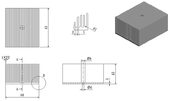
Figure 1.
Thermal resistance measurement apparatus for CPU coolers.
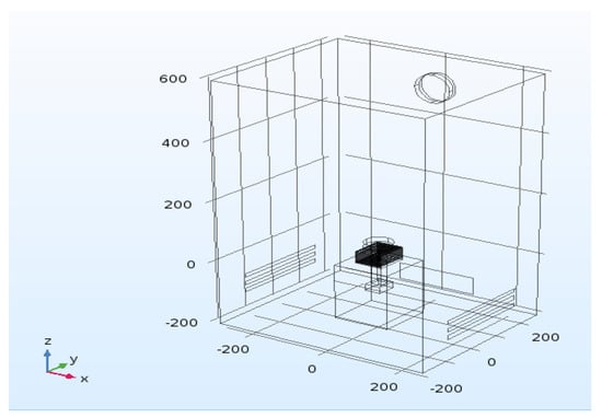
Figure 2.
Model for measuring the thermal resistance of heat dissipation.
A similar device was used to gauge the fins’ thermal resistance. The acrylic materials chamber circulated air, and the base of the heat fin was a square thermal bar with a fixed power source. The other external faces were covered with thermal insulation. The static pressure curve parameters were set for the fan, a fan was positioned near the backplane’s exit, and a fan was installed above the fins. The air entrance, by natural convection, was through the back side panel. A square insulating body was placed in the heat source to cover the area around the heating rod, minimizing heat loss.
In order to reduce the complexity of the problem and the amount of time required for computation, the finite element approach of the software itself was used to calculate heat transfer in this study. The governing equation was described, the heat transfer phenomena in the solution region was calculated, and the basic physical model assumptions were made. The study makes the following assumptions:
- There will be a steady-state heat transfer.
- The fluid in the chamber is three-dimensional forced convection.
- The working fluid has an incompressible density.
- The model space’s walls are all nonslip surfaces.
- There is little radiation impact.
In this numerical analysis, these solvers are step-steady-state and steady-state. The convergence criterion for every iteration of the procedure was specified so that the residual value is below each range. Relative convergence was the criterion in this study. The convergence condition was satisfied when the value falls below 10−4.
3.2. Boundary Conditions
The turbulent flow field is typically used by the numerical simulation flow field. The analysis of the fin heat-dissipation system most frequently uses the k-mode and the k-mode, according to literature. There is not currently a single turbulent flow mode that can handle all issues. Through numerical simulations and experiments, the two groups of models were compared, and in the same construction model, the model that best matched the outcomes of the experiments was chosen. Following an experimental comparison, it was decided to conduct a simulation analysis of the k- turbulent flow model because the results were found to be more accurate. The boundary condition is the setting that matters the most in the numerical simulation. A more complete set of conditions will produce results that are close to the experimental value, but too many conditions will cause the calculation to become overly complex and put the cart before the horse. For this reason, it is crucial to be able to set the proper boundary conditions. Table 1 lists the boundary and physical conditions discussed in this study.

Table 1.
Boundary circumstances Setting.
Physical control and user control were separated in COMSOL software’s mesh design. The latter was employed in this work, and finer mesh configurations were created for various locations, as indicated in Table 2 and Figure 3.
Table 2.
Mesh construction parameters.
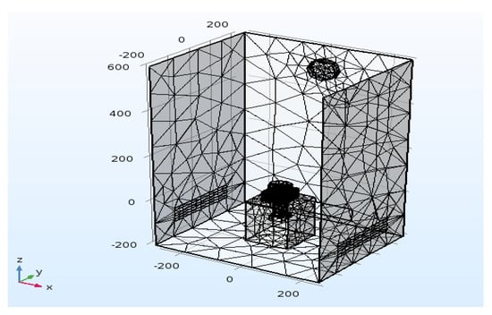
Figure 3.
Mesh of numerical model.
3.3. Experiment Measuring
The data from the thermal imager and anemometer were compared in order to validate the accuracy of the simulation analysis. The basic specifications of the thermal imager (Thermo GEAR G120) were the following:
- (A)
- Measuring range: −40 °C to 500 °C
- (B)
- Resolution: 0.06 °C
- (C)
- Accuracy: ±2 °C or ±2% of reading, whichever was greater
Additionally, the basic specifications of the anemometer (UT-362-USB) were:
- (A)
- Measuring range: 2~30 m/s
- (B)
- Resolution: 0.1 m/s
- (C)
- Accuracy: 2–10 m/s (±3% ± 0.5); 10–30 m/s (±3% ± 0.8)
Figure 4a shows the actual temperature field of the heat sink using an infrared thermal image apparatus and measures the airflow velocity with an anemometer shown in Figure 4b.
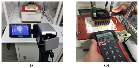
Figure 4.
(a) actual temperature field of the heat sink using an infrared thermal image apparatus; (b) actual airflow velocity using an anemometer.
3.4. Results and Discussion
In order to create models and ideal designs, the response surface method (RSM), an expanded experiment method, combines statistics and optimization techniques. The multiobjective response surface method is the best improvement model. After establishing the design parameters for the heat sink, we used the response surface method’s central composite design to create a factor distribution. The finite element method was then used to analyze the location of the factors. Twenty experiments for the heat sink design were used to provide the results of the simulation study summarized in Table 3 and Figure 5a–c. Based on the above data, we calculated the actual synergistic angle using Equation (9).
Table 3.
Response surface experiment design.
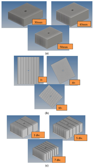
Figure 5.
(a) Fin height, (b) heat sink angle, (c) fin aliquots.
Finding the impact of a particular factor’s magnitude requires regression analysis. As indicated in Table 4 for the field synergy angle and Table 5 for the average fin temperature, if (p < 0.05), the factor could be eliminated and the RSM could be reconstructed.
Table 4.
Experimental regression analysis for the field synergy angle.
Table 5.
Experimental regression analysis for the average fin temperature.
After significance analysis, the expression for the field synergy angle of response surface equation Y1 was as follows:
Y1 = 84.4161 + 0.555736A − 0.113884B − 2.21681C − 0.004475A2 + 0.00100056B2 + 0.2955C2 − 0.00171042A ×
B − 0.0212188A × C + 0.00760208B × C
B − 0.0212188A × C + 0.00760208B × C
Y2 represents the expression for Fin average temperature:
The distribution of the field synergy angle from the bottom to the top of the fin is shown by the XY section in Figure 6a–c. The field synergy angle is approximately 20–50 degrees when viewed from above since the first encounter has a higher flow velocity, but the field synergy angle rises as one approaches the bottom of the fin because the wind speed naturally decreases and the heat transfer enhancement becomes relatively minimal. The opposite has changed with regard to the field synergy angle in the second half of the fin because of the temperature field. The field synergy angle of the fins in the second half is higher because the gradient change and the velocity field change are not coordinated, causing the velocity field change to be unable to keep up with the temperature difference between the fins.
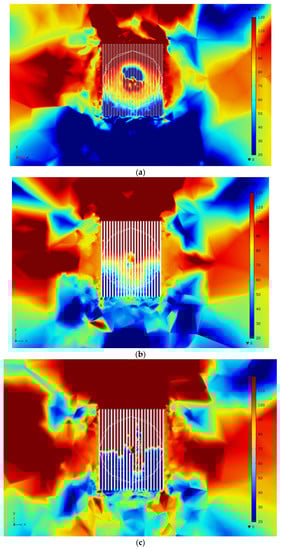
Figure 6.
(a) distribution of the fin’s top field synergy angles; (b) distribution of the fin’s middle field synergy angles; and (c) distribution of the fin’s bottom field synergy angles.
Through a variety of response surface approach experimental designs, the best model was discovered. Table 6 displays the field coangle, velocity, and temperature at the greatest temperature for a single chip. The degree of heat transmission may significantly increase when the fluid enters a jet, and the common interpretation is that as the temperature boundary layer thins, the wall temperature gradient increases. However now, from the standpoint of field synergy, we could look into how wall velocity affects heat transfer. The efficiency of heat dissipation increased with the synchromesh of the display field.
Table 6.
Best optimization combinations.
4. Conclusions
The field synergy idea and multitarget response surface methodology (RSM) were used in a revolutionary heat sink design strategy to maximize the heat transfer. There are some conclusions that can be made:
- We investigated the effects of wall velocity on heat transport due to the field synergy angle. The effectiveness of heat dissipation increased with the synchromesh of the display field.
- The gradient and velocity field changes were not coordinated, which prevented the velocity field change from keeping up with the temperature difference between the fins. This resulted in a higher field synergy angle of the fins in the second half.
- When the synergy angle was employed to show the fins’ effects in heat transfer, the research findings supported the design combination. It is important to show the effectiveness of the heat-dissipation effect.
Author Contributions
Conceptualization, M.-C.L.; methodology, M.-C.L.; software, R.-F.L.; formal analysis, M.-C.L.; investigation, M.-C.L.; data curation, R.-F.L.; writing—original draft preparation, M.-C.L.; supervision, M.-C.L. All authors have read and agreed to the published version of the manuscript.
Funding
This research was funded by the National Kaohsiung University of Science and Technology under Grant No. 111E9010BA02 and the APC was funded by National Kaohsiung University of Science and Technology.
Informed Consent Statement
Not applicable.
Data Availability Statement
Not applicable.
Conflicts of Interest
The authors declare no conflict of interest.
Nomenclature
| cp | Heat capacity, J/(kg∙K) |
| h | Heat transfer coefficient, W/(m2∙K) |
| k | Thermal conductivity, W/(m∙K) |
| l | Length, m |
| Nu | Nusselt number, dimensionless |
| Pr | Prandtl number, dimensionless |
| Q | Conduction heat source, W/m2 |
| Re | Reynold’s number, dimensionless |
| t | Time, s |
| T | Temperature, K |
| U | Fluid velocity field, m/s. |
| Mean velocity vector, m/s. | |
| u | Velocity in the x direction, m/s. |
| v | Velocity in the y direction, m/s. |
| w | Velocity in the z direction, m/s. |
| x | Spatial coordinate |
| Xi | Input factor |
| y | Spatial coordinate |
| yi | Output value |
| Y | Reaction variables |
| z | Spatial coordinate |
| Greek symbols | |
| Velocity boundary layer thickness, m | |
| Temperature boundary layer thickness, m | |
| Fluid density, kg/m3 | |
| μ | Dynamic viscosity, Pa/s |
| ν | Kinematic viscosity, m2/s |
| Field synergistic angle | |
| ▽T | Temperature gradient vector, K |
| ij | Coefficient of the linear and quadratic terms |
References
- Wang, P.; Cui, X.; Weng, J.; Cai, Z.; Cai, R. Experimental investigation of the heat transfer performance of an oscillating heat pipe with LiCl salt solution. Int. J. Heat Mass Transf. 2020, 158, 120033. [Google Scholar] [CrossRef]
- Ji, X.; Yang, X.; Zhang, Y.; Zhang, Y.; Wei, J. Experimental study of ultralow flow resistance fractal microchannel heat sinks for electronics cooling. Int. J. Therm. Sci. 2022, 179, 107723. [Google Scholar] [CrossRef]
- See, Y.; Ho, J.; Leong, K.; Wong, T. Experimental investigation of a topology-optimized phase change heat sink optimized for natural convection. Appl. Energy 2022, 314, 118984. [Google Scholar] [CrossRef]
- Shaeri, M.R.; Sarabi, S.; Randriambololona, A.M.; Shadlo, A. Machine learning-based optimization of air-cooled heat sinks. Therm. Sci. Eng. Prog. 2022, 34, 101398. [Google Scholar] [CrossRef]
- Muneeshwaran, M.; Lee, Y.-J.; Wang, C.-C. Performance improvement of heat sink with vapor chamber base and heat pipe. Appl. Therm. Eng. 2022, 215, 118932. [Google Scholar] [CrossRef]
- Leonardo, M.; Tapas, K.M.; Reddy, K.S. General correlations among geometry, orientation and thermal performance of natural convective micro-finned heat sinks. Int. J. Heat Mass Trans. Sci. Direct. 2015, 91, 711–724. [Google Scholar]
- Bergles, A.E. Heat Transfer Enhancement—The Maturing of Second-Generation Heat Transfer Technology. Heat Transf. Eng. 1997, 18, 47–55. [Google Scholar] [CrossRef]
- Bergles, A.E. Techniques to Enhance Heat Transfer. In Handbook of Heat Transfer, 3rd ed.; Rohsenow, W.M., Hartentt, J.P., Cho, Y.I., Eds.; McGraw-Hill: New York, NY, USA, 1998. [Google Scholar]
- Bergles, A.E. Enhanced Heat Transfer: Endless Frontier, or Maarmature Routine. Enhanced Heat Transfer. 1999, 6, 79–88. [Google Scholar] [CrossRef]
- Guo, Z.Y.; Li, D.Y.; Wang, B.X. A novel concept for convective heat transfer enhancement. Int. J. Heat Mass Transf. 1998, 41, 2221–2225. [Google Scholar] [CrossRef]
- Wang, S.; Li, Z.X.; Guo, Z.Y. Novel concept and device of heat transfer augmentation. In Proceedings of the Eleventh International Conference on Heat Transfer, Kyongju, Korea, 1 November 1998; pp. 405–408. [Google Scholar]
- Li, X.; He, Y.-L.; Tao, W.-Q. Analysis and extension of field synergy principle (FSP) for compressible boundary-layer heat transfer. Int. J. Heat Mass Transf. 2015, 84, 1061–1069. [Google Scholar] [CrossRef]
- Zhao, J.; Huang, S.; Gong, L.; Huang, Z. Numerical study and optimizing on micro square pin-fin heat sink for electronic cooling. Appl. Therm. Eng. 2016, 93, 1347–1359. [Google Scholar] [CrossRef]
- Zhanga, Y.; Liu, X. Application of Field Synergy Principle for Fin Reshaping of a Natural Convection Radiator. In Proceedings of the 9th International Symposium on Heating, Ventilation and Air Conditioning (ISHVAC) and the 3rd International Conference on Building Energy and Environment (COBEE), Tianjin, China, 12–15 July 2015; Volume 121, pp. 1726–1733. [Google Scholar]
- Yao, Y.; Weiwei, W.; Yang, K. Mechanism study on the enhancement of silica gel regeneration by power ultrasound with field synergy principle and mass diffusion theory. J. Heat Mass Transf. 2015, 90, 769–780. [Google Scholar] [CrossRef]
- Hamid, O.A.M.; Zhang, B.; Yang, L. Application of field synergy principle for optimization fluid flow and convective heat transfer in a tube bundle of a pre-heater. Energy 2014, 76, 241–253. [Google Scholar] [CrossRef]
- Ou, J.-J.; Li, L.-F.; Cui, T.; Chen, Z.-M. Application of field synergy principle to analysis of flow field in underhood of LPG bus. Comput. Fluids 2014, 103, 186–192. [Google Scholar] [CrossRef]
- Kundu, B.; Yook, S.J. An accurate approach for thermal analysis of porous longitudinal, spine and radial fins with all nonlinearity effects–analytical and unified assessment. Appl. Math. Comput. 2021, 402, 126124. [Google Scholar] [CrossRef]
- Wankhade, P.A.; Kundu, B.; Das, R. Establishment of non-Fourier heat conduction model for an accurate transient thermal response in wet fins. Int. J. Heat Mass Transf. 2018, 126, 911–923. [Google Scholar] [CrossRef]
- Das, R.; Kundu, B. Forward and Inverse Analyses of Two-Dimensional Eccentric Annular Fins for Space-Restriction Circumstances. J. Thermophys. Heat Transf. 2021, 35, 80–91. [Google Scholar] [CrossRef]
- Kundu, B. Exact Method for Annular Disc Fins with Heat Generation and Nonlinear Heating. J. Thermophys. Heat Transf. 2017, 31, 337–345. [Google Scholar] [CrossRef]
- Liu, C.; Yang, H. Multi-objective optimization of a concrete thermal energy storage system based on response surface methodology. Appl. Therm. Eng. 2021, 202, 117847. [Google Scholar] [CrossRef]
- Mohammed, B.S.; Khed, V.C.; Nuruddin, M.F. Rubbercrete mixture optimization using response surface methodology. J. Clean. Prod. 2018, 171, 1605–1621. [Google Scholar] [CrossRef]
- Mohammed, B.S.; Fang, O.C.; Anwar, H.; Lachemi, M. Mix proportioning of concrete containing paper mill residuals using response surface methodology. Construct. Build. Mater. 2012, 35, 63–68. [Google Scholar] [CrossRef]
- Abdulkadir, I.; Mohammed, B.S.; Liew, M.; Wahab, M. Modelling and multi-objective optimization of the fresh and mechanical properties of self-compacting high volume fly ash ECC (HVFA-ECC) using response surface methodology (RSM). Case Stud. Constr. Mater. 2021, 14, e00525. [Google Scholar] [CrossRef]
- Lin, M.-C.; Lin, R.-F. Innovative design for an active uniform heat dissipation system. Results Phys. 2020, 19, 103355. [Google Scholar] [CrossRef]
Publisher’s Note: MDPI stays neutral with regard to jurisdictional claims in published maps and institutional affiliations. |
© 2022 by the authors. Licensee MDPI, Basel, Switzerland. This article is an open access article distributed under the terms and conditions of the Creative Commons Attribution (CC BY) license (https://creativecommons.org/licenses/by/4.0/).