


Numerical Analysis of Induced Steady Flow on a Bus


Abstract
1. Introduction
2. Materials and Methods
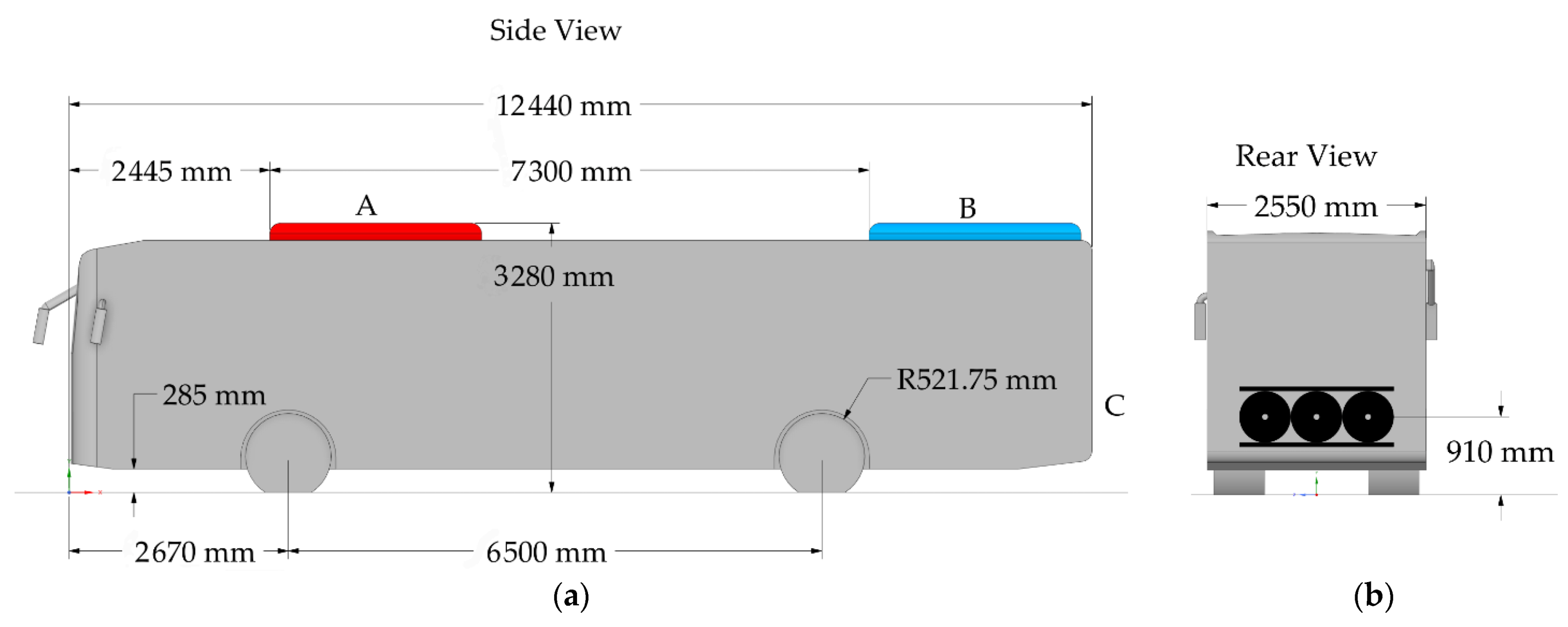
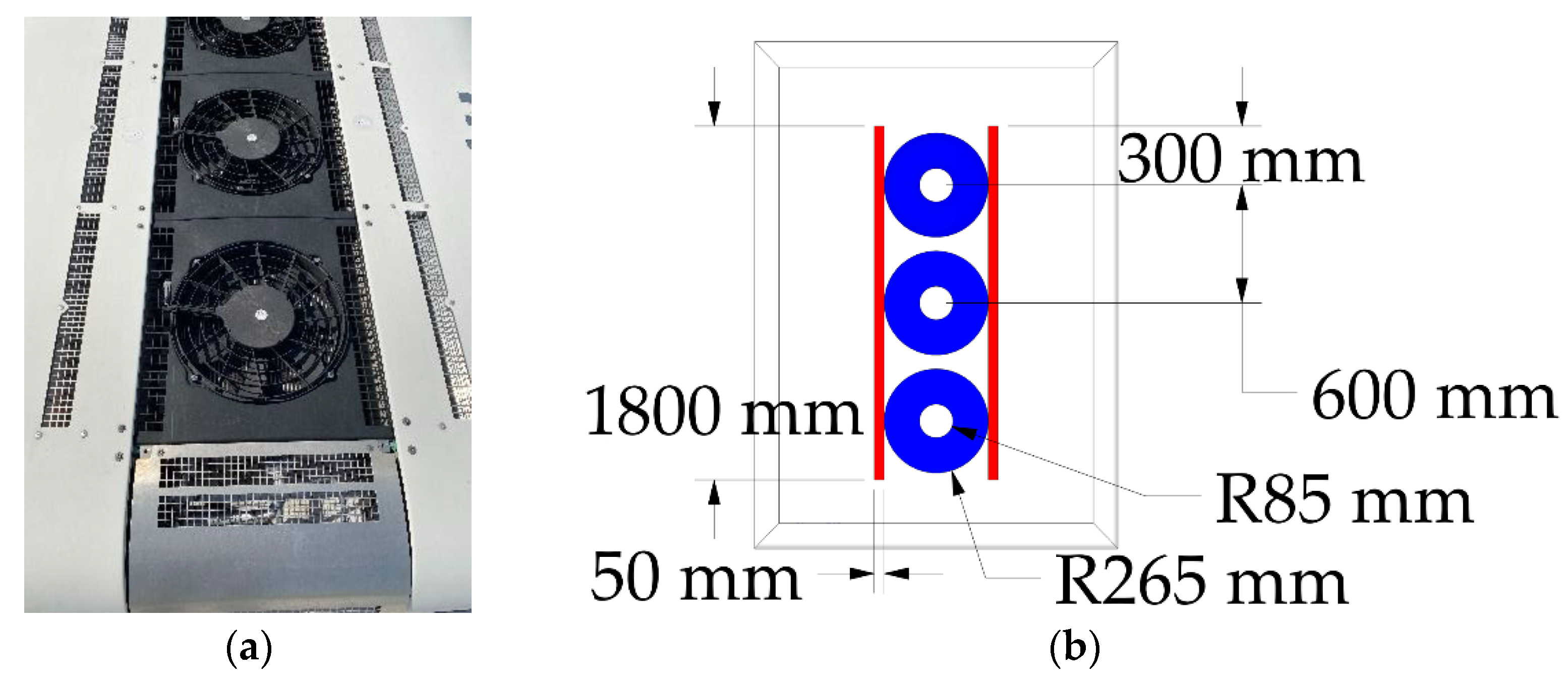
2.1. Geometry
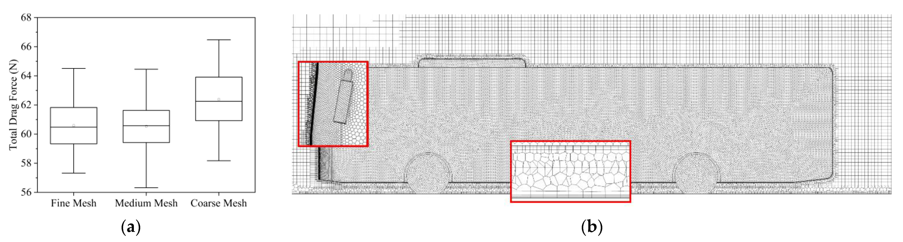
2.2. Mesh
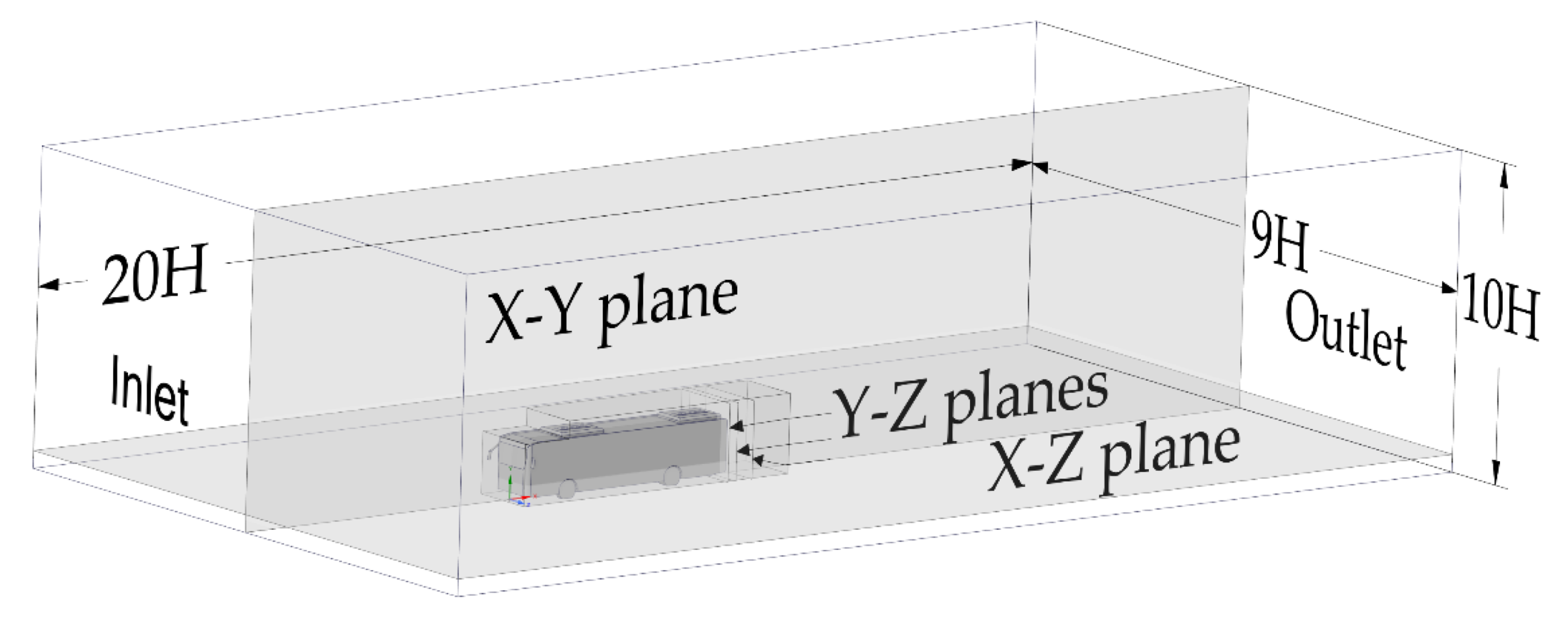
2.3. Numerical Setup
3. Results
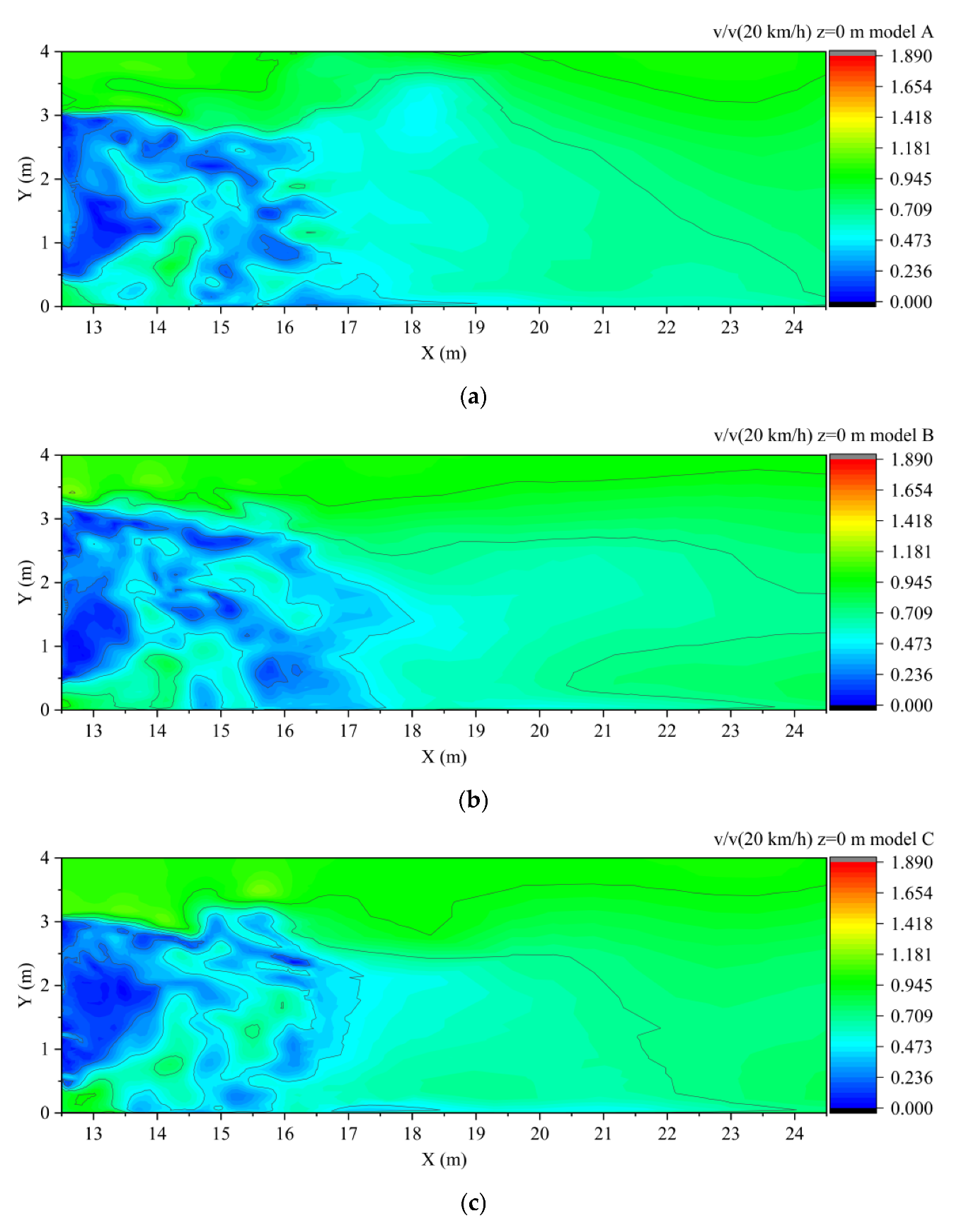
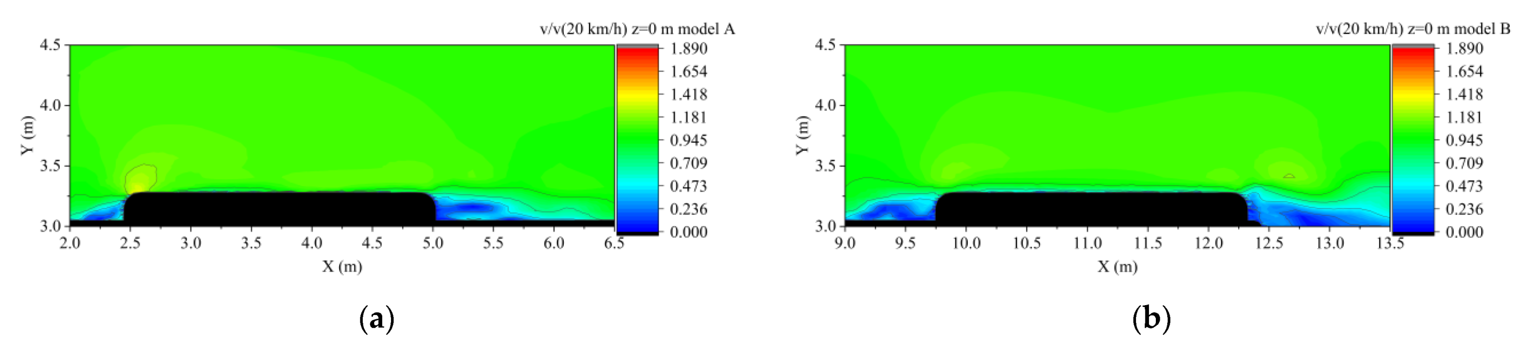
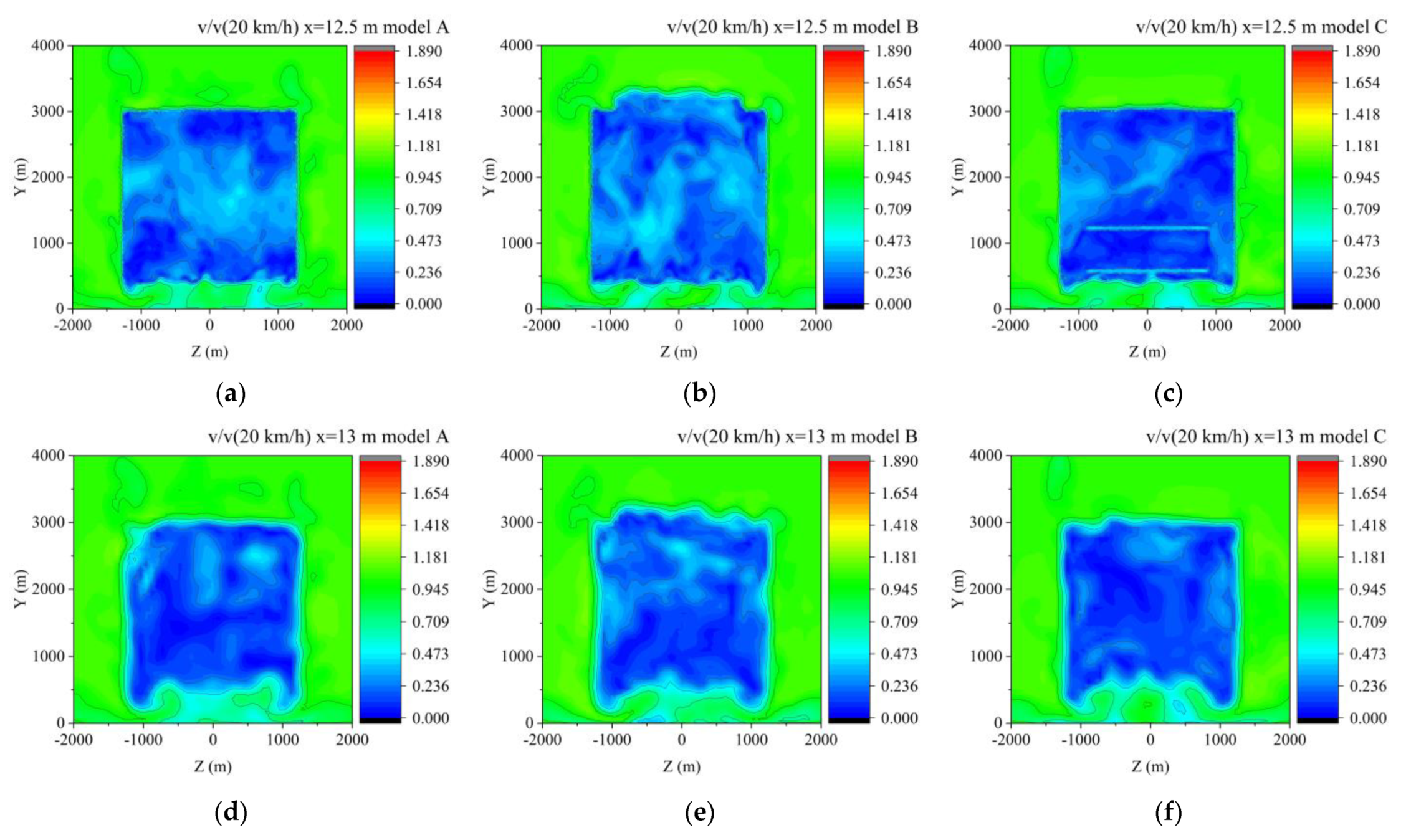
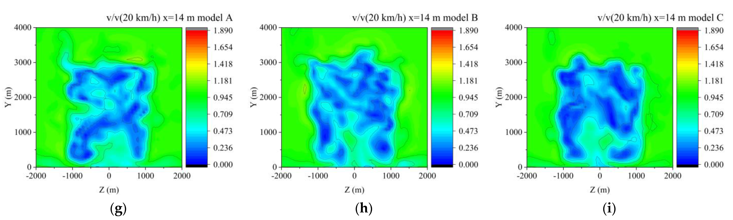
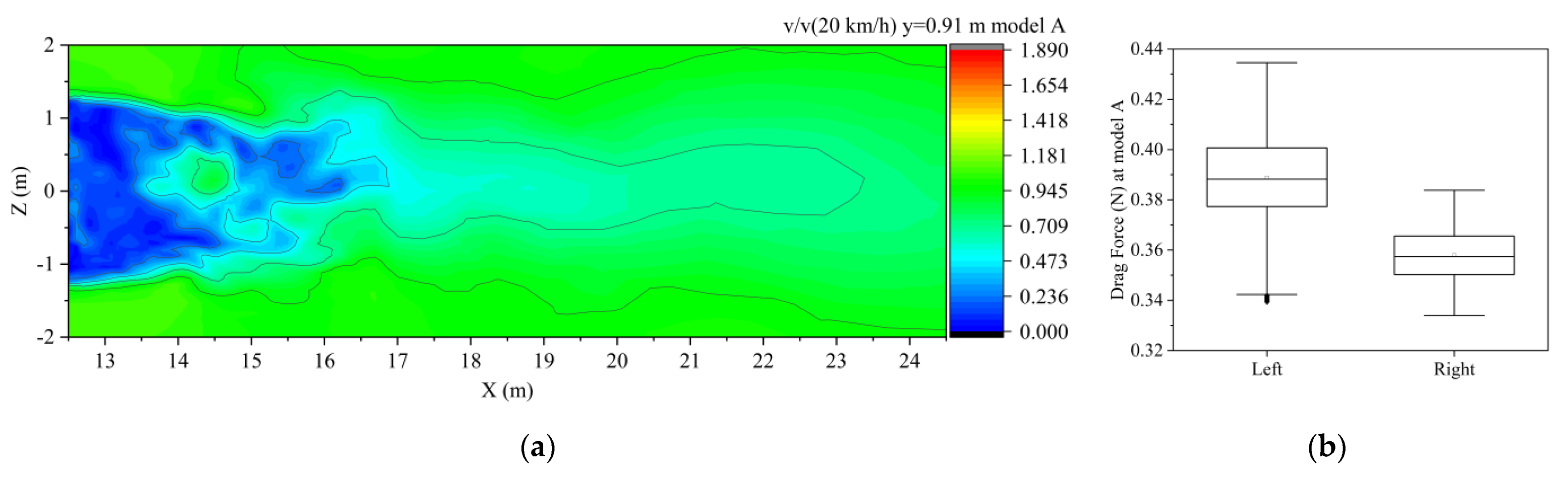
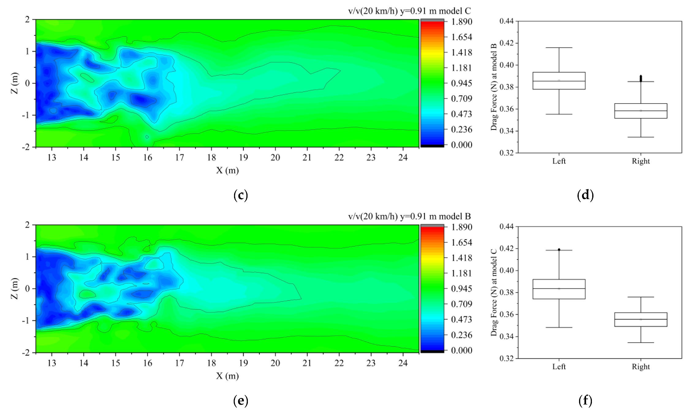
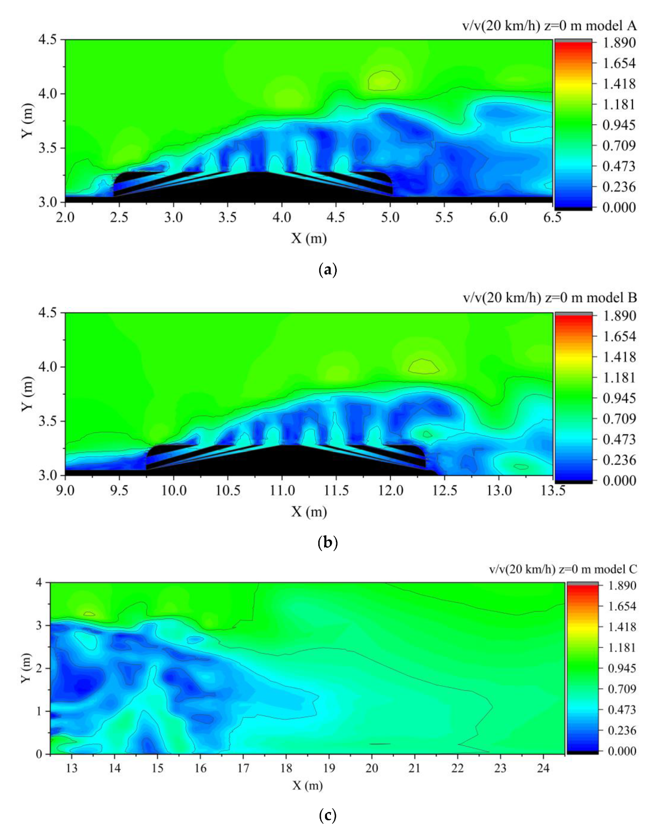
3.1. Velocity Plots
3.2. Induced Flow Patterns
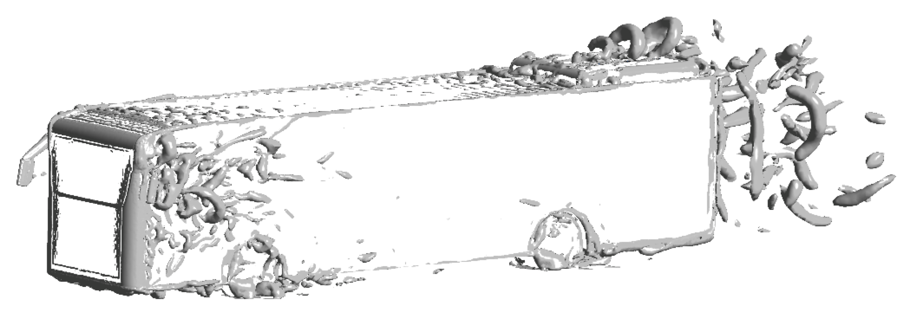
3.3. Q-Criterion
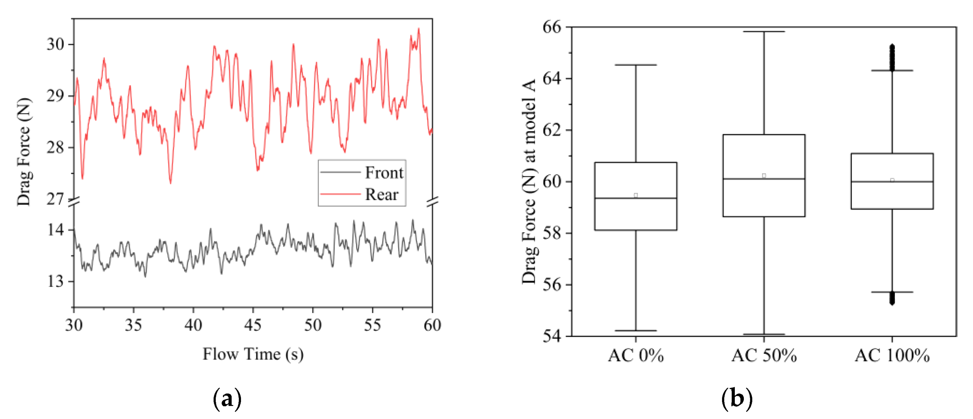
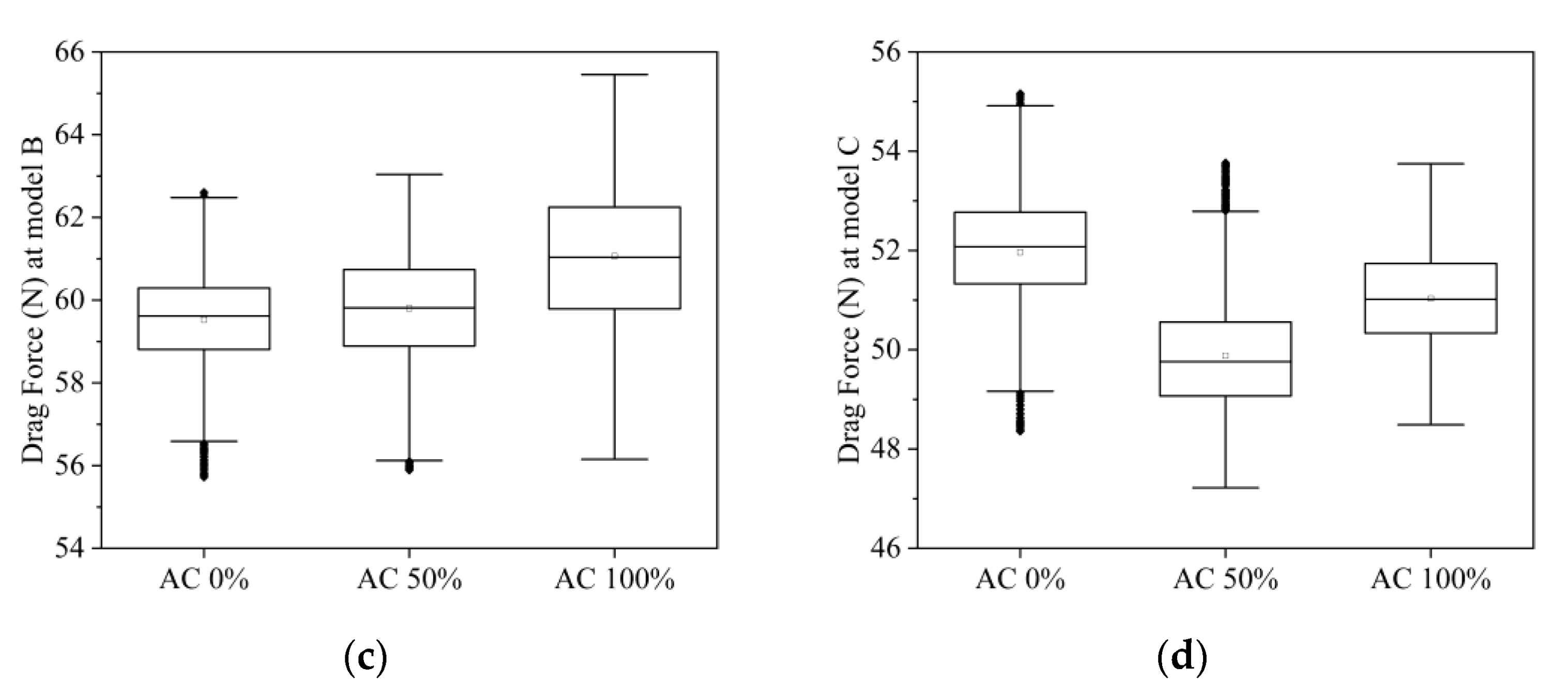
3.4. Force Values
3.5. Drag Coefficients
3.6. Validation
4. Discussion
5. Conclusions
- Flow representation shows that the side-,wind mirror created vortices, but in drag losses, these could be ignored because the difference was within the error range.
- When the fans of the external unit of the air conditioner were activated, O-rings appeared and quickly dissipated.
- The constant flow induced by the external unit of the air conditioner on the roof had a minor increasing effect on drag loss, if it existed at all.
- Drag loss was reduced when the steady flow was induced in the rear of the bus.
- The steady-flow drag-reduction optimum was found to be at 0.26 ReAC/ReW.
- According to the results, placing the box of the external unit in the rear end could result in an 8% drag reduction, meaning a 12.7% energy saving could be realised.
Funding
Data Availability Statement
Acknowledgments
Conflicts of Interest
References
- Bilgili, M.; Aktas, A.E.; Cardak, E. Thermodynamic Analysis of Bus Air Conditioner Working with Refrigerant R600a. Eur. Mech. Sci. 2017, 1, 69–75. [Google Scholar] [CrossRef]
- Sylla, F.K.; Faye, A.; Diaw, M.; Fall, M.; Tal-Dia, A. Traffic Air Pollution and Respiratory Health: A Cross-Sectional Study among Bus Drivers in Dakar (Senegal). Open J. Epidemiol. 2018, 8, 81699. [Google Scholar] [CrossRef]
- Shen, Y.; Li, C.; Dong, H.; Wang, Z.; Martinez, L.; Sun, Z.; Handel, A.; Chen, Z.; Chen, E.; Ebell, M.H.; et al. Community Outbreak Investigation of SARS-CoV-2 Transmission among Bus Riders in Eastern China. JAMA Intern. Med. 2020, 180, 1665–1671. [Google Scholar] [CrossRef]
- Zhang, Z.; Han, T.; Yoo, K.H.; Capecelatro, J.; Boehman, A.L.; Maki, K. Disease transmission through expiratory aerosols on an urban bus. Phys. Fluids 2021, 33, 015116. [Google Scholar] [CrossRef] [PubMed]
- Gilliéron, P.; Kourta, A. Aerodynamic drag control by pulsed jets on simplified car geometry. Exp. Fluids 2013, 54, 1457. [Google Scholar] [CrossRef]
- Tounsi, N.; Mestiri, R.; Keirsbulck, L.; Oualli, H.; Hanchi, S.; Aloui, F.; Algiers, E.M.P.O.; Leste, N.D.D.M. Experimental study of flow control on bluff body using piezoelectric actuators. J. Appl. Fluid Mech. 2016, 9, 827–838. [Google Scholar] [CrossRef]
- Szodrai, F. Quantitative Analysis of Drag Reduction Methods for Blunt Shaped Automobiles. Appl. Sci. 2020, 10, 4313. [Google Scholar] [CrossRef]
- Bayındırlı, C. Drag reduction of a bus model by passive flow canal. Int. J. Energy Appl. Technol. 2019, 6, 24–30. [Google Scholar] [CrossRef]
- Pastoor, M.; Henning, L.; Noack, B.R.; King, R.; Tadmor, G. Feedback Shear Layer Control for Bluff Body Drag Reduction. J. Fluid Mech. 2008, 608, 161–196. [Google Scholar] [CrossRef]
- Aubrun, S.; McNally, J.; Alvi, F.; Kourta, A. Separation flow control on a generic ground vehicle using steady microjet arrays. Exp. Fluids 2011, 51, 1177–1187. [Google Scholar] [CrossRef]
- Littlewood, R.P.; Passmore, M.A. Aerodynamic drag reduction of a simplified squareback vehicle using steady blowing. Exp. Fluids 2012, 53, 519–529. [Google Scholar] [CrossRef]
- Szodrai, F. Numerical Assessment of Side-Wind Effects on a Bus in Urban Conditions. Appl. Sci. 2022, 12, 5688. [Google Scholar] [CrossRef]
- Hamit, S.; Yakup, İ. Drag Coefficient Determination of a Bus Model Using Reynolds Number Independence. Int. J. Automot. Eng. Technol. 2015, 4, 146–151. [Google Scholar]
- Muthuvel, A.; Murthi, M.K.; Sachin, N.P.; Koshy, V.M.; Sakthi, S.; Selvakumar, E. Aerodynamic Exterior Body Design of Bus. Int. J. Sci. Eng. Res. 2013, 4, 2453–2457. [Google Scholar]
- Roache, P.J. Perspective: A method for uniform reporting of grid refinement studies. ASCE J. Fluids Eng. 1994, 116, 405–413. [Google Scholar] [CrossRef]
- Nicoud, F.; Ducros, F. Subgrid-scale stress modelling based on the square of the velocity. Flow Turbul. Combust. 1999, 62, 183–200. [Google Scholar] [CrossRef]
- Vámosi, A.; Czégé, L.; Kocsis, I. Development of Bus Driving Cycle for Debrecen on the Basis of Real-traffic Data. Period. Polytech. Transp. Eng. 2022, 50, 184–190. [Google Scholar] [CrossRef]
- Lajos, T.; Preszler, L.; Finta, L. Effect of moving ground simulation on the flow past bus models. J. Wind Eng. Ind. Aerodyn. 1986, 22, 271–277. [Google Scholar] [CrossRef]
- Gurlek, C.; Sahin, B.; Ozkan, G.M. PIV studies around a bus model. Exp. Therm. Fluid Sci. 2012, 38, 115–126. [Google Scholar] [CrossRef]
- Hunt, J.C.R.; Wray, P.M.A.A. Eddies, Stream, and Convergence Zones in Turbulent Flows. In Center for Turbulence Research, Proceedings of the Summer Program; 1988; pp. 193–208. Available online: https://web.stanford.edu/group/ctr/Summer/201306111537.pdf (accessed on 28 October 2022).
- Krajnović, S.; Davidson, L. Numerical study of the flow around a bus-shaped body. J. Fluids Eng. Trans. ASME 2003, 125, 500–509. [Google Scholar] [CrossRef]
- Zhu, J.J.; Liu, G.W. Numerical optimization for aerodynamic noises of rear view mirrors of vehicles based on rectangular cavity structures. J. Vibroeng. 2018, 20, 1240–1256. [Google Scholar] [CrossRef]
- Chu, Y.J.; Shin, Y.S.; Lee, S.Y. Aerodynamic analysis and noise-reducing design of an outside rear view mirror. Appl. Sci. 2018, 8, 519. [Google Scholar] [CrossRef]
- Chode, K.K.; Viswanathan, H.; Chow, K. Noise emitted from a generic side-view mirror with different aspect ratios and inclinations. Phys. Fluids 2021, 33, 084105. [Google Scholar] [CrossRef]
- Janna, W.S.; Schmidt, D. Fluid Mechanics Laboratory Experiment: Measurement of Drag on Model Vehicles. In Proceedings of the ASEE Southeast Section Conference, 2014. Available online: http://se.asee.org/proceedings/ASEE2014/Papers2014/4/11.pdf (accessed on 28 October 2022).
- Jadhav, C.R.; Chorage, R.P. Modification in commercial bus model to overcome aerodynamic drag effect by using CFD analysis. Results Eng. 2020, 6, 100091. [Google Scholar] [CrossRef]


| Cases | yH fine | yH | Δmin | Δmax fine | Δmax | Cell Count |
|---|---|---|---|---|---|---|
| Fine Mesh | 0.1 mm | 1 mm | 20 | 40 mm | 320 mm | 8.6 × 10⁶ |
| Medium Mesh | 0.2 mm | 2 mm | 40 | 80 mm | 640 mm | 1.8 × 10⁶ |
| Coarse Mesh | 0.4 mm | 4 mm | 80 | 160 mm | 1280 mm | 0.4 × 10⁶ |
| Cases | Average Orthogonal | Average Skewness | Average Aspect Ratio | GCI |
|---|---|---|---|---|
| Fine Mesh | 0.97 | 0.03 | 4.6 | 0.007% |
| Medium Mesh | 0.96 | 0.04 | 5.3 | - |
| Coarse Mesh | 0.95 | 0.05 | 5.7 | 0.254% |
| Type | Magnitude | Comment |
|---|---|---|
| Inlet | 20 km∙h−1 | Velocity inlet |
| Ground | 20 km∙h−1 | No-slip moving wall |
| Tyre surface | 20 km∙h−1 | No-slip moving wall |
| Rim | 20 km∙h−1/radius | No-slip rotating wall |
| Outlet | 1 atm total pressure | Pressure outlet |
| AC | 6960 m3∙h−1 | Mass flow inlet and outlet (ρ = 1.225 kg∙m−3) |
| Bus | - | No-slip stationary wall |
| Walls of the wind tunnel | - | Symmetry condition |
| Drag Coefficients | Model A | Model B | Model C |
|---|---|---|---|
| AC 0% flow rate | 0.395 ± 0.007 (base) | 0.394 ± 0.013 (0%) | 0.363 ± 0.008 (−8%) |
| AC 50% flow rate | 0.396 ± 0.008 (0%) | 0.399 ± 0.014 (1%) | 0.348 ± 0.008 (−12%) |
| AC 100% flow rate | 0.405 ± 0.011 (+3%) | 0.398 ± 0.012 (1%) | 0.356 ± 0.007 (−10%) |
| Drag Coefficient | Comment | Source |
|---|---|---|
| 0.395 ± 0.007 | 20 km∙h−1 with mirrors | Current study |
| 0.389 ± 0.010 | 20 km∙h−1 without mirrors | Previous study [12] |
| 0.65 | 36 km∙h−1 | Cihan Bayındırlı [8] |
| 0.43 | 80 km∙h−1 | Muthuvel et al. [14] |
| 0.66 | 100 km∙h−1 | Hamit et al. [13] |
| 0.65 | 120 km∙h−1 | Jadhav et al. [26] |
| 0.41 | modified | Jadhav et al. [26] |
| Relative Energy Saving | Model A | Model B | Model C |
|---|---|---|---|
| AC 0% flow rate | baseline | 0.1% | 12.7% |
| AC 50% flow rate | −0.5% | −1.2% | 16.2% |
| AC 100% flow rate | −2.6% | −0.9% | 14.3% |
Publisher’s Note: MDPI stays neutral with regard to jurisdictional claims in published maps and institutional affiliations. |
© 2022 by the author. Licensee MDPI, Basel, Switzerland. This article is an open access article distributed under the terms and conditions of the Creative Commons Attribution (CC BY) license (https://creativecommons.org/licenses/by/4.0/).
Share and Cite
Szodrai, F. Numerical Analysis of Induced Steady Flow on a Bus. Energies 2022, 15, 8444. https://doi.org/10.3390/en15228444
Szodrai F. Numerical Analysis of Induced Steady Flow on a Bus. Energies. 2022; 15(22):8444. https://doi.org/10.3390/en15228444
Chicago/Turabian StyleSzodrai, Ferenc. 2022. "Numerical Analysis of Induced Steady Flow on a Bus" Energies 15, no. 22: 8444. https://doi.org/10.3390/en15228444
APA StyleSzodrai, F. (2022). Numerical Analysis of Induced Steady Flow on a Bus. Energies, 15(22), 8444. https://doi.org/10.3390/en15228444