Energy Analysis and Cost-Effective Design Solutions for a Dual-Source Heat Pump System in Representative Climates in Europe

Abstract

Ground-source heat pumps are an efficient technology for heating and cooling in buildings. However, the main limitation of their widespread application is the borehole heat exchanger’s (BHE) high investment cost. Hybridizing GSHP systems may overcome this limitation. This research work analyzes the long-term energy performance of a dual-source heat pump (DSHP) system, which uses the air or the ground as external heat/sink sources, in three representative European climates. First, a BHE cost-effective design solution is proposed for each climatology; then, a complete energy analysis is carried out, and the optimal source control parameters that best enhance the system performance in each climate are determined with the use of a complete dynamic model of the DSHP system developed in TRNSYS. Simulations were carried out for a 25-year operation period. Results show that the DSHP maintains the efficiency during the simulated period, with deviations lower than 1.7% in all cases. Finally, the source control optimization method results in only slight efficiency gains (<0.35%) but with a stronger effect on the ground/air use ratio (up to 25% use of air in cold climates), reducing the thermal imbalance of the ground and leading to a consequent BHE size length and cost reduction.

1. Introduction

Currently, shallow geothermal applications commonly known as ground-source heat pump (GSHP) systems are the most widespread geothermal heat pump technology in Europe [1]. According to a European Geothermal Energy Council (EGEC) report, in 2014, the European shallow geothermal market was estimated by the capacity of at least 19,000 MW_th distributed over about 1.4 million GSHP installations [2]. Just a few years later, in 2019, the EGEC reported that Europe reached the milestone of two million geothermal heat pumps installed, becoming a mainstream heating and cooling solution in some regional and national markets, primarily in countries with colder climates such as Sweden, where a record number of 13 GSHPs accounts for 100 households on average [3]. The main advantage of shallow GSHP systems is their high flexibility. They can be installed and used anywhere, regardless of geographical location or ground conditions, may be combined with many heat sources, and work in a reversible cycle, providing heat both in the summer and winter season. This is why, in the past 20 years in the EU, the number of shallow geothermal systems is gradually growing at an average rate of 3% and now can be found everywhere across Europe [1]. Nevertheless, it is the north and central European countries that account for most of the installed potential. In 2016, Sweden along with Germany, France, and Switzerland had the highest number of GSHP systems among all European countries, corresponding to 69% of the total installed capacity [2].

Often, to compare the feasibility of the GSHPs with other HVAC systems, the conventional air-source heat pump (ASHP) is used as a reference [4,5,6]. Due to the variation in external air temperature throughout the year, ASHPs are characterized by a variable energy performance which often leads to lower overall system efficiency, especially in cold climates. On the other hand, GSHPs take advantage of a more stable external heat source and thus significantly enhance the heat pump’s efficiency. Despite that, their application is not as widespread as the ASHPs, mainly due to the high cost of the ground-source heat exchanger (GSHE). A GSHE, installed vertically or horizontally to exchange the heat with the soil, is the main component of a GSHP. Although the most energy-efficient GSHP configuration is achieved by coupling it with a vertical borehole heat exchanger (BHE), the main drawback of BHE systems is their high investment cost compared to horizontal configurations. Avoiding the over-sizing of the BHE leads to a lower investment cost; therefore, an accurate assessment of thermal loads is necessary. For this purpose, many types of simulation software are used, such as GLHEPro [7], EED [8], or TRNSYS [9]. According to the European Technology and Innovation Platform on Renewable Heating & Cooling (RHCETIP), one of the key actions in the research and innovation on shallow geothermal energy foreseen in the new Horizon Europe program will be enhancing the use of simulation tools for optimization of the performance of geothermal systems by the integration of subsurface models into the building energy models, which may lead to a reduction in the length of the vertical heat exchanger. The detailed objectives, performance indicators, and the implementation timeline for the specified key actions can be found in the RHCETIP’s 2020 report [1].

The further reduction in the borehole length might be obtained by hybridizing the GSHP with an additional heat source, for instance, the air. In such a way, the hybrid heat pump alternates between the air and the ground as external heat sources, potentially overcoming some of the limitations of the two most common ASHP and GSHP systems. For example, Grossi et al. concluded that a dual-source heat pump (DSHP) that chooses between the air or the ground as an external heat source can work with up to 50% shorter BHE fields [10]. Another recent study by Marinelli et al. compares the environmental impact of a DSHP air/ground system with conventional solutions, concluding that in humid climates, the dual-source technology is more environmentally friendly than ASHP. Moreover, in comparison with GSHP, using shorter geothermal probes for the BHE once again leads to a reduction in the environmental impact [11]. In terms of using the heat as an additional energy source for a hybrid GSHP system, another dual-thermal configuration was studied by Rayegan et al. where a BHE is coupled with a solar-assisted desiccant cooling system and assessed in hot and humid climates [12]. In this configuration, the solar evacuated tube collectors are used to generate additional heat to store up any deficit from the geothermal heat pump. Both ground and solar systems are used for regenerating the desiccant wheel and a pre-cooling process, respectively. The authors conclude that in the simulations with the absence of the GSHE, the system cannot provide thermal comfort in extremely humid regions, even with high regeneration temperatures; meanwhile, for simulations with the BHE, the established thermal comfort improves significantly.

Apart from coupling the GSHP system with a different external heat source, a hybrid configuration can also be achieved by using a supplementary electricity source, for example, solar photovoltaic energy. This configuration is particularly interesting from an economical perspective because the electricity necessary for running the compressor of the heat pump is supplied by means of the PV modules. Such a system is described in research work by Kavian et al., where three different module types with polycrystalline, monocrystalline, and thin-film cells are analyzed in order to determine the best system performance from the irreversibility and economic points of view [13]. Moreover, in this study, a single GSHP is compared with a hybrid PV/GSHP system; apart from reaching lower values of the levelized cost of electricity (LCOE), in the case of a DSHP, the hybrid system has a lower carbon footprint of around 30%. Another example of using solar energy for the hybrid GSHP system is the photovoltaic/thermal (PVT) module, which allows using waste thermal energy from photovoltaic panels as an inlet water source for the ground-source heat pump system. Recent studies show that in this configuration, not only can the otherwise lost heat be partially recovered, but it can also be used to cool the PV module and increase its electrical efficiency [14,15]. Moreover, similarly to the PV/GSHP hybrid system, the authors anticipate many economic benefits, such as a short discounted payback (DPB) period (5–6 years), for the most optimal configurations. A recent review of the solar-assisted heat pumps, including GSHPs, ASHPs, and others, can be found in the following reference [16]. Additionally, another review of hybrid heat pumps presents a higher variety of possibilities for the integration of the GSHP, such as cooling towers, gas boilers, biomass reactors, electric heaters, and chillers [17].

Many different factors influence the performance of the BHE in a GSHP system. A commonly known parameter for describing the efficiency of a heat pump is the coefficient of performance (COP), which in the case of heating mode can be described as the relation between the heat transfer in the condenser (or evaporator in the case of cooling mode) and the total input power consumed by the device [18] and usually varies linearly with the carrying fluid outlet temperature [19]. A work by Tang et al. investigates the influence of 15 different factors (meteorological condition, hydraulic condition, the grout thermal conductivity, carrying fluid material, etc.) on the yearly average heat pump COP for the shallow BHE. The study concludes that the factor with the highest impact on the BHE performance is the meteorological condition (defined by three different climate conditions) where the measured COP values had up to 45.3% of difference [20]. The result of this study indicates the importance of energy assessment and optimization of GSHP systems in different climate conditions. Moreover, the economic feasibility of the GSHP systems in different climates is also often a subject of research. For example, a work by Rivoire et al. compares the feasibility of GSHP and hybrid GSHP/gas boiler systems installed in different building types and under different climate conditions. The economic analysis results reveal that public subsidies are essential to ensure the profitability of investment, as far as the European energy prices are concerned [21]. Another result for the simulations with a single GSHP system is that, in case of the absence of subsidies, the only climate zone that reached the “feasible” or “almost feasible” status for every building type (house, office, and hotel) was the zone with moderate climate conditions (Madrid, Bologna, Thessaloniki). For such conditions, a balance between the heating and cooling operating hours is maintained, which is favorable in the case of reversible heat pumps because it reduces the thermal imbalance of the ground and hence the required length of the borehole. The authors conclude that from an economic perspective, in colder climates, it is more beneficial to hybridize the GSHP with a conventional heat source, although it is achieved at the expense of slightly lower CO₂ reduction [21].

One of the possible solutions to overcome the mentioned constraints is to couple the GSHP with a reverse-cycle air conditioner. Recent work by Aditya et al., in which an exemplary building is simulated in ten different cities, compares the economic feasibility of such a hybrid air/ground heat pump with four other conventional systems. As a result, in 7 out of 10 analyzed cities, the DSHP is considered the most cost-efficient solution [22]. Although the results of the study cover a significant number of climatic conditions as well as potential changes in key parameters, the analysis does not consider a wider range of building types and characteristics, and more importantly, the DSHP is not optimized nor properly modeled as an independent system component.

However, such an example of a novel air/ground-source DSHP unit, installed in three demonstration facilities in Europe, can be found in the GEOTeCH project, co-funded by the European Commission as a part of the H2020 program [23]. Experimental real operation data from one of the demo sites can be found in the work by Zanetti et al. [24], where the authors have used this data to validate a model of the heat pump. In the framework of this four-year project, several studies were developed. A novel “plug-and-play” DSHP, capable of working in eleven operating modes, was designed and modeled in TRNSYS, which is described by Corberán et al. in the following study [25]. Another work, by Cazorla-Marín et al., in which the integrated DSHP system was adapted to three different locations in Spain (Valencia, Madrid, Bilbao), analyzed the percentage of operation of the DSHP under each of the selected working modes [26]. An extension to this study, where an office building with the DSHP unit is simulated for three different European cities with representative climates—Strasbourg (average climate), Athens (warmer climate), and Stockholm (colder climate)—concluded that in warmer climates the use of DSHP is not as profitable as in cold climates, as the air is used to satisfy only 4% of the thermal energy demand [27]. Another work by Cazorla-Marín et al. consisted of the implementation of a coaxial borehole heat exchanger TRNSYS type into the previously developed DSHP model, which allowed for both short- and mid-term simulations [28]. The most recent study regarding this DSHP pump unit, where different optimization strategies were tested using data from the demo site in Amsterdam, was presented at the 8th Iberian-American Congress of Refrigeration Science and Technology [29].

This research work complements the studies developed in GEOTeCH’s framework. While the energy performance of the modeled DSHP is analyzed in detail in the previously mentioned publications [26,27], both studies assumed the same BHE size for all analyzed locations. In addition, the long-term energy assessment was excluded from the analysis, as the system performance was examined in only one year of operation. Additionally, the energy assessment conducted in the latest work [29], in which various strategies for the DSHP system optimization are analyzed, is focused on only one climatic condition. Moreover, while in the previously described study [22] the DSHP system performance is analyzed under different climatic conditions, the simulated exemplary building has the same insulation parameters for each climate, and the unique constructive typology was not considered for each location specified in the study. The study attributes its novelty to an individual approach for the evaluation of the energy performance of the DSHP system in three European representative climate types (warm, average, and cold), including the individual design of the main component of the system, the spiral coaxial BHE. In addition, the energy assessment performed in the study takes a long-term approach, as the DSHP operation is examined in 25 years. Finally, the optimization strategies are adapted to the source control of the DSHP system to find the best solution for each representative climatology.

2. Methodology

2.1. TRNSYS Model

The tool used for simulating the dynamic energy performance of the system is the DSHP model developed in TRNSYS. The model was designed in the framework of the GEOTeCH project and, in the past years, was gradually enhanced by additional system components, such as the coaxial spiral BHE, and is described in numerous scientific publications [25,26,27,28,30]. The system designed in TRNSYS is modular, and its key elements that describe different components are grouped in macros mutually interconnected and governed by mathematical relations. 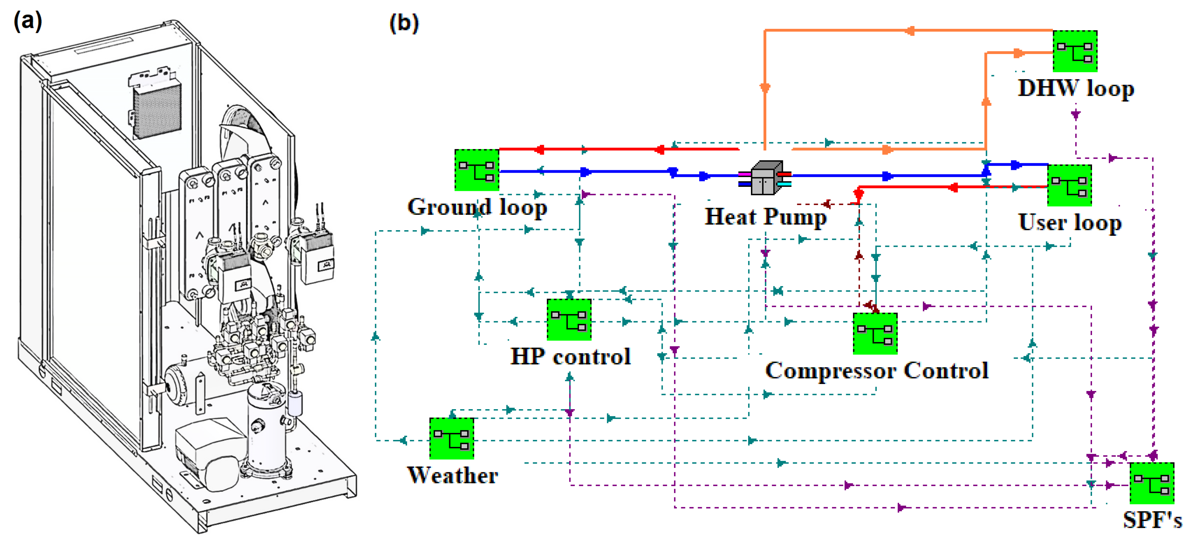Figure 1b) represents the arrangement of macros within the model where the key elements are two control systems (PID and differential controllers), three different hydraulic loops (user loop, DHW loop, and the ground loop), system efficiency, and weather data. The core element in the system model is the heat pump, where the water coming from the different circuits is heated up or cooled down depending on the system control and the thermal demand. The final version of the model is extensively described in the Ph.D. dissertation by Cazorla-Marín [30] and includes in-depth specifications of all control strategies and subsystems.

2.1.1. Heat Pump Model

The type “HP-Geotech_v3” corresponds to the DSHP model, based on the DSHP prototype developed in the GEOTeCH project, which is able to produce heating or cooling to the user, as well as to produce DHW using the air as a source/sink or the ground loop. This model was developed in previous works [25,30] and is defined as a black box in the TRNSYS model. The DSHP performance is calculated using polynomial correlations obtained from a test campaign [31] and calculated with the software IMST-ART [32]. These correlations calculate the evaporator and condenser capacities and the compressor power, as a function of the working mode and the different operating conditions: inlet temperature in evaporator and condenser, temperature difference in the evaporator and condenser, compressor frequency, air temperature, and fan speed.

2.1.2. Ground Loop

In the ground loop, the spiral coaxial BHE field is defined, including the piping. An average coaxial BHE is modeled and coupled with a long-term ground model. The BHE model used (B2G model) was developed by Cazorla-Marín et al. to reproduce the dynamic behavior of a coaxial BHE [28]. Additionally, the long-term response of the ground, as well as the interaction between the different BHEs in the field, is considered in the ground loop using a model based on the infinite line source (ILS) model, called “Line Source Approach” (LSA) model and described in [30]. The ground loop macro is shown in Figure 2.

2.1.3. DHW Loop

The DHW loop includes an insulated storage tank with internal coil heat exchanger, the control for the DHW production, mixing valves, and the DHW demand. The DHW demand profile is based on the profile in the ASHRAE Handbook—HVAC Applications [33], and it is introduced as an external file. The DHW macro is shown in Figure 3.

2.1.4. User Loop

The user loop includes a buffer tank in the supply side, a circulation pump (with CP control system), piping, and the user demand. The building model is not included in the DSHP model. However, the thermal demand of the building, defined as hourly thermal loads, is introduced as an input to perform the simulations. This thermal demand was previously calculated with a building model, depending on the weather conditions, as explained in Section 2.2. This macro is shown in Figure 4.

2.1.5. Compressor Control

In this macro, the frequency of the variable speed compressor is defined in order to adapt the capacity of the heat pump to the instantaneous thermal demand based on the supply temperature in the user circuit. For this purpose, a PID controller (type 23) is used with only proportional and integral actions. This PID compares the supply temperature to the set point and varies the compressor frequency to reach the set point value. In addition, a differential controller with hysteresis (type 2b) is used to control the cycling of the compressor at the minimum frequency (when the thermal demand is very low). The minimum and maximum frequency of the compressor can be set as parameters in the model.

2.1.6. Weather

The weather conditions are defined by introducing an input weather file that corresponds to a given location. The ambient temperature at each time step is used as the air temperature in the DSHP model but also for the calculation of thermal losses in pipes and tanks, as well as to select the most favorable source.

2.1.7. SPFs

In this macro, the consumption of the different components is considered to calculate the system consumption as well as its efficiency. In order to analyze the system efficiency, seasonal performance factors (SPFs) are defined, as defined in Section 2.5. The consumption of the heat pump compressor and parasitic losses is calculated in the heat pump type, but the circulation pumps’ consumption is calculated in this macro based on experimental correlations, as a function of the flow rate and pressure drop in each circuit.

2.1.8. HP Control

This is the macro where the main operation parameters are set: working schedule (DHW production and air-conditioning operation), thermal source control (selection of the most favorable source/sink, depending on the air and ground temperatures, as described in Section 2.6), and operating mode selection. The DSHP is able to work in 11 different operating modes, which are defined in

Table 1. DSHP system operating modes.

Season	Condenser	Evaporator	Operating Mode
Summer	Air	User	M1-Summer Air
	Ground	User	M2-Summer Ground
	-	-	M10-Free cooling
	DHW	User	M3-DHW User “Full Recovery”
	DHW	Air	M6-DHW Air
	DHW	Ground	M8-DHW Ground
	DHW	Air	M11-Freecooling + DHW Air
Winter	User	Air	M4-Winter Air
	User	Ground	M5-Winter Ground
	DHW	Air	M7-DHW Air
	DHW	Ground	M9-DHW Ground

.

Depending on the season (summer or winter), the air conditioning will provide cooling or heating, respectively. In parallel, the heat pump can provide DHW. In addition, the DSHP alternates between ground and air as a source or sink, totaling 8 modes. The ninth operation mode (labeled as “M3-DHW User Full recovery”) allows the simultaneous production of cooling and DHW, coupling the evaporator to the user circuit and the condenser to the DHW production.

Two additional free-cooling modes are defined for summer operation: M10 and M11. When the outlet borehole temperature is cold enough to cover the cooling demand, M10 is selected. Using this method, the thermal fluid bypasses the heat pump, sending the cold water to a heat exchanger, where it directly cools down the user circuit water. Finally, M11 offers simultaneous free cooling and DHW production.

2.2. Building Typology and Thermal Demand

The building and its corresponding thermal demand analyzed in the study were previously modeled by Ruiz-Calvo et al. [34]. The building belongs to the Department of Applied Thermodynamics situated on the campus of the Polytechnic University of Valencia, Spain. The building was constructed in the 1970s, and in the past, its thermal demand was partially covered by a GSHP system with a nominal capacity of 17 kW in heating and 14.7 kW in cooling and a field of six 50 m U-tube BHEs. The old GSHP system was installed as a result of the European project “GeoCool”, coordinated by the Polytechnic University of Valencia [35]. The building layout and the TRNSYS model is shown in Figure 5.

While the total air-conditioned area of the building is 250 m², which includes nine offices, a computer room, a printer room, and a corridor, in this study only a part (75 m²) of the building is considered for the analysis. This is related to the size of the DSHP prototype selected for the study, which does not have a sufficient heating capacity (8 kW) to meet the entire building’s demand. The analyzed area is mainly dedicated for office use; thus, the schedule of occupancy corresponds to the working office hours, excluding weekends. The thermal energy demand for heating and cooling, as well as the peak demands for both seasons, are presented in

Table 2. Location-dependent parameters and thermal demands for Stockholm, Strasbourg, and Athens.

Parameter	Stockholm	Strasbourg	Athens
Peak heating (kW)	11.7	9.2	6.1
Peak cooling (kW)	0	2.1	4.8
Heating demand (kWh)	11,491	7766	3565
Cooling demand (kWh)	0	514	3262
Annual demand (kWh)	11,491	8280	6827
U-value envelope (W/m2·K)	0.41	0.78	2.20
U-value windows (W/m2·K)	0.90	1.40	3.20
Minimum/Maximum/Average temperature (°C)	28/(−20)/5.3	32/(−11)/9.8	38/0/17.6
Summer period duration	-	18/6–10/9	2/5–22/10
Ground thermal conductivity (W/m·K)	3.75	2.25	3.75
Ground volumetric thermal capacitance (kJ/m3·K)	1250	3000	1250

.

Although the layout, area, and spatial distribution of the building are considered identical for each city, the building partitions and windows’ materials (types, layers) and their corresponding properties (thicknesses, thermal transmittances) were chosen based on the specific construction typology for each location. Following the methodology developed in previous studies [27,30], the data used for identification of the building typology in each climate were retrieved from the European project TABULA (Typology Approach for Building Stock Energy Assessment) [36]. TABULA’s main idea was to develop an agreed systematic approach to classify building stocks according to their energy-related properties. The TABULA project provides an extensive database and a web tool [37] that classifies the building typology based on the country of origin, year of construction, and building size class. In terms of this study, the web tool allowed for the selection of the building typology which best corresponds to the characteristics of the building of the Department of Applied Thermodynamics but as if it were constructed in accordance with the standards applicable in the three analyzed countries. The U-values of the partitions and windows are summarized in Table 2.

Following the methodology established by the European Regulation EU Reg. 811/2013, the study aims to compare the DSHP system’s performance under three different climatological conditions. The European cities selected to represent the distinctive climate types defined in the EU Reg. 811/2013 (warm, average, and cold) are Athens (Greece), Strasbourg (France), and Stockholm (Sweden), respectively. Originally, the methodology described in EU Reg. 811/2013 uses Helsinki (Finland) as a city representing the cold climate; however, in this work, Stockholm is selected for that purpose. This is due to the lack of data for Helsinki in the TABULA database used to identify the building typology in this study. Finland, however, shares a western border with Sweden; thus, both have similar climate conditions (average annual temperature of approximately 5 °C).

The ground thermal properties and weather data for each city are retrieved from the weather database Meteonorm [38]. These are the ground thermal conductivity, ground volumetric thermal capacitance, and the minimum, average, and maximum temperatures (Table 2). While many different factors such as solar radiation and moisture evaporation or geothermal gradient can influence the undisturbed ground temperature at shallow depths [39], in this study the undisturbed ground temperature is assumed as the annual average temperature.

2.3. BHE Cost-Effective Design

Preliminary BHE Size Design and Design Constrains

The maximum drilling depth and the outlet BHE fluid temperatures are two parameters that constrain the BHE field design in this study. The first design constraint relates to the drilling technology [40] compatible with the coaxial spiral BHE used in this study [28]. The drilling rig used for that purpose is equipped with an auger drill head allowing for a reduction of the time and amount of water needed for the drilling process (dry drilling). Although according to the rig’s specifications it is capable of drilling up to 225 m, the use of coaxial spiral BHE technology in this project limits the maximum drilling depth to 60 m. Moreover, the torque required to drill increases with thicker heat exchangers, and its maximum values are related to the selected drilling rig design; therefore, the outer diameter of the coaxial BHE determines the maximum drilling depth.

Table 3. Maximum drilling depths for different BHE diameters according to drill rig capacity [41].

The Heat Exchanger Diameter (mm)	Maximum Drilling Depth (m)
63	60
75	60
90	50
110	30
125	30
200	15

shows the estimates for the maximum drilling depths according to different BHE diameters.

In this study, the selected BHE has an outer diameter of 63 mm; thus, the corresponding maximum drilling depth is 60 m. Although the maximum drilling depth depends on other factors related to local conditions such as the composition of the ground layers or the bedrock penetration, they are not considered in this research work.

The second design constraint of the study relates to the design fluid temperatures (

Table 4. Reference design for the two DSHP thermal capacities in three different climates [41].

RD	Cold Climate		Average Climate		Warm Climate
Heat pump capacity (kW)	8	16	8	16	8	16
Reference BHE depth (m)	140	250	140	250	140	250
Undisturbed ground temperature (°C)	4.5	4.5	10.0	10.0	17.0	17.0
Design fluid temperature—heating (°C)	−5.5	−5.5	0.0	0.0	7.0	7.0
Design fluid temperature—cooling (°C)	17.0	17.0	24.5	24.5	30.0	30.0
Frost protection (°C)	−10.0	−10.0	−5.0	−5.0	0.0	0.0

). A reference design standardized by GEOTeCH’s Deliverable 4.9 [41] is used to determine the limits of the outlet fluid temperatures for three climate types. The authors of this document aimed to simplify the design process of the BHE by developing guidelines and design constraints so that the system could be easily adopted in different locations across Europe. For that reason, the simplified design is based on a reference situation, where two heat pump capacities are considered (8 kW and 16 kW). Additionally, three climate conditions are specified: cold, average, and warm. Each specific case, analyzed for different capacity and climate, corresponds to different reference loads, temperatures, ground properties, and BHE depths. The reference design, including design fluid temperatures, for three climatic conditions and two different capacities is summarized in Table 4.

Colder climate implies lower design fluid temperatures. With different temperature limits set for each climate, the DSHP can supply the same heat capacity using a single size of BHE (the reference BHE depth is 140 m or 250 m, depending on the HP capacity), regardless of the climatic conditions. Furthermore, the constraint of the outlet fluid temperatures defines an operating regime in which the depth of the BHE plays a crucial role in guaranteeing that the required temperature is maintained throughout the 25 years of operation considered in this study. After defining the site-specific parameters (the HP capacity, climate, heating demand, and ground thermal properties) several correction factors are applied to arrive at the final size of the heat exchanger, see details in

Table 5. Design correction factors (DCFs) for different governing parameters [41].

Design Correction Factor (DCF)	Value of the DCF
DCF 1: Operation at maximum capacity, cold climate	1.25
DCF 2: Operation at maximum capacity, poor building insulation	1.25
DCF 3: Total yearly energy demand (MWh) (if larger than the second row, apply the factor below)	8 kW		16 kW
	8 MWh	10 MWh	16 MWh	20 MWh
	1.2	1.3	1.2	1.3
DCF 4: Soil thermal conductivity (W/m·K)	range		factor
	<1.25		1.35
	1.25–2.25		1.00
	2.25–3.25		0.85
	>3.25		0.75

. The design correction factors proposed by Witte et al. [41] are standardized multiplicators adopted to the reference BHE depth (140 m or 250 m) and were calculated using advanced simulation tools, such as Earth Energy Designer [8] and TRNSYS. By applying these correction factors to the BHE depth in each city, the preliminary design of the borehole size is concluded.

2.4. Validation of the Preliminary Design

One of the main constraints for the design of the DSHP system in this study is the peak temperature at the outlet of the BHE field. For that reason, the first step in the validation of the preliminary design is dedicated to the long-term analysis of the outlet fluid temperature evolution. The preliminary BHE size is used as an input in the TRNSYS model of the DSHP, and the operation of the system is simulated for a period of 25 years. It Is expected that the preliminary BHE size calculated with the methodology proposed by Witte et al. may be either exaggerated or insufficient to meet the required temperatures. In that case, an alternative BHE design is proposed by simulating smaller or larger BHE sizes that would give results within defined design constraints. In further steps, a more detailed study is carried out, including:

• The drilling cost estimation and energy consumption analysis.
• The analysis of the percentage of operation beyond the temperature limit.
• The verification of the compressor data.

The first two analyses will be performed using the data retrieved from the TRNSYS simulations, which were previously used to analyze the outlet fluid temperatures. The second study will examine the estimated drilling cost in three different European locations to provide data that will allow for comparison of the energy savings due to a longer BHE versus the estimated additional cost related to the drilling. The main objective of this section is to understand the different implications of using different BHE sizes in the DSHP system that will allow for the selection of the final BHE depth in each analyzed location. Figure 6 depicts the methodology used to arrive at the final borehole depth.

2.5. Energy Performance Assessment

The TRNSYS simulations for the energy assessment are executed with a time of 219,000 h (equivalent to 25 years of operation). Setting a long simulation time is a common practice for analyzing the ground loop outlet temperatures entering the heat pump [42,43] and, in a wider spectrum, for evaluating the long-term performance of the GSHP systems [44]. To take advantage of the long period of analysis, in this work, the energy performance of the DSHP will be evaluated not only in the 1st but also in the 15th and 25th years of operation. In order to make comparisons between the border years of the simulation, the 15th year is used as the reference case. This is due to the fact that the performance of the system is more representative after several years of operation. The energy assessment includes the following facets:

• The temperatures of the thermal fluid at the BHE exit.
• The analysis of energy production, which examines the amount of useful thermal energy generated in every operating mode. All operating modes are described in Table 1.
• The analysis of DSHP energy efficiency in different seasons, using the seasonal performance factor (SPF) calculated according to the SEPEMO European Project [45] definition outlined by Equation (1).

$$SPF4=\frac{{\int }_0^t\left({\dot{Q}}_{USER}+{\dot{Q}}_{DHW}\right)·dt}{{\int }_0^t{\dot{(W}}_{HP}+{\dot{W}}_{FAN}+{\dot{W}}_{BHE}+{\dot{W}}_{BACKUP}+{\dot{W}}_{USER}+{\dot{W}}_{DHW})·dt}$$

(1)

Here, $\dot{Q}$ is the useful heat in the user loop and DHW loop (${\dot{Q}}_{USER}$ and ${\dot{Q}}_{DHW}$, respectively); $\dot{W}$ is the power consumption of each component of the system (heat pump ${\dot{W}}_{HP}$, fan ${\dot{W}}_{FAN}$, ground loop circulation pump ${\dot{W}}_{BHE}$, user loop circulation pump ${\dot{W}}_{USER}$, DHW loop circulation pump ${\dot{W}}_{DHW}$, and electrical consumption of the backup system ${\dot{W}}_{BACKUP}$). The total simulation time (25 years) determines the integration period in this study.

2.6. Source Control Optimization

The principle of the selection of the source or sink relies on the current season (heating or cooling) and the source temperature (of the air and ground). The season is defined depending on the local climatic conditions. Once the season is defined, the thermal source is selected automatically by the controller. The controller compares the air and ground temperatures and chooses the most favorable (the colder in summer and the warmer in winter). Figure 7 shows the basic principle of the thermal source/sink selection.

The air source is measured using the ambient air temperature, whereas the ground source is evaluated using the temperature of the fluid that leaves the borehole field and enters the heat pump. A hysteresis band (upper and lower limit) is used to control the source selection, preventing the HP from switching the source too frequently. In this research work, the hysteresis band used for the source control is ±2 K.

As stated before, the DHW is produced during the whole year. Although the scheduled production of the DHW is from 4 a.m. to 6 a.m., the storage tank is sized to meet the DHW demand during the entire day. However, if the temperature in the storage tank goes below a specified value, the control system prioritizes the production of the DHW over the air-conditioning production.

Unlike energy assessment and outlet fluid temperature analyses, source control optimization does not take a long-term approach. Alternatively, to evaluate heat pump performance in different seasons, the simulations are run for one year (8760 h). For each city, three different hysteresis band values are tested (±1 K, ±2 K, and ±3 K). In addition, a further examination is conducted for each value of the hysteresis band using 5 different offsets (−2 K, −1 K, 0 K, 1 K, and 2 K), where the positive offsets prioritize the ground use, and the negative offsets prioritize the air use. Considering the above, a total of 45 simulations (15 per location) are executed. To select the set of parameters that best enhances the heat pump operation in a given city, the following items are compared:

• Rate of ground/air use (for summer and winter seasons).
• The winter, summer, and yearly seasonal performance factor of the system (SPF4).

3. Results and Discussion

3.1. Preliminary BHE Size Design

As mentioned before, EED and TRNSYS simulations performed by Witte et al. [41] led to the calculation of the design correction factors (DCFs) that affect the size of the BHE. The DCFs are shown in

Table 6. Site-specific parameters and the selected design correction factors (DCF).

Site-Specific Parameter	Stockholm	Strasbourg	Athens
Climate evaluation	Cold	Average	Warm
Building insulation (based on U-values)	High	Average	Low
Annual demand (MWh)	11.5	8.3	6.8
Ground thermal conductivity (W/m·K)	3.75	2.25	3.75
Selected DCF	Stockholm	Strasbourg	Athens
Thermal demand	1.3	1.2	1
Soil thermal conductivity	0.75	1	0.75
Building low insulation	1	1	1.25
Cold climate operation	1.25	1	1
Preliminary BHE size (m)	170.6	168.0	131.3

. The first design correction factor, DCF1, is applied in cold climates, where the DSHP is expected to operate with maximum capacity in a significant proportion of the time. In the context of this study, this situation might occur in Stockholm, where the heat pump is used exclusively for heating throughout the year. Table 4, specifying the reference parameters for each climate, shows that the undisturbed ground temperature corresponding to cold climate is approximately 4.5 °C. Considering that in this study the undisturbed ground temperature is assumed to be the annual average temperature, the city classifying for the adoption of the first correction factor is Stockholm with the annual average of 5.3 °C. As a result, the reference BHE depth of 140 m is augmented by 25%.

The selection of the DCF2 is subjective because the authors do not specify the range in which the factor should be adopted. According to the guidelines for the DCF2 selection, if the building is poorly insulated, the heat pump works at maximum capacity for a longer period; hence a larger BHE is required. In this context, Athens is the city for which the adoption of DCF2 is appropriate because the insulation of windows and building’s envelope have relatively high U-values (3.2 and 2.2 W/m²·K, respectively). For this factor, a 25% increase in BHE size is required.

The remaining DCF3 and DCF4 are determined in a more concise manner. Both are given a specified range, leaving no room for subjective evaluation. The DCF3 is applied in the case of an unbalanced energy design, thus when the total energy demand exceeds the reference design. Considering the 8 kW system, the DCF3 may add up to 30% to the final BHE size to avoid the under-sizing of the BHE. Finally, for DCF4, different multipliers are assigned (0.75 to 1.35) according to the thermal conductivity ranges in the soil. A summary of the relevant site-specific parameters necessary for a correct factor selection, together with the selected design factors, and the preliminary BHE size are provided in Table 6.

3.2. Assessment of the Preliminary Design

3.2.1. Alternative Design in TRNSYS

The first step carried out for the assessment of the preliminary design consists of verifying the temperature of the fluid at the outlet of the BHE during the 25 years of operation. The DSHP system operation is simulated in TRNSYS to find the minimum and maximum peak outlet temperatures. TRNSYS simulations provide additional information regarding the heat pump operation (energy consumptions, energy used in each operating mode, percentage of operation beyond the design temperature limit), which is used to analyze the validity of the preliminary design and to select the most suitable borehole depth for each city. A parametric study is carried out by varying the values of borehole depth and using the design fluid temperature as a constraining factor in each location. Following the preliminary analysis from the previous work [46] and methodology adopted in earlier studies [26,27], the BHE field configuration is a 2 × 2 borehole array. As a result, the GEOTeCH guidelines allow for a total depth of 240 m (maximum drilling depth corresponds to 60 m).

The results of the parametric study where over 50 different BHE depths were simulated for a 25-year operation indicate that in each city a larger BHE size is required in order to keep the peak temperatures within the constraining limits. In Stockholm, in order to keep the outlet temperature below the minimum design fluid temperature (−5.5 °C), a total borehole depth of 238 m was required. This translates to a 39.5% increase in BHE depth with respect to the preliminary design. In Strasbourg, the minimum design fluid temperature was limited to 0 °C. Here, the alternative BHE size that satisfies the design temperature is 240 m and roughly a 42.9% increase compared to the preliminary BHE size. Finally, in Athens, the alternative BHE size is larger by roughly 93 m, resulting in a 70.6% increase in total BHE length.

Figure 8 represents the evolution of the peak annual temperatures measured at the outlet of the BHE over 25 years. Grey curves represent the minimum (Figure 8a) and maximum (Figure 8b) design fluid temperatures. In the case of Stockholm and Strasbourg (Figure 8a), the BHE depth is adjusted to reach the minimum design temperature, whereas in Athens (Figure 8b), the maximum. Orange, light blue, and yellow curves correspond to the reference design peak temperatures in Stockholm, Strasbourg, and Athens, respectively. As expected, the reference design peak annual temperatures exceed the allowed limits in each city. Red (Strasbourg), dark blue (Stockholm), and green (Athens) curves represents the yearly peak temperatures for the alternative BHE depth design. In both cases, the BHE size for which the desired temperature was achieved with approximately 60 m per borehole. In Athens (b), the maximum temperature limit (30 °C) is reached for a borehole size of 56 m per borehole.

3.2.2. Estimated Drilling Cost vs. Electrical Savings

Estimated Drilling Cost

The high costs associated with drilling, grouting, purchasing, and installing the BHE are the limiting factors for the widespread application of vertical GSHP systems. A study by Blum et al. finds that the capital costs of one GSHP system with a depth of about 200 m are usually equal to EUR 23,500 ± EUR 6800, whereas approximately 51% of the capital costs are allocated to the BHE [47]. Furthermore, studies show that local market dynamics and economies of scale have a considerable impact on drilling costs, which differ from country to country [22,47]. In addition, the ground lithology, as well as the type of BHE, also affect the excavation cost because they often require using different drilling technologies [48]. With those factors in mind, the actual drilling costs will differ between analyzed countries. Nonetheless, in this research, the simplified excavation cost is estimated using the report “Deep Boreholes for Ground-Source Heat Pumps” by research funded by the Swedish Energy Agency [49]. The findings of this Swedish study are based on a survey polled at the reunion of the Swedish Drillers Association. Different drilling prices were given for three ranges of depth (50–150 m; 150–250 m; 250–350 m).

According to Figure 9, the answer given for this range indicated prices between 130 and 250 SEK/m (13–25 EUR/m), including VAT. Although other processes such as establishment and removal of the drill rig, manifolds, or trench digging also influence the drilling cost, they are excluded from the analysis. In addition, one of the survey results found that the number of drill holes in the ground loop does not significantly affect the price per meter of drilling. Considering the final BHE depths mainly take higher values from the 150–250 meters’ range, the simplified price per meter of drilling selected for the analysis is 25 EUR/m (provisional data based on estimations).

Electrical Consumption

The general outcome of using a larger BHE is an increase in the system efficiency. As a result, less electrical energy is consumed by the heat pump. The electrical consumption of the system is calculated using the long-term simulation results. In the simulations, the electrical energy use is registered by integrating the power input in the different system components listed below:

• The heat pump including the consumption of the compressor and fan. Additionally, parasitic energy losses due to the consumption of the electronics (and energizing the solenoid valves) are involved in the heat pump consumption.
• The fan coils distributing the heat to the building. The total consumption is calculated as a sum of the individual fan coil consumptions, which depend on the time and speed of operation.
• Three circulation pumps, one per loop (ground, user, DHW). Here, the pressure drop in each of the BPHE plays an important factor. It is also necessary for calculating the electric consumption of the circulation pump in each loop.

These consumptions, together with the useful heat provided to the user in form of air conditioning and DHW, can be used to calculate the SPF of the system (SPF4 (1)). This is further described in the Section 3.3. Energy

Table 7. Electrical consumption of the HP components during 25 years of operation (in kWh).

City		Stockholm		Strasbourg		Athens
Design		Preliminary	Alternative	Preliminary	Alternative	Preliminary	Alternative
BHE size	(m)	170.6	238	168	240	131.3	224
$\dot{W}$HP	(kWh)	94,088	91,952	67,768	66,028	45,484	42,967
$\dot{W}$FAN	(kWh)	2316	2273	1886	1717	294	257
$\dot{W}$BHE	(kWh)	3062	3418	2327	2700	2367	2817
$\dot{W}$USER	(kWh)	2325	2344	1965	1986	2417	2492
$\dot{W}$DHW	(kWh)	47	48	46	47	45	47
$\dot{\mathit{W}}$total	(kWh)	101,838	100,034	74,038	72,477	50,607	48,580

compares the electrical consumption of the components of the DSHP in the analyzed cities for two designs (preliminary and alternative). As anticipated, if the BHE is larger, the total energy consumption is lower in each analyzed city. This is due to the more favorable temperatures which leave the BHE field and enter the evaporator, creating a less demanding operational regime for the compressor, whose consumption has the biggest share among other components of the system (c.a. 90%). It may be observed by analyzing the consumption of the heat pump ($\dot{W}$_HP), which decreases along with the increase in borehole depth. On the other hand, the consumptions of the circulation pumps tend to be higher for larger boreholes. It is caused by an increase in the hydraulic pressure losses of the system that need to be overcome by the circulation pump in the BHE field. However, in each city, the energy consumed by the circulation pumps corresponds approximately to 5–6% of the total and thus has little impact on the overall energy consumption balance.

Finally, it is possible to calculate the financial benefit related to the higher efficiency of the system with a larger borehole. This is carried out by applying the electricity cost in each location to the corresponding energy savings. The energy savings of the different options compared to the reference case and their corresponding economic savings are presented in

Table 8. The financial savings per meter generated in 25 years. Reference vs. alternative design.

City	Stockholm	Strasbourg	Athens
Electricity price (EUR/kWh) [50]	0.1718	0.1958	0.1641
RD: 25-year energy consumption (kWh)	101,838	74,038	50,607
AD: 25-year energy consumption (kWh)	100,034	72,477	48,580
25 y Consumption savings (EUR)	309.9	305.6	332.6
Additional drilling depth (m)	67.4	72.0	92.7
25 y Savings per meter (EUR/m)	4.6	4.2	3.6

. The average electricity prices in each location calculated by Eurostat include taxes, levies, and VAT for household consumers and correspond to the second half of 2020 [50].

To determine which design is the most cost-effective, it is necessary to compare the energy savings generated by the use of a more efficient system and additional estimated drilling costs caused by the use of a larger BHE. First, the financial savings generated in 25 years (due to lower energy consumption) per one meter of additional drilling are verified. The results are compared by establishing the profitability threshold, which corresponds to the drilling cost (25 EUR/m). To be economically beneficial, this method would need to yield savings per meter greater than the borehole drilling cost. Table 8 shows that, in none of the cities, the 25-year savings per meter reach the profitability threshold (25 EUR/m). As a result, in each city, the increase in efficiency (resulting from the increased borehole depth) is insufficient to compensate for the additional estimated drilling cost. With this in mind, the preliminary BHE design provides the best compromise solution between efficiency and estimated cost among the considered options.

The Percentage of Operation beyond the Temperature Limit

In addition to identifying the outlet fluid temperatures, it is important to verify what is the share of occurrence of these temperatures in the 25 years operation period. The percentage of operation beyond the temperature limit is calculated using the available data sets extracted from the TRNSYS simulations, whereas the DSHP operating time is based on the schedule of the heat pump. The available data of the outlet fluid temperatures are registered at a timestep of 5 min (12 intervals per hour). To estimate the percentage of operation beyond the design guide limits, it is assumed that the same temperature occurs throughout the whole duration of the time step. The 5 min intervals are then summed during the whole period of analysis and divided by the number of intervals per hour. The calculation of the operating hours is performed using both the DHW and air-conditioning schedules:

• Air conditioning: from 6 a.m. to 10 p.m. (16 h).
• DHW production: from 4 a.m. to 6 a.m. (2 h).

Considering that there are no scheduled holidays, and the only period when the HP is off is on weekends, the estimated operating time for the analysis period is equal to 117,000 h.

As shown in

Table 9. Percentage of operation of the DSHP out of the design temperature limits. Preliminary design.

City	Stockholm	Strasbourg	Athens
Total BHE size (m)	170.6	168	131.3
Operation out of limit (h)	3050	5547	17
Operation out of limit (%)	2.61	4.74	0.01

, the share of operation beyond the design fluid temperature for the preliminary design is relatively small, with up to 4.74% in the case of Strasbourg. In Athens, although the maximum outlet temperature was overstepped by a high value of around 9 °C, the registered peaks are sporadic, as the outlet temperature exceeded the limit for only 17 h during the entire system operation. In addition, for 19 in 25 years of simulation, the instantaneous peaks are not observed at all. As a result, in Athens, increasing the depth by 92.7 m only to cover 17 h of unfavorable conditions is unsubstantiated. The undesired outlet temperatures at the remaining two sites are increasing on an annual basis, which is caused by prevalent heat extraction from the ground. On the other hand, the overall percentage of the operation beyond the temperature range is low in both cases; therefore, at this point, the use of the preliminary BHE design is not an unsupported solution.

Check of the Compressor Operational Temperature Limits

Once the number of hours and the corresponding percentage of operation beyond the established limits are assessed, the next step is to verify if the compressor can withstand these temperature regimes. The fluid leaving the borehole field enters the heat pump at the inlet of a heat exchanger. The pressure change between the evaporator and the condenser is driven by a variable speed compressor, Copeland XHV0251P [51]. The vapor compression cycle depends on the evaporation and condensation temperatures, which react to a change in pressure driven by the compressor. Copeland XHV0251P has an operating temperature range of −25 up to 65 °C, whereas the minimum and maximum fluid temperatures registered in the simulations were −10.8 °C (Stockholm) and 39.3 °C (Athens), respectively. Assuming a 5–10 °C difference between the outlet of the ground loop and the evaporation/condensation temperature in the refrigeration circuit, the compressor should not present any problems operating in the design guide temperature regime in any of the analyzed locations.

Final BHE Size Selection

The assessment of the preliminary design proves that the proposed borehole depths calculated using the simplified guidelines by the GEOTeCH project are well estimated. Although the outlet fluid temperatures exceeded the established limits, the analysis indicated that the percentage of the operation beyond the design fluid temperature is fairly low in the case of Stockholm and Strasbourg (2.61% and 4.74%, respectively), whereas in Athens these temperatures rarely occur. Moreover, the temperatures entering the heat pump are far below the evaporation and condensation temperature limits; therefore, the compressor will withstand the operational temperature regime in each city during the entire period of analysis. Finally, both the estimated drilling cost study and the electrical consumption analysis indicated that drilling deeper than the preliminary BHE size will not provide any economic benefits during the 25 years, because the cost related to excavation is higher than the savings generated due to better efficiency of the system. Considering all the above, the total borehole sizes selected for the system energy analysis are the preliminary borehole sizes with a field of 4 BHEs and a 2 × 2 rectangular configuration:

• Stockholm: ${\mathrm{BHE}}_{\mathrm{STO}}=170.6 \mathrm{m}$.
• Strasbourg: ${\mathrm{BHE}}_{\mathrm{SXB}}=168 \mathrm{m}$.
• Athens:${ \mathrm{BHE}}_{\mathrm{ATH}}=131.3 \mathrm{m}$.

3.3. Energy Analysis

3.3.1. The Ground Energy Balance

The energy assessment aims to analyze the ground energy balance, system efficiency, thermal losses, and useful thermal energy production. The DSHP can operate reversibly, for heating or cooling, which in terms of the use of ground means that the energy is either extracted from or rejected into the ground. By comparing these two values, it might be deduced if the ground temperature is gradually (year-to-year) increasing or decreasing. The ground energy balance is a complementary analysis for the outlet temperature analysis carried out in Section 3.2.1. As stated before, this section provides results for the 1st, 15th, and 25th year of operation of the system. These results are shown in

Table 10. Ground thermal balance and outlet BHE temperatures in the 1st, 15th, and 25th year for 3 cities.

City	Stockholm			Strasbourg			Athens
Ground Thermal Balance
Year	1st	15th	25th	1st	15th	25th	1st	15th	25th
Extraction (kWh)	8082	7922	7672	5470	5138	5028	3459	3449	3298
Injection (kWh)	0	0	0	553	546	567	3476	3483	3454
Balance (kWh)	−8082	−7922	−7672	−4917	−4592	−4462	17	34	156
Outlet Fluid Temperatures
Max. temperature (°C)	9.8	8.9	7.5	14.1	13.2	12.2	29.1	29.1	29
Min. temperature (°C)	−7.3	−10.4	−10.7	−1.9	−3.7	−4	8.5	8.6	8.4

.

In the cases of Stockholm and Strasbourg, the ground thermal balance is negative, meaning that in both cities there is a higher need for heating than for cooling. In fact, in the case of Stockholm, the entire thermal demand corresponds to heating (Table 2), reflecting a lack of heat injection to the ground, whereas in Strasbourg, the ground thermal load in cooling mode is over nine times smaller than in the heating mode. On the other hand, in Athens, the proportion between the extraction and injection is well balanced, with a slightly higher cooling load. In this regard, it is worth remarking that in Athens there was a higher demand for heating than for cooling, which may be caused, for example, by the fact that the SPF in winter mode is lower than in summer mode or because a significant part of the demand is covered by the air coil during the winter. However, these aspects will be further investigated in the operating mode analysis.

In Stockholm and Strasbourg, the predominant heat extraction causes the peak outlet BHE temperatures to drop over time. In both cities, the minimum fluid temperature between the 1st and 15th year decreases at a higher rate than between the 15th and 25th year (the temperatures tend to stabilize with time). The maximum temperature decreases gradually, at a similar annual proportion. On the other hand, the heat extraction between the 1st and 15th years decreases at a slower rate than between years 15 and 25. It is caused by less favorable return temperatures. As a result, the air is used at a higher proportion, which can be observed in

Table 11. Energy demand vs. energy production and percentage of the thermal source use.

City		Stockholm	Strasbourg	Athens
Air-conditioning demand in year 15 (kWh)		11,491	8280	6827
Air-conditioning production in year 15 (kWh)		11,784	8579	6985
DHW production in year 15 (kWh)		715	580	546
Ground usage (%)	Year 1	80.0	78.6	95.8
Air usage (%)	Year 1	20.0	21.4	4.2
Ground usage (%)	Year 15	79.0	74.9	95.8
Air usage (%)	Year 15	21.0	25.1	4.2
Ground usage (%)	Year 25	76.4	73.6	93.0
Air usage (%)	Year 25	23.6	26.4	7.0

, where the use of the air as a ground source increased by 3.6% in the 25-year span. In Athens, the outlet fluid temperatures have very similar values in each analyzed year, which is caused by a fairly shared extraction/injection rate. Both the ground thermal balance and the air/ground usage proportion are maintained in the first and 15th year, whereas in the last year of analysis the heat extraction in the winter season is lower by around 4.5%, causing the overall increment in the air usage (2.8% approx.).

3.3.2. The Energy Production Analysis

The total amount of useful thermal energy generated by the DSHP is compared with the thermal demand at each location. This comparison is made to determine the thermal heat losses of the DSHP system. Table 11 shows the relationship between energy demand and the amount of energy produced for air conditioning. In addition, the total DHW production is included. However, since it was defined as a daily profile in L/day, it cannot be directly compared with the DHW demand. Strasbourg is the city with the highest energy loss (through piping and thermal buffer), followed by Stockholm with 2.5%, while Athens only produces 2.3% of excess energy to meet thermal demand. Notably, each city is defined by the same DHW demand. The differences in the production of DHW between the analyzed cities are a result of a different temperature of the water at the inlet of the DSHP. In warmer climates, the water has a higher temperature; thus, less energy is used to maintain the required temperature.

As previously stated in Table 1, the DSHP can operate using 11 different modes. Figure 10 represents the share of each mode in the total energy production. A most commonly used mode is M5-Winter Ground, which applies to each location. The energy produced in this mode is used for the air conditioning of the offices. As seen in the share of M4-Winter Air mode, the air coil is not as frequently utilized for this purpose. Accordingly, since the heat pump rarely selects the M4 in Athens, almost all heating demand in winter can be met by the BHE. With over 2000 kWh in each case, Stockholm and Strasbourg produce roughly the same amount of energy in M4-Winter Air mode. Nevertheless, since the energy demand for heating in Stockholm is over 30% higher than in Strasbourg, M4 contributes more to Strasbourg’s total energy production. In all cities, the production of DHW is inclined to be more ground-based during the winter months. In the summer modes, the blue bar (cooling) for Stockholm is not visible, since only Strasbourg and Athens have cooling demand defined. Additionally, in terms of cooling production, Strasbourg almost exclusively uses the M10-Free-cooling mode, whereas the M2-Summer Ground mode is used in Athens.

As Table 11 indicates, the cities with the most balanced share between air and ground use are Stockholm and Strasbourg. In addition, the ground/air use ratio shows that in each climate the DSHP selects the ground more often than the air. Athens is the city with the highest percentage of ground use, where the air covers only 4.2% of the demand. The only city in which the free-cooling BPHE is utilized is Strasbourg, in which the whole summer cooling demand is met using M10-Free-cooling mode. During summer, when cooling demand is low and the summer period is relatively short, the ground loop fluid bypasses the heat pump because it is cold enough to meet the demand.

Considering the above, Stockholm and Strasbourg are locations with the most balanced share between ground and air usage. However, in every city, the ground modes are more frequently selected throughout the year. It is especially notable in Athens, where ground usage corresponds to 94.8% of the total in a long-term 25-year average. Additionally, in this city, the ground is the most evenly shared source/sink between the two seasons. It may be observed by comparing the energy produced in modes M2-Summer Ground (green) and M5-Winter Ground (orange), with 42% and 48%, respectively, in the 15th year of the analysis (Figure 11). Athens owes such a well-distributed ground thermal balance to its warmer climate, where in summer the temperature of the air is higher than the ground, whereas in winter it is lower. Only in some periods such as spring, where there is a small need for heating, the air temperatures might be more advantageous than the ground temperatures. However, the thermal energy demand of the building is low compared to winter and summer; thus, the percentage of operation in air modes is almost negligible. Ultimately, the heat pump compares these source/sink temperatures and mainly selects the ground, as it is closer to the comfort temperature, and thereby less energy is consumed.

Strasbourg is the only location where the free-cooling BPHE is used. In fact, the whole air-conditioning demand in summer is covered by the M10-Free-cooling mode. Due to the relatively short summer period and low cooling demand, the fluid coming from the ground loop can bypass the heat pump, as it is sufficiently cold (6.3 °C on average) to handle the cooling demand.

3.3.3. The Energy Efficiency Analysis

Two different SPFs are used to evaluate the efficiency of the system during the summer and winter seasons. In addition, yearly SPFs are also considered in the analysis. According to Equation (1), SPF of the system (SPF4) is the ratio between the useful heat provided by the system and the total energy consumption of the integrated system components. The SPF values of conventional GSHPs tend to decrease over time because of continuous heat extraction, which causes the surrounding borehole temperature to degrade. The DSHP, however, benefits from an additional thermal source that can take over part of the load. Furthermore, the heat pump developed in GEOTeCH is reversible, meaning that it can both extract and inject the heat using the ground as a thermal source/sink, providing thermal balance to the ground. Combining those two factors increases the efficiency of the heat pump and prevents the SPF values from declining excessively over time.

The SPFs for Stockholm, Strasbourg, and Athens corresponding to the 15th year of analysis are shown in Figure 12. It is significant to note that in the case of Stockholm the cooling demand was not defined. Therefore, the city does not have a summer SPF, and the winter and yearly SPFs are the same. If Strasbourg and Athens are considered, the summer SPF is significantly higher than the winter SPF, which may be explained by more favorable return temperatures. Athens has the highest summer efficiency among all cities, which is caused by the highest share of ground usage with a more advantageous outlet fluid temperature in the ground loop. In the case of Strasbourg, the summer SPF is 26% lower than in Athens due to a higher percentage of operation for domestic hot water production using the air as a source, with colder ambient temperatures in summer. Furthermore, Strasbourg has the lowest thermal conductivity compared to any other city (2.25 W/m·K), which, as described by Tang et. al, may have a significant impact on the return ground temperature and the efficiency of the heat pump [20]. It may be explained by taking the winter SPFs for Strasbourg and Stockholm as an example. Strasbourg has a warmer climate and a lower heating demand, yet still, both have the same winter heating efficiency.

Considering the high use of free-cooling mode in Strasbourg, the summer SPF in this city is notably low. This can be explained by the fact that, apart from the use of the free-cooling mode, the DHW is additionally produced using the air in summer, which may have a negative impact on the efficiency of the DSHP system. To further analyze this event, the summer SPF in Strasbourg is verified including and excluding the free-cooling mode.

Table 12. Useful heat and consumption of the DSHP in summer in Strasbourg (year 15).

Useful Heat (kWh)		Consumption of the Components (kWh)
${\dot{\mathit{Q}}}_{\mathit{U}\mathit{S}\mathit{E}\mathit{R}}$	${\dot{Q}}_{DHW}$	${\dot{W}}_{HP}$	${\dot{W}}_{FAN}$	${\dot{W}}_{BHE}$	${\dot{W}}_{USER}$	${\dot{W}}_{DHW}$
545.55	59.75	148.27	4.93	16.74	7.31	0.39

represents the consumption of each component of the heat pump in the summer operation.

To assess the SPF of the DSHP system with and without the free-cooling mode, first the modes that provide useful heat in the summer must be identified. In the case of Strasbourg, there are only two modes in which the energy is produced in the summer season: M10-Free cooling and M6-DHW Air (Figure 11). In this context, the entire useful heat for the user in summer is provided with the M10-Free-cooling mode, whereas the entire useful heat for the DHW is provided using the M6-DHW Air mode. Thereby, using the elements identified in Table 12 to assess the system’s SPF (SPF4) in summer both for the M10 and M6 modes, Equations (2) and (3) are used:

$$SPF{4}_{M10}=\frac{{\dot{Q}}_{USER}}{{\dot{W}}_{BHE}+{\dot{W}}_{USER}}$$

(2)

$$SPF{4}_{M6}=\frac{{\dot{Q}}_{DHW}}{{\dot{W}}_{HP}+{\dot{W}}_{FAN}+{\dot{W}}_{DHW}}$$

(3)

where $\dot{Q}$ corresponds to the useful heat in the user loop and DHW loop (${\dot{Q}}_{USER}$ and ${\dot{Q}}_{DHW}$, respectively), and $\dot{W}$ is the power consumption of each component of the system (ground loop circulation pump ${\dot{W}}_{BHE}$, user circuit circulation pump ${\dot{W}}_{USER}$, heat pump ${\dot{W}}_{HP}$, fan ${\dot{W}}_{FAN}$, DHW loop circulation pump ${\dot{W}}_{DHW}$).

Using these definitions, the DSHP system’s SFPs calculated for both summer operating modes (in 15th year) are as follows:

$$SPF{4}_{M10}=\frac{545.55}{16.74+7.31}=22.69$$

$$SPF{4}_{M6}=\frac{59.75}{148.27+4.93+0.39}=0.39$$

As indicated, Strasbourg, despite its high use of free cooling (M10-Free-cooling mode covers roughly 6% of the yearly energy demand), has a relatively low SPF in summer (SPF_SUMMER = 3.41). This is due to the high electrical consumption of the compressor required for domestic hot water production using the air as a source. The air-coil-driven DHW production occurs simultaneously with the BHE-driven free-cooling production. In this circumstance, the compressor consumes a large amount of electricity in order to meet the demand for DHW. Combined, these two factors result in relatively low Strasbourg efficiency in summer (SPF_SUMMER = 3.41).

Finally, the highest annual system SPF value belongs to Athens (3.80). Warmer winter and pleasant return temperatures from the ground loop contribute to the highest yearly SPF, which is 7.3% higher than in any other city. Due to the similar duration of the winter and summer seasons in Athens, the yearly system SPF is close to the arithmetic mean of the winter and summer efficiency. Cooling season lasts roughly for 3 months in Strasbourg, so the impact of summer SPF on the overall DSHP efficiency factor is minimal. Overall, the DSHP system in the analyzed cities is not as efficient as its commercially available counterparts. Cazorla-Marín reported on this topic previously [30], highlighting the unoptimized compressor as the main limitation to the efficiency of the heat pump specially working in heating mode and using the air as a source. Furthermore, Athens attributes its higher system SPF value to a warmer climate where ground utilization is more prevalent (>95%). Due to this, hybridizing the two thermal sources may not be the most suitable solution for warm climates, such as Athens, where the air coil is usually not in operation most of the time. Conversely, in colder climates, the air is more frequently used (over 20%), which may result in a reduction of the borehole size leading to a lower cost of investment. In a moderate climate, the free-cooling BPHE adopted in GEOTeCH’s dual-source heat pump provides further energy savings, where the summer ground temperature is low enough to cover the cooling needs of the offices. However, in the case of this DSHP prototype considered in the project, the design of the components of the heat pump should be optimized when working in heating mode and using the air as a source, in order to make it a competitive technology in the market.

Considering the long-term approach (

Table 13. Long-term DSHP system SPF analysis.

Stockholm
Year	1st	15th	25th
Winter SPF	3.09	3.04	3.05
Summer SPF	-	-	-
Yearly SPF	3.09	3.04	3.05
Strasbourg
Winter SPF	3.10	3.04	3.05
Summer SPF	3.46	3.41	3.43
Yearly SPF	3.12	3.06	3.07
Athens
Winter SPF	3.28	3.28	3.29
Summer SPF	4.62	4.61	4.59
Yearly SPF	3.80	3.80	3.79

), the smallest difference in the yearly SPF value between the border years of analysis is found in Athens (less than 0.3%), while the largest values are in Stockholm and Strasbourg (1.3% and 1.6%, respectively). Overall, the results of the long-term SPF analysis in different cities show that the DSHP system is effective at maintaining its efficiency.

3.4. Source Control Optimization

Optimization of the source control entails a parametric study with a total of 45 simulations in which different hysteresis bands and offsets are tested (

Table 14. Efficiency gains and the rate of ground/air use for both seasons in Stockholm, Strasbourg, and Athens. The reference corresponds to an offset of 0 K (in bold).

Stockholm
$\mathbf{\Delta }{\mathbf{T}}_{\mathbf{g}} \left(\mathbf{K}\right)$	Offset (K)	Efficiency Gain or Loss (±%)			COP (Yearly)	Source Use (%)
		Winter SPF4	Summer SPF4	Yearly SPF4		Ground/Air Winter (%)	Ground/Air Summer (%)	Ground/Air Yearly (%)
±1	−2	+0.11%	-	+0.11%	3.418	75/25	-	75/25
	−1	+0.06%	-	+0.06%	3.413	76/24	-	76/24
	0	+0.01%	-	+0.01%	3.405	77/23	-	77/23
	1	−0.08%	-	−0.08%	3.390	80/20	-	80/20
	2	−0.23%	-	−0.23%	3.373	82/18	-	82/18
±2	−2	+0.09%	-	+0.09%	3.416	75/25	-	75/25
	−1	+0.07%	-	+0.07%	3.415	76/24	-	76/24
	0	3.149	-	3.149	3.405	77/23	-	77/23
	1	−0.12%	-	−0.12%	3.392	79/21	-	79/21
	2	−0.15%	-	−0.15%	3.384	80/20	-	80/20
±3	−2	+0.09%	-	+0.09%	3.416	75/25	-	75/25
	−1	+0.07%	-	+0.07%	3.412	76/24	-	76/24
	0	+0.01%	-	+0.01%	3.405	77/23	-	77/23
	1	−0.07%	-	−0.07%	3.396	79/21	-	79/21
	2	−0.15%	-	−0.15%	3.386	80/20	-	80/20
Strasbourg
±1	−2	+0.09%	+0.10%	+0.09%	3.459	70/30	92/8	72/28
	−1	+0.12%	+0.02%	+0.11%	3.445	74/26	91/9	75/25
	0	+0.13%	+0.04%	+0.12%	3.433	77/23	90/10	78/22
	1	+0.07%	−0.06%	+0.07%	3.415	81/19	90/10	82/18
	2	−0.04%	−0.04%	−0.04%	3.400	84/16	90/10	84/16
±2	−2	−0.00%	+0.08%	+0.00%	3.458	70/30	91/9	71/29
	−1	+0.04%	+0.05%	+0.04%	3.441	74/26	90/10	76/24
	0	3.138	3.467	3.158	3.425	78/22	90/10	79/21
	1	−0.09%	−0.41%	−0.11%	3.404	82/18	90/10	82/18
	2	−0.21%	−0.13%	−0.21%	3.388	85/15	90/10	85/15
±3	−2	−0.02%	−0.05%	−0.02%	3.460	69/31	90/10	71/29
	−1	−0.02%	+0.14%	−0.01%	3.441	74/26	90/10	75/25
	0	−0.14%	+0.03%	−0.13%	3.414	79/21	90/10	80/20
	1	−0.26%	−0.03%	−0.24%	3.396	83/17	90/10	83/17
	2	−0.39%	+0.01%	−0.37%	3.378	86/14	90/10	86/14
Athens
±1	−2	−0.54%	−0.09%	−0.38%	4.185	86/14	94/6	90/10
	−1	−0.27%	−0.40%	−0.32%	4.182	91/9	95/5	93/7
	0	−0.01%	+0.34%	+0.12%	4.180	95/5	96/4	95/5
	1	+0.11%	+0.55%	+0.27%	4.175	97/3	96/4	97/3
	2	+0.17%	+0.64%	+0.34%	4.173	99/1	96/4	97/3
±2	−2	−0.48%	−0.44%	−0.47%	4.174	88/12	93/7	90/10
	−1	−0.18%	−0.12%	−0.16%	4.174	93/7	94/6	94/6
	0	3.243	4.826	3.830	4.173	96/4	95/5	96/4
	1	+0.11%	−1.01%	−0.31%	4.173	98/2	96/4	97/3
	2	+0.17%	+0.58%	−0.32%	4.171	99/1	96/4	98/2
±3	−2	−0.36%	−2.88%	−1.33%	4.166	92/8	92/8	92/8
	−1	−0.09%	−1.54%	−0.64%	4.169	96/4	94/6	95/5
	0	+0.04%	+0.40%	+0.17%	4.171	97/3	95/5	96/4
	1	+0.13%	+0.54%	+0.28%	4.169	99/1	96/4	97/3
	2	+0.18%	+0.45%	+0.28%	4.170	99/1	96/4	98/2

). The energy assessment is conducted with a hysteresis band of ±2 K and an offset of 0 K. Therefore, this set of parameters qualifies as a reference case for the comparison of results in each city.

The hysteresis band used for the source selection is adopted to the ground loop fluid temperature, as it is more stable throughout the year. The smaller the deadband, the narrower the temperature range in which the given source withholds, meaning that the heat pump alternates between the sources more frequently. Ideally, the best system efficiency with the DSHP model should be reached without implementing the hysteresis band, allowing the HP’s controller to respond more accurately to the changes in the source temperature. On the other hand, setting upper and lower temperature limits prevents the source from switching too frequently and thus has a positive impact on the heat exchangers in the refrigeration circuit. In order to allow for the change of the source, the compressor has to reduce the speed to the minimum, which leads to a certain efficiency loss. In this context, various hysteresis bands are tested to compare possible differences found in the DSHP system efficiency (SPF4).

The offset adopted to the hysteresis band does not influence the range of the deadband but shifts it towards a higher or lower temperature. There are five tested offsets: −2 K, −1 K, 0 K, 1 K, and 2 K (negative offsets prioritize the air, and positive offsets prioritize the ground). Each offset is checked for every selected hysteresis band, which gives 15 simulations per city (45 in total).

3.4.1. Stockholm

• The best results are obtained for $\Delta T_g$ = ± 1 K and offset −2 K (air prioritized), where the efficiency gain is 0.11% compared to the reference case.
• For all $\Delta T_g$ values used in the analysis, the best results are obtained for negative offsets.

• For the positive offsets, the higher the offset the lower the efficiency. The rule applies to every considered hysteresis band (2 K the lowest SPF4, 0 K medium SPF4, −2 K the highest SPF4).
• For the negative offsets, the higher the offset, the higher the use of the air source. Moreover, better efficiency is reached when the air is used at a higher percentage.
• For the different hysteresis bands, when no offset is adopted, the results are practically the same for each value of the tested hysteresis band (for the SPF4, there is a 0.01% difference, while the ground/air use remains the same).

3.4.2. Strasbourg

• The best results are obtained for $\Delta T_g$ = ±1 K and offset 0 K, where the yearly SPF4 is 0.12% higher compared to the reference case.
• For $\Delta T_g$ = ±3 K, none of the offsets would enhance the yearly SPF4 value.
• The two parameters combined have a relatively small influence in yearly SPF4 (maximum efficiency gain is 0.12%, and the maximum loss is 0.37%).
• The more negative the offset, the higher the air use; however, it does not always translate to higher SPF4 values.
• In terms of the source use, changes in the analyzed parameters mainly influence the winter ground/air balance, without much impact on the summer ground/air proportion.

3.4.3. Athens

• The best results are obtained for $\Delta T_g$ = ±1 K and offset 2 K (ground prioritized), where the yearly SPF4 is 0.34% higher compared to the reference case. In this configuration, the summer SPF4 is 0.64% higher than the reference.
• The highest efficiency loss is observed for $\Delta T_g$ = ±3 and an offset of −2 K, where (compared to the reference case) the yearly SPF4 is 1.33% lower, while the summer SPF4 is 2.88% lower.
• For positive offsets, the higher it is, the higher the SPF4 in general, which also translates to an increment in the use of the ground as a thermal source.
• The tested sets of parameters influence more in the summer SPF4 than in the winter SPF4. Additionally, different sets of parameters have a higher impact on winter ground/air use balance than in summer ground/air proportion.
• Using negative offsets in winter significantly shifts the ground/air use balance towards more frequent air selection.

As a summary, it can be concluded that, while in each location the best results are observed for the hysteresis band of T = ±1 K, the optimal offset for maximizing the system efficiency differs from city to city (−2 K in Stockholm, 0 K in Strasbourg, and 2 K in Athens). Overall, the source control optimization method has a very small impact on increasing the efficiency of the DSHP system. On a one-year scale, adopting the most optimal set of control parameters in Stockholm, Strasbourg, and Athens results in maximum energy savings of 4.6 kWh (0.11%), 3.6 kWh (0.12%), and 7 kWh (0.34%), respectively.

Different hysteresis bands and offsets, on the other hand, have a significant impact on shifting the proportion of ground and air thermal sources. The application of negative offsets in Stockholm, for instance, facilitates the use of air, which in turn increases the efficiency of the dual-source heat pump. Similar trends are found in Strasbourg and Athens: the more negative the offset, the higher the air use. However, this may not always contribute to higher SPF values. Athens, for example, has warmer ground than the ambient temperature most of the year, so prioritizing air utilization reduces the system efficiency.

Although in Stockholm prioritizing air results in higher efficiency, in Athens an opposite effect is observed. This is due to differences in the ground thermal balance in these two locations. Considering that in Stockholm the heat is continuously extracted, increasing the use of the air is beneficial since it reduces the thermal load on the BHE. By doing so, the ground temperatures decrease at a lower rate; thereby, more favorable ground temperatures are preserved during colder conditions. In a contrast to Stockholm, Athens shares the balance between heat extraction and injection equally, resulting in relatively stable ground temperature throughout the year. This leads to higher SPF values when ground use is prioritized.

4. Conclusions

4.1. BHE Cost-Effective Design

• The results of the assessment and validation of the preliminary design indicate that GEOTeCH’s guidelines prove to be an appropriate tool for the design and selection of the BHE size. The total BHE sizes in Stockholm, Strasbourg, and Athens calculated using the preliminary design methodology are 170.6 m, 168.0 m, and 131.3 m, respectively.
• Although in Stockholm and Strasbourg ground thermal fluid temperatures occasionally exceeded the permissible limit within the 25 years of operation (2.61% and 4.74%, respectively), it was an exception rather than the rule. In Athens, the temperatures beyond the allowed limit were very rare and occurred for only several hours in the 25-year frame.
• The assessment and validation of the preliminary design, which included energy consumption analysis and an estimated drilling cost study, pointed to the need to use shorter BHEs. The energy savings would have to be between five- and sevenfold higher in order to reach the profitability threshold (25 EUR/m) and thereby offset the additional estimated drilling costs.

It is noteworthy that one of the objectives of the GEOTeCH project was to develop simple tools and methods to minimize the complexity of the BHE design. However, using simple instructions contained in the GEOTeCH’s guidelines has its limitations, as the entire process of the BHE design comes down to the application of several correction factors. Considering the above, the simplified reference design comes at the price of a slight result divergence if compared with a highly precise tool such as the DSHP model developed in TRNSYS.

4.2. Energy Analysis and Assessment

• The assessment of the DSHP efficiency in three climates showed that the SPF values of the system were not as high as those of the commercially available alternatives. The lower efficiency of the analyzed DSHP system is due to the fact that it is still a prototype, and the compressor used at the time of its construction was not optimized to operate with the selected refrigerant (R32).
• On the other hand, the yearly SPFs analyzed in the 1st, 15th, and 25th year decreased in time by a small percentage. The smallest efficiency loss between the border years of analysis is found in Athens (less than 0.3%), while the largest were in Stockholm and Strasbourg (1.3% and 1.6%, respectively). Results indicate that the DSHP system is capable of maintaining efficiency over time.
• With respect to the dual-source heat pump concept, it was found that the ground and air used in tandem is best suited to cold climates (Stockholm, Strasbourg) where the ratio of air to ground use is more balanced: roughly 25%/75% in Stockholm and Strasbourg, while 5%/95% in Athens. This indicates the potential of the DSHP systems for the BHE size reduction and thereby for lowering the investment costs needed in the case of such cold climates.
• The use of the free-cooling BPHE may provide further cost reductions if implemented in moderate climates. The only city using free cooling was Strasbourg, where the M10-Free-cooling mode covered approximately 6% of the annual energy demand. In such climatic conditions, the ground temperature during summer is sufficiently cold enough to provide the building with cooling using the BPHE.

4.3. Source Control Optimization

• A parametric study of 45 TRNSYS simulations focused on the optimization of a source control did not indicate significant potential for increasing DSHP’s efficiency. Athens recorded the highest efficiency gain of 0.34% for the yearly SPF, which is still fairly negligible.
• In contrast, the source control optimization had a greater influence on changing the proportion of air and ground use. Results indicated that in a cold climate such as in Stockholm, utilizing positive offsets to prioritize air use is recommended, as it leads to an increase in HP’s efficiency. On the other hand, in warm climates where the heat is not continuously extracted from the ground (Athens), it is less desirable to shift the source selection towards prioritizing the air, since it affects the heat pump’s efficiency.

References

1. Kujbus, A.; van Gelder, G.; Urchueguia, J.F.; Pockelé, L.; Guglielmetti, L.; Bloemendal, M.; Blum, P.; Pasquali, R.; Bonduà, S. Strategic Research Innovation Agenda for Geothermal Technologies; EGEC: Brussels, Belgium, 2020. [Google Scholar]
2. European Geothermal Energy Council. Geothermal Market Report 2015; EGEC: Brussels, Belgium, 2016. [Google Scholar]
3. European Geothermal Energy Council. Geothermal Market Report 2019 Key Findings; EGEC: Brussels, Belgium, 2020. [Google Scholar]
4. Christodoulides, P.; Aresti, L.; Florides, G. Air-conditioning of a typical house in moderate climates with Ground Source Heat Pumps and cost comparison with Air Source Heat Pumps. Appl. Therm. Eng. 2019, 158, 113772. [Google Scholar] [CrossRef]
5. Alshehri, F.; Beck, S.; Ingham, D.; Ma, L.; Pourkashanian, M. Techno-economic analysis of ground and air source heat pumps in hot dry climates. J. Build. Eng. 2019, 26, 100825. [Google Scholar] [CrossRef]
6. Farzanehkhameneh, P.; Soltani, M.; Kashkooli, F.M.; Ziabasharhagh, M. Optimization and energy-economic assessment of a geothermal heat pump system. Renew. Sustain. Energy Rev. 2020, 133, 110282. [Google Scholar] [CrossRef]
7. Spitler, J.D. GLHEPRO-A design tool for commercial building ground loop heat exchangers. In Proceedings of the Fourth International Heat Pumps in Cold Climates Conference, Aylmer, QC, Canada, 17–18 August 2000. [Google Scholar]
8. Hellström, G.; Sanner, B. EED—Earth Energy Designer; BuildingPhysics: Lund, Sweden, 2000. [Google Scholar]
9. Klein, S.A. TRNSYS 17: A Transient System Simulation Program; Solar Energy Lab University: Madison, WI, USA, 2010. [Google Scholar]
10. Grossi, I.; Dongellini, M.; Piazzi, A.; Morini, G.L. Dynamic modelling and energy performance analysis of an innovative dual-source heat pump system. Appl. Therm. Eng. 2018, 142, 745–759. [Google Scholar] [CrossRef]
11. Marinelli, S.; Lolli, F.; Butturi, M.A.; Rimini, B.; Gamberini, R. Environmental performance analysis of a dual-source heat pump system. Energy Build. 2020, 223, 4–13. [Google Scholar] [CrossRef]
12. Rayegan, S.; Motaghian, S.; Heidarinejad, G.; Pasdarshahri, H.; Ahmadi, P.; Rosen, M.A. Dynamic simulation and multi-objective optimization of a solar-assisted desiccant cooling system integrated with ground source renewable energy. Appl. Therm. Eng. 2020, 173, 115210. [Google Scholar] [CrossRef]
13. Kavian, S.; Aghanajafi, C.; Mosleh, J.H.; Nazari, A.; Nazari, A. Exergy, economic and environmental evaluation of an optimized hybrid photovoltaic-geothermal heat pump system. Appl. Energy 2020, 279, 115469. [Google Scholar] [CrossRef]
14. Lazzarin, R.; Noro, M. Photovoltaic/Thermal (PV/T)/ground dual source heat pump: Optimum energy and economic sizing based on performance analysis. Energy Build. 2020, 211, 109800. [Google Scholar] [CrossRef]
15. Abu-Rumman, M.; Hamdan, M.; Ayadi, O. Performance enhancement of a photovoltaic thermal (PVT) and groundsource heat pump system. Geothermics 2020, 85, 101809. [Google Scholar] [CrossRef]
16. Lazzarin, R. Heat pumps and solar energy: A review with some insights in the future. Int. J. Refrig. 2020, 116, 146–159. [Google Scholar] [CrossRef]
17. Olabi, A.G.; Mahmoud, M.; Soudan, B.; Wilberforce, T.; Ramadan, M. Geothermal based hybrid energy systems, toward eco-friendly energy approaches. Renew. Energy 2020, 147, 2003–2012. [Google Scholar] [CrossRef]
18. Qi, D.; Pu, L.; Ma, Z.; Xia, L.; Li, Y. Effects of ground heat exchangers with different connection configurations on the heating performance of GSHP systems. Geothermics 2019, 80, 22. [Google Scholar] [CrossRef]
19. Hein, P.; Kolditz, O.; Görke, U.J.; Bucher, A.; Shao, H. A numerical study on the sustainability and efficiency of borehole heat exchanger coupled ground source heat pump systems. Appl. Therm. Eng. 2016, 100, 421–433. [Google Scholar] [CrossRef]
20. Tang, F.; Nowamooz, H. Factors influencing the performance of shallow Borehole Heat Exchanger. Energy Convers. Manag. 2019, 181, 581–582. [Google Scholar] [CrossRef]
21. Rivoire, M.; Casasso, A.; Piga, B.; Sethi, R. Assessment of energetic, economic and environmental performance of ground-coupled heat pumps. Energies 2018, 11, 1941. [Google Scholar] [CrossRef] [Green Version]
22. Aditya, G.R.; Mikhaylova, O.; Narsilio, G.A.; Johnston, I.W. Comparative costs of ground source heat pump systems against other forms of heating and cooling for different climatic conditions. Sustain. Energy Technol. Assess. 2020, 42, 100824. [Google Scholar] [CrossRef]
23. European Comission. Geothermal Technology for Economic Cooling and Heating (H2020-LCE-2014-2, GEOTeCH-656889). 2015. Available online: http://www.geotech-project.eu/ (accessed on 6 September 2022).
24. Zanetti, E.; Bonduà, S.; Bortolin, S.; Bortolotti, V.; Azzolin, M.; Tinti, F. Sequential coupled numerical simulations of an air/ground-source heat pump: Validation of the model and results of yearly simulations. Energy Build. 2022, 277, 112540. [Google Scholar] [CrossRef]
25. Corberán, J.M.; Cazorla-Marín, A.; Marchante-Avellaneda, J.; Montagud, C. Dual source heat pump, a high efficiency and cost-effective alternative for heating, cooling and DHW production. Int. J. Low-Carbon Technol. 2018, 13, 161–176. [Google Scholar] [CrossRef]
26. Cazorla-Marin, A.; Montagud, C.; Corberán, J.M.; Marchante-Avellaneda, J. TRNSYS modelling and energy assessment of a dual source heat pump system. In Proceedings of the IX Congreso Ibérico y VII Congreso Iberoamericano de Ciencias y Técnicas del Frío—CYTEF2018, Valencia, Spain, 19–21 June 2018. [Google Scholar]
27. Cazorla-Marin, A.; Montagud, C.; Corberán, J.M.; Marchante-Avellaneda, J. Seasonal performance assessment of a Dual Source Heat Pump system for heating, cooling and domestic hot water production. In Proceedings of the IGSHPA Research Track 2018, Stockholm, Sweden, 18–19 September 2018; pp. 180–188. [Google Scholar]
28. Cazorla-Marín, A.; Montagud-Montalvá, C.; Tinti, F.; Corberán, J.M. A novel TRNSYS type of a coaxial borehole heat exchanger for both short and mid term simulations: B2G model. Appl. Therm. Eng. 2020, 164, 114500. [Google Scholar] [CrossRef]
29. Cazorla-Marin, A.; Meeng, C.; Montagud, C.; Corberán, J.M. Energy assessment and optimization of a dual source heat pump system located in Amsterdam. In Proceedings of the CYTEF 2020—X Congr. Ibérico|VIII Congr. Iberoam. las Ciencias y Técnicas del Frío, Pamplona, España, 1–3 June 2020; pp. 1–7. [Google Scholar]
30. Marín, A.C. Modelling and Experimental Validation of an Innovative Coaxial Helical Borehole Heat Exchanger for a Dual Source Heat Pump System; Universitat Politècnica de València: València, Spain, 2019. [Google Scholar]
31. Marchante-avellaneda, J.; Corberán, J.M.; Cazorla-Marin, A.; Montagud, C. Initial Test Campaign of an Innovative Dual Source Heat Pump. In Proceedings of the IX Congreso Ibérico y VII Congreso Iberoamericano de Ciencias y Técnicas del Frío—CYTEF2018, Valencia, Spain, 19–21 June 2018; p. 1205. [Google Scholar]
32. Corberan, J.M.; Gonzálvez, J.; Montes, P.; Blasco, R. ‘ART’ A computer code to assist the design of refrigeration and A/C equipment. In Proceedings of the International Refrigeration and Air Conditioning Conference, West Lafayette, IN, USA, 16–19 July 2002; p. 570. [Google Scholar]
33. American Society of Heating Refrigeration and Air-conditioning Engineers (ASHRAE). Service Water Heating. In ASHRAE Handbook—HVAC Applications; ASHRAE: Atlanta, GA, USA, 2015. [Google Scholar]
34. Ruiz-Calvo, F.; Montagud, C.; Cazorla-Marín, A.; Corberán, J.M. Development and experimental validation of a TRNSYS dynamic tool for design and energy optimization of ground source heat pump systems. Energies 2017, 10, 1510. [Google Scholar] [CrossRef]
35. European Comission GeoCool. Geothermal Heat Pump for Cooling and Heating along European Coastal Areas. 2003. Available online: https://cordis.europa.eu/project/id/13548/ (accessed on 6 September 2022).
36. Intelligent Energy Europe TABULA. Typology Approach for Building Stock Energy Assessment. 2009. Available online: https://episcope.eu/iee-project/tabula/ (accessed on 6 September 2022).
37. Intelligent Energy Europe TABULA. WebTool. 2009. Available online: https://webtool.building-typology.eu/ (accessed on 6 September 2022).
38. Meteotest Meteonorm. 1981. Available online: https://meteonorm.com (accessed on 6 September 2022).
39. Gwadera, M.; Larwa, B.; Kupiec, K. Undisturbed ground temperature-Different methods of determination. Sustainability 2017, 9, 2055. [Google Scholar] [CrossRef] [Green Version]
40. Conrad. Drill Rig Boxer 200. Available online: https://www.conrad-stanen.nl/en/products/well-drilling/boxer-200-b (accessed on 6 September 2022).
41. GEOTeCH. Deliverable 4.9 Plug & Play System Design, Selection and Installation Guidelines; GEOTeCH Consortium: Denver, CO, USA, 2018. [Google Scholar]
42. Javed, S. Design of Ground Source Heat Pump Systems—Thermal Modelling and Evaluation of Boreholes. Licentiate Thesis, Chalmers University of Technology, Göteborg, Sweden, 2010. [Google Scholar]
43. Pérez, J.A. Understanding Numerically Generated g-Functions: A Study Case for a 6 × 6 Borehole Field. Master’s Thsesis, KTH Royal Institute of Technology, Stockholm, Sweden, 2013. [Google Scholar]
44. Mands, E.; Sauer, M.; Grundmann, E.; Sanner, B. Optimisation of industrial size cold production from a ground source heat pump plant using borehole heat exchangers. Eur. Geotherm. Congr. 2013, 136, 445–453. [Google Scholar]
45. SEPEMO-Build. SEasonal PErformance Factor and MOnitoring for Heat Pump Systems in the Building Sector; IEE/08/776/SI2.529222; RHC platform: Brussels, Belgium, 2012. [Google Scholar]
46. Milanowski, M.D. Energy Assessment and Optimization of a Novel Dual-Source Heat Pump System in Different Climates in Europe; Univesitat Politècnica de València: València, Spain, 2021. [Google Scholar]
47. Blum, P.; Campillo, G.; Kölbel, T. Techno-economic and spatial analysis of vertical ground source heat pump systems in Germany. Energy 2011, 36, 3002–3011. [Google Scholar] [CrossRef]
48. Perego, R.; Sebastian, P.I.; Antonio, G.; Giorgia, D.S.; Matteo, C.; Michele, D.; Giuseppe, E.; David, B.; Johannes, M.; Dimitrios, M.; et al. Economic, geological and technical potential mapping test for GSHP systems in Europe. In Proceedings of the European Geothermal Congress 2019, The Hague, The Netherlands, 11–14 June 2019; Volume 10. [Google Scholar]
49. Mazzotti, W.; Acuña, J.; Lazzarotto, A.; Palm, B. Deep Boreholes for Ground-Source Heat Pump—Effsys Expand Final Report; KTH Royal Institue of Technology: Stockholm, Sweden, 2018. [Google Scholar]
50. Eurostat Electricity Price Statistics. 2021. Available online: https://ec.europa.eu/eurostat/statistics-explained/index.php?title=Electricity_price_statistics (accessed on 6 April 2022).
51. Copeland. XHV0251P—Variable Speed Compressor.
Figure 1. The DSHP (a) unit scheme and (b) system layout in TRNSYS.
Energies 15 08460 g001
Figure 2. Ground loop macro [30].
Energies 15 08460 g002
Figure 3. DHW loop macro [30].
Energies 15 08460 g003
Figure 4. User loop macro [30].
Energies 15 08460 g004
Figure 5. Building analyzed in the study: (a) TRNSYS building model and (b) fan coils’ distribution in the building [34].
Energies 15 08460 g005aEnergies 15 08460 g005b
Figure 6. Methodology flux for the techno-economic validation of the preliminary design.
Energies 15 08460 g006
Figure 7. Selection of the source concerning the air and ground temperature [27].
Energies 15 08460 g007
Figure 8. Peak outlet temperatures for preliminary and alternative design during 25 years in: (a) Stockholm and Strasbourg and (b) in Athens.
Energies 15 08460 g008
Figure 9. Depth-averaged drilling prices per meter for different borehole depths [48].
Energies 15 08460 g009
Figure 10. The energy produced in different operating modes (15th year of operation).
Energies 15 08460 g010
Figure 11. Percentage of energy production in each operating mode (year 15).
Energies 15 08460 g011
Figure 12. Winter, summer, and yearly SPF in three analyzed cities (15th year of operation).
Energies 15 08460 g012