Abstract
As clean and low-carbon energy, wind energy has attracted the attention of many countries. The main bearing in the transmission system of large-scale wind turbines (WTs) is the most important part. The research on the condition monitoring of the main bearing has received more attention from many scholars and the wind industry, and it has become a hot research topic. The existing research on the condition monitoring of the main bearing has the following drawbacks: (1) the existing research assigns the same weight to each condition parameter variable, and the model extracts features indiscriminately; (2) different historical time points of the condition parameter variable are given the same weight, and the influence degree of different historical time points on the current value is not considered; and (3) the existing literature does not consider the operating characteristics of WTs. Different operating conditions have different control strategies, which also determine which condition parameters are artificially controlled. Therefore, to solve the problems above, this paper proposes a novel method for condition monitoring of WT main bearings by applying the dual attention mechanism and Bi-LSTM, named Dual Attention-Based Bi-LSTM (DA-Bi-LSTM). Specifically, two attention calculation modules are designed to extract the important features of different input parameters and the important features of input parameter time series, respectively. Then, the two extracted features are fused, and the Bi-LSTM building block is utilized to perform pre-and post-feature extraction of the fused information. Finally, the extracted features are applied to reconstruct the input data. Extensive experiments verify the performance of the proposed method. Compared with the Bi-LSMT model without adding an attention module, the proposed model achieves 19.78%, 2.17%, and 18.92% improvement in MAE, MAPE, and RMSE, respectively. Compared with the Bi-LSTM model which only considers a single attention mechanism, the proposed model achieves the largest improvement in MAE and RMSE by 28.84% and 30.37%. Furthermore, the proposed model has better stability and better interpretability of the monitoring process.
1. Introduction
At present, the new round of the world’s energy pattern is undergoing in-depth adjustment and fundamental transformation, dominated by clean, low-carbon, smart, and efficient energy sources and supplemented by fossil energy. Gradually reducing the consumption of fossil energy and gradually increasing the proportion of renewable energy is becoming a new state [1,2]. Wind energy is one of the clean and low-carbon green renewable energy sources, which has naturally attracted the attention of many countries. Since the end of the 20th century, especially in the past ten years, many large-scale wind farms and WTs have been put into use. Owing to the severe operating environment and complicated working conditions, WTs are prone to failure, and the reasons for some failures are still unclear [3]. To assure the stable and dependable operation of WTs and reduce operational and maintenance costs, it is crucial to carry out condition monitoring and fault diagnosis [4,5].
The main bearing is a core component of the transmission system in the wind turbine [6,7]. However, the WT main bearing is a low-speed and low-frequency large component, its operating condition is very complex, and the dynamic load and dynamic behavior during operation are, so far, not clear [8,9]. According to literature reports, alternating load and strong impact are some of the main reasons for the failure of WT main bearing, and its fault rate has reached 15% to 30% [10]. The condition monitoring and fault diagnosis of the main bearing of WTs is worth studying. For WTs with a 20-year service life, which are equipped with SCADA systems as standard, wind farms have generated enormous SCADA data. Many scholars have carried out some research work on the main bearing of wind turbines due to the availability of abundant data collected by the SCADA system and the necessity of not installing other hardware devices [11,12]. Natili et al. [13] studied the main bearing temperature trends of SCADA systems and built a support vector model of normal behavior to monitor the difference between measured and estimated values to identify impending failures. Beretta et al. [14] constructed a main bearing condition identification model by using some SCADA parameters, such as main bearing temperature, wind speed, rotor speed, and power. Guo et al. [15] propose a condition monitoring method for the main bearing of WTs using Gaussian process regression and double sliding window residual processing based on some condition parameters such as temperature, wind speed, power, and torque. Also based on some SCADA condition parameters, the authors [16,17,18] take the previous values of these parameters to build machine-learning models to identify main bearing failures. The above research work mainly focuses on the main bearing temperature parameters and their related parameters. Historical information about main bearing condition parameters is rarely considered. Some studies use weekly statistical indicators for research and analysis; however, the research results are rough, and the modeling accuracy is not enough. Therefore, some modeling methods that consider more historical information of main bearing condition parameters and new deep learning models have been proposed [19,20,21]. Some researchers have also begun to pay attention to the study on shaft misalignment [22], main bearing degradation [23], and remaining service life [24].
The above studies mainly focus on the related parameters of the WT drive chain in the SCADA system, such as temperature, vibration, voltage, current, and some external environmental parameters. The research results deepen the understanding of the operation monitoring of the main bearing. These proposed data-driven models also improve the condition monitoring level and the ability of condition abnormal identification, especially in some deep learning model building, such as autoencoder, and LSTM. However, there are still three shortcomings in the above research: (1) The existing literature assigns the same weight to each parameter variable so that the model can extract features indiscriminately during the model learning, but in the actual process, some parameters change slowly, some parameters change rapidly, and the influence degree of each parameter varies, so it is necessary to assign different weights to these parameters, and select some parameter variables in a targeted and differentiated manner. (2) The current value of the parameter variable is influenced by its historical value, that is, the degree of influence of different historical time points on the current value is also different, and it is necessary to assign different weights to different historical time points. (3) The existing literature does not consider the operating characteristics of the WT. Different wind speed ranges have different control strategies. For example, during the maximum wind energy tracking phase, the WT adjusts the rotor speed according to the wind speed to keep the optimal tip speed ratio. The speed ratio enables the WT to obtain the maximum wind energy, and in the constant power stage, the WT maintains a constant rotational speed, so that the WT has a constant output power by adjusting the pitch angle.
To solve the above problems, taking the large-scale direct-driven WT main bearing of the transmission system as the research object, this paper put forward a condition monitoring method for the WT main bearing by using the dual attention mechanism and Bi-LSTM, named Dual Attention-Based Bi-LSTM (DA-Bi-LSTM). Recently, some deep learning models incorporating attention mechanisms have shown good performance [25,26,27]. In terms of feature extraction of time series data, some of them have been applied in the field of wind power. Su et al. [28] utilize a dual attention mechanism and gated recurrent unit (GRU) to realize the condition monitoring of an offshore wind turbine gearbox based on SCADA data. Xiang et al. [29] use convolutional neural network (CNN) and LSTM with attention mechanism based on SCADA data to diagnose early failures of wind turbines. Motivated by the above research, we introduce the attention mechanism and Bi-LSTM model to the condition monitoring of the wind turbine main bearing. The main contributions of this paper are summarized in the following three points:
(1) A novel operating condition monitoring method for WT main bearing by using WT operating characteristics and SCADA dataset is proposed, named DA-Bi-LSTM, based on the dual attention mechanism and Bi-LSTM.
(2) Utilizing the dual attention mechanism, the proposed model can further probe the spatiotemporal relationship among the condition parameters of the main bearing itself and its related condition parameters, strengthen the key information in the input data, and weaken the secondary information. The parameter attention and temporal attention mechanism can express the interpretability of the DA-Bi-LSTM model more clearly.
(3) Extensive experiments are conducted on a real-world SCADA dataset. The experimental results indicate that the proposed model outperforms Bi-LSTM and two other Bi-LSTM models that only consider a single attention mechanism. The proposed model has better stability and better interpretability of the monitoring process.
The remainder of the paper is organized as follows. Section 2 depicts the working condition analysis and condition parameters selection of large-scale direct-driven WTs. The proposed condition monitoring model DA-Bi-LSTM is presented in Section 3, including the problem definition, the framework for the proposed model with six submodules, and the training algorithm. The experimental setup, results, performance analysis, and interpretability are presented in Section 4. Conclusions are drawn in Section 5.
2. Working Condition Analysis and Parameters Selection of Large-Scale Direct-Driven WT
According to the control principle of the direct-driven WT, its working conditions can be divided into four stages. Figure 1 gives a detailed illustration.
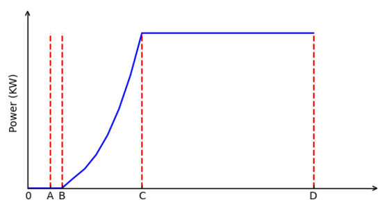
Figure 1.
The curve of wind speed and power output of direct-driven wind turbine.
(1) Shutdown stage (seen in OA and D+): This stage includes two working conditions. Working condition 1 (OA stage) means that the wind speed is below the cut-in wind speed set on the nameplate, and the wind speed at this time is not enough to start the WT. Working condition 2 (D+ stage) means the wind speed exceeds the cut-out wind speed set on the nameplate. At this moment, the wind speed is very large. From the perspective of safety and protection of the WT, the WT is forced to stop.
(2) Startup stage (seen in AB): The characteristics of the working condition in this stage is that the wind speed exceeds the cut-in wind speed. After the startup condition is satisfied, the blades are turned from the stop position to the starting position (set to 30° in our study), but the rotational speed of the hub is very low, less than the cut-in speed (set to 3.5 r/min in our study), and the WT is pre-generating.
(3) Maximum wind energy tracking stage (seen in BC): The characteristics of working condition in this stage is that the wind speed is between the cut-in wind speed and the rated wind speed. The hub speed is greater than the cut-in speed (3.5 r/min in our study) and less than the rated speed. The blades turn to the working position and remain there at all times. At this stage, the WT control system adjusts the speed of the blades according to the wind speed, keeps the optimal tip speed ratio, and maximizes the wind power utilization coefficient.
(4) Constant power stage (seen in CD): The characteristics of the working condition in this stage is that the wind speed is between the rated wind speed and the cut-out wind speed. The pitch control system adjusts the pitch angle of the blade by driving the pitch motor, variable speed gearbox, and pitch bearing, and then controls the rotational speed of the hub. The change of the pitch angle can keep the speed of the hub around the rated speed, and the output power is around the rated output power. At this time, the wind energy utilization coefficient is not the optimal value.
From the above analysis, it can be seen that the direct-drive WTs have different control strategies at different stages. Based on the data we collected from our research object of large-scale direct-drive WTs, we derived a scatter plot of wind speed and output power, as well as a distribution map of the data in the two dimensions of wind speed and output power, which are shown in Figure 2. In Figure 2, the BC stage and the CD stage are the main operating stages of WT operation. These two stages mainly involve four core parameters, namely wind speed, power, rotational speed, and pitch angle. Specifically, the main feature of the BC stage is that the rotational speed is adjusted according to the wind speed, and the pitch angle is always kept constant. In this way, the maximum wind energy utilization coefficient value is the largest, which also ensures that the WT can obtain more wind energy and power. The main feature of the CD stage is to adjust the pitch angle based on the wind speed to keep the rotation speed almost constant, the output power is always stable near the rated power, and the WT is in a full state. Therefore, like most researchers, this paper also selects the data sets of these two segments for modeling and analysis.
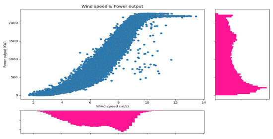
Figure 2.
The scatter and distribution of wind speed and power.
To accurately monitor and evaluate the operating condition of the main bearing, combined with our previous research results [30], there are eleven parameters that should be considered in the BC stage, namely, wind speed, ambient temperature, main bearing temperature, rotor speed, output power, generator operation frequency, generator torque, generator stator temperature, 5-s mean yaw to wind, vibration in the X direction, and vibration in the Y direction. In the CD stage, the pitch angle parameter should be added, so there are twelve parameters in this stage.
3. Proposed Condition Monitoring Model DA-Bi-LSTM
In this section, we first give the problem definition of condition monitoring of the WT main bearing. Then, we present the framework for the proposed model DA-Bi-LSTM. Finally, we design the corresponding algorithm pseudocode for training the DA-Bi-LSTM model.
3.1. Problem Definition
Under normal conditions, the condition data of the WT main bearing itself and its associated condition data will satisfy a dynamic and stable internal equilibrium relationship, with the data fluctuating within a certain range and maintaining some constraint characteristics between them. In the event of a failure of the main bearing, the dynamic equilibrium is broken. The WT main bearing condition monitoring problem can be defined as a combination of a nonlinear model and reconstruction error, which is described as follows:
where denotes sampling time, is the condition parameters describing the main bearing at the tth moment, which is the input vector of the function , especially, . is the output value of the function , which represents the reconstructed value of the condition parameters of the main bearing at the tth moment, especially, . is the number of feature parameters that characterize the operating condition of the main bearing. represents the length of the sliding window. is a row vector containing the ith condition parameter with w measured values, and is also a row vector of the ith condition parameter with w predicted values. represents a series of nonlinear mapping functions. is the reconstruction error value. Therefore, the essence of condition monitoring of the main bearing is that the reconstructed vector is as similar as possible to the input vector , with a minimum residual between the two vectors. represents the residual value. The value will exceed the threshold or alarm value if there is an abnormality or failure in the main bearing. Under normal conditions, this residual value fluctuates within the specified normal range.
3.2. Framework for the Proposed Model
The architecture of the proposed model for condition monitoring of the WT main bearing is shown in Figure 3. The architecture consists of six submodules, namely the input module, the temporal attention computation module, the parametric attention computation module, the dual attention merging module, the Bi-LSTM module, and the reconstruction module. The following subsections describe these modules in detail.
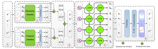
Figure 3.
The framework of the proposed model DA-Bi-LSTM. ① Input module; ② parametric attention computation module; ③ temporal attention computation module; ④ dual attention merging module; ⑤ Bi-LSTM module; ⑥ reconstruction module.
3.2.1. Input Module
For a comprehensive description of the operating condition of the main bearing, the condition parameters of the main bearing itself and the associated condition parameters should be extracted. Note that the extracted parameters will be different for different operation phases because the control strategy is different for different phases. According to the analysis in Section 2, we obtain the input condition parameters for the maximum wind energy tracking phase as an input matrix , which is defined in this form (m, w), where m is the number of variables and w is the length of the window. In this study, m is set to 11, and w is set to 5, while in the constant power phase, m is set to 12, and w is also set to 5. For the convenience of subsequent calculations, we only discuss the BC phase here. Thus, the input vector at the ith moment can be described as , where can take values in the range of 1, 2, 3, 4, and 5.
3.2.2. Parametric Attention Computation Module
In the process of parameter feature extraction, to distinguish the importance of different condition parameters, and assign different weights to different condition parameters, the parametric attention computation module can calculate the weights of the condition parameters within each time step. For the given input vector , we can use Equations (2) and (3) to compute parametric attention weight distribution values.
where represents the weight coefficient matrix, and represents the bias term, represents the sigmoid function, and is the normalized attention weight for the jth condition parameter, which is a calculation method of entropy weight, and the following is the same.
3.2.3. Temporal Attention Computation Module
The values of the condition parameters of the main bearing have a clear time series characteristic. The current value of the sequence is influenced by its historical moment value. However, the contribution or influence of different historical moment values is different. The temporal attention computation module can calculate the weights for each condition parameter over multiple consecutive time steps. For the given input vector , we can use Equations (4) and (5) to compute their temporal attention weight distribution values.
where represents the weight coefficient matrix, and represents the bias term. represents the sigmoid function, and is the normalized attention weight for the ith condition parameter.
3.2.4. Dual Attention Merging Module
To merge and fuse the temporal attention feature value and the parameter attention feature value, the dual attention merging module first calculates the temporal attention and the parametric attention by the element-wise product method separately, then, calculates the final input vector using the element-wise sum method by using Equation (6).
3.2.5. Bi-LSTM Module
The Bi-LSTM (Bi-directional Long Short-Term Memory) is a bi-directional recurrent neural network based on LSTM, which combines information from input data in both forward and backward directions, and is a variant of LSTM. The Bi-LSTM model has made remarkable achievements in speech processing, temporal data prediction, and text classification [25,31]. Figure 4 illustrates the architecture of a single LSTM cell/unit, where , , and are the forget, input, and output gates, respectively. The represents input vector. The represents the output of the previous unit at time t − 1, and represents the output of the current time t. The represents the cell state at the previous time t − 1, and represents the cell state at the current time t. The and are activation functions. These parameters at the time t are updated by:
where , , , , , , , and are weight parameters and their biases, respectively. These parameter values are obtained by iterative iterations during the DA-Bi-LSTM model training.
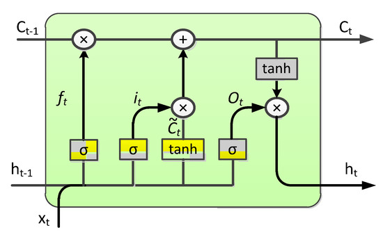
Figure 4.
The internal architecture of a single LSTM unit/cell.
The Bi-LSTM model is created by adding an LSTM layer in the opposite direction of the information flow, which has the benefit of capturing the past and future temporal dependencies. Figure 5 shows the architecture of Bi-LSTM. For the kth time point, is input to the forward and reverse LSTM, and then we get the forward and reverse hidden layer representations vectors and , respectively, and we use Equation (13) to combine these two hidden layer representations to get the output at kth time point. After the sequence is input into the Bi-LSTM, we get the final output of the module, i.e., .
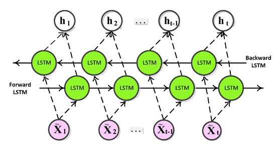
Figure 5.
The architecture of Bi-LSTM.
3.2.6. Reconstruction Module
This module is a reconstruction of the extracted feature vectors. Specifically, the output vector of Bi-LSTM is nonlinearly transformed, and then the reconstructed vector Z of the same dimension as the input vector is obtained, which is calculated by Equation (14).
where represents the weight coefficient matrix, and represents the bias term, and represents the sigmoid function. is the reconstruction vector.
3.3. Training Algorithm for the DA-Bi-LSTM Model
Based on the framework in Figure 3, an algorithm for the DA-Bi-LSTM model is proposed. The critical procedures are described as: (1) loading SCADA data in CSV files under different operating conditions in normal conditions; (2) performing data cleaning and resampling; (3) selecting the relevant condition parameter variables; (4) constructing train, verify and test datasets according to the given ratio; (5) building the proposed model DA-Bi-LSTM; (6) training the model according to the range given by the hyperparameters; (7) preserving the optimal model. A more detailed description of the training process is listed in the following pseudo-code Algorithm 1.
| Algorithm 1: Pseudo-code for DA-Bi-LSTM | |
| Input: | |
| Output: The optimal DA-Bi-LSTM model | |
| 1: | Read SCADA historical data in a normal state; |
| 2: | Clean and resample data; |
| 3: | Select condition parameter variables related to the main bearing; |
| //generate training data set, test dataset, verify data set; | |
| 4: | , TED = |
| 5: | while i in (1, n-w) do: |
| 6: | |
| 7: | end while |
| 8: | According to the ratio of 64%, 16%, and 20%, generate |
| //train DA-Bi-LSTM model | |
| 9: | Set the range of units , hidden layers , iterations , learning rate |
| , ne and batch size; | |
| 10: | Initialize parameters; |
| 11: | while i ≤ e or ne = epoch numbers when the loss has not changed: |
| 12: | Execute the temporal attention module; |
| 13: | Execute the parametric attention module; |
| 14: | Combine the values of the two attention modules; |
| 15: | Reconstruct input data; |
| 16: | Update parameters with the Adam algorithms to minimize |
| reconstruction error in ; | |
| 17: | Verify the DA-Bi-LSTM model using the ; |
| 18: | Save the structure and parameters of the optimum model; |
| 19: | end while |
| 20: | Test the model using the test dataset ; |
| 21: | Return the optimal DA-Bi-LSTM model; |
4. Experiment Setup and Result Analysis
In this section, we first probe the distribution characteristics of the relevant condition parameters of the WT main bearing based on the WT SCADA system. Second, we introduce methods for data cleaning, data resampling, and dataset construction. Third, we present the structure determination of the proposed model and the performance comparison with other models. Finally, we present the attention and interpretability analysis of the model. The experiment setup is as follows: Python 3.6 and the deep learning framework Keras API are used for experimental design.
4.1. Distribution Characteristics of Partial Conditional Parameters
In this paper, the main bearing of a 2 MW direct-drive WT is investigated. The wind turbine’s cut-in, cut-out, and rated wind speeds are 3, 25, and 11 m/s, respectively. The wind turbine is equipped with a SCADA system that collects data at 1 Hz and stores it in a 10-min CSV file. We collected data for three months, from 5 September 2020, to 4 December 2020. According to the discussion in Section 2, we extracted the continuous data of the BC segment and the CD segment. After removing the outage data, we found that the amount of data in the CD segment was relatively small, which was related to the wind conditions at that time. The wind speed is not above rated wind speed most of the time. Therefore, the following experiments were carried out on the BC stage.
Figure 6 depicts a scatter plot of some parameters associated with the WT main bearing. As shown in Figure 6, there is a heavy nonlinear relationship among the parameters. Temperature, output power, and vibration are the core parameters that characterize the operating condition of the main bearing. The temperature increases with the increase of power, but in the same output power value range, the temperature varies widely. The vibration values in the two directions also keep the range reduced with the increase of the output power, but the performance is more obvious in the axial direction (X-axis direction), and weaker in the radial direction (Y-axis direction). The complex nonlinear relationship between these parameters requires powerful nonlinear fitting functions to realize. We designed such a complex function to solve this problem.
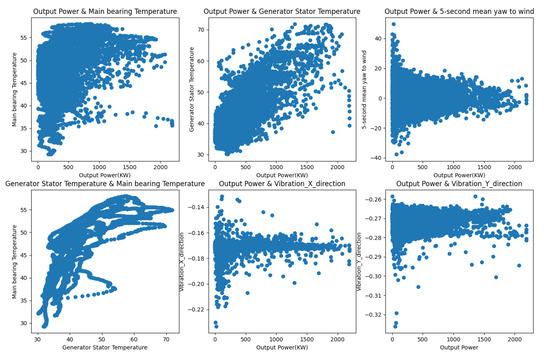
Figure 6.
The scatter diagram of partial parameters related to WT main bearing.
4.2. Data Cleansing and Resampling
Data cleaning aims to deal with invalid data such as null values and outliers in the SCADA dataset due to transmission problems and WT downtime. These invalid data are usually empty, negative data, packet loss data, and unreasonable abnormal data. Additionally, according to existing research, data resampling techniques were used [32,33]. In this study, the resampling frequency is 1 min. The processing formula is as follows:
where, represents the data value collected by sensors, which is second-level data. represents the number of data points. represents the resampled data, which is an average value.
4.3. Dataset Construction
To continuously extract the observation data and generate the training samples and test samples required by the proposed model, we use the sliding window method to process the original condition parameter data. Figure 7 shows its specific construction process, where represents the width of the sliding window, represents the sliding step size, represents a certain time point, and represents the number of condition parameters representing the main bearing. For each input vector with window length and input dimension , the input vector is denoted as .
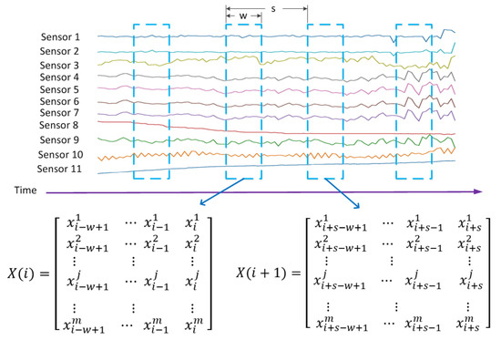
Figure 7.
Sliding window procedure for dataset construction.
4.4. Evaluation Metrics
In this paper, three different evaluation metrics are chosen to evaluate the performance of the proposed model and competitor models. The evaluation metrics are the mean absolute error (MAE), the mean absolute error percentage (MAPE), and the root mean square error (RMSE). Their calculation expressions are defined as follows:
where is the reconstructed value at the ith time. is the measured value at the ith time. is the number of sample points.
In this study, we collect 495,900 sample data. After data cleaning and resampling, the total number of samples is 8265, of which 6612 samples are used for training and 1653 samples are used for testing. Partial samples are shown in Table 1.

Table 1.
Partial samples for training and testing.
4.5. Determination of the DA-Bi-LSTM Model
Neural networks and deep learning models have certain randomness during training, such as weight initialization randomness, regularization randomness, and optimization randomness. Therefore, for the same data given, the output of the model has a certain difference. A common approach is to run the network multiple times, then some statistical methods are used to summarize the performance of the model, and finally, the best model is selected [34,35]. During the training of DA-Bi-LSTM, many hyperparameters need to be determined. Since the structure of the model designed in this paper is relatively simple, it is an auto-encoding reconstruction model, so only the learning rate and batch size need to be determined here. This paper uses the grid search method to run the model multiple times. The experimental results of some evaluation indicator values, such as MAE, MAPE, and RMSE, are shown in Table 2. It should be pointed out that the time required for the model to run is also an important evaluation indicator, and its value is given accordingly.
Table 2.
Performance indexes of different hyperparameters in DA-Bi-LSTM.
From Table 2, as the batch size increases, the metrics MAE, MAPE, and RMSE values on the test dataset tend to increase. The average proportions of batch-by-batch increase are, in terms of MAE: 11.32%, 26.21%, 36.78%, and 42.97%. In terms of MAPE: −8.96%, 4.37%, 38.04%, and 39.89%; in terms of RMSE: 12.76%, 27.04%, 36.75%, and 43.48%. The training time of the model shows a gradual downward trend. The proposed model is a reconstruction model, which is relatively simple, so it does not mean that the larger the batch size, the better, or the smaller the better. The optimal value of MAPE is reflected in the batch size of 8, not 4. In addition, although the training time of the model shows a gradual downward trend, according to the relevant selection principles, within the time range commonly used for data collection in the industry, the smaller the three evaluation metrics values, the better [8]. Therefore, our final choice is that the batch size is set at 8, and the learning rate is set at 0.005.
4.6. Performance Comparison
To compare the performance of the proposed model, three baseline models are used, such as the Bi-LSTM model, the temporal attention-based Bi-LSTM (Temporal-Att-Bi-LSTM) model, and the parameter attention-based Bi-LSTM (Parameter-Att-Bi-LSTM). All models use the same input data format, but each input data is handled differently within each model. Among them, the Bi-LSTM model is not added with an attention module, and it only considers the before and after information of the time series. The Temporal-Att-Bi-LSTM model takes into account both the temporal attention information and the before and after information of the time series. The Parameter-Att-Bi-LSTM model considers the parameter attention information and the before and after information of the time series. The comparison results are listed in Table 3 and Figure 8.
Table 3.
Performance indexes of different models (best values displayed in boldface).
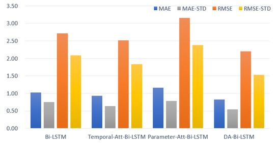
Figure 8.
Performance comparison of different models with standard deviation distribution.
In Table 3 and Figure 8, the proposed DA-Bi-LSTM model shows the best performance, followed by the Temporal-Att-Bi-LSTM model and Bi-LSTM, and the worst model is the Parameter-Att-Bi-LSTM. The MAE value and RMSE value of the proposed model, and their corresponding standard deviations, are the smallest. Specifically, compared with Bi-LSTM, Temporal-Att-Bi-LSTM, and Parameter-Att-Bi-LSTM, the MAE value of the proposed model decreases by about 19.78%, 11.79%, and 28.84%, respectively. The standard deviation of the MAE values of the proposed model is lower than 22.77%, 15.31%, and 30.67%, respectively. Compared with Bi-LSTM, Temporal-Att-Bi-LSTM, and Parameter-Att-Bi-LSTM, the RMSE values of the proposed model drop by about 18.92%, 12.55%, and 30.37%, respectively. The standard deviation of the RMSE value of the proposed model is lower than 26.62%, 16.66%, and 35.53%, respectively. The MAPE values of all models are around 0.055, and the discrimination is not obvious because MAPE is the mean of the relative percentage of the reconstruction error to the measured value.
In Figure 8, the Parameter-Att-Bi-LSTM model that only considers parameter attention is worse than the Bi-LSTM model because the model assigns different weights to different parameters before extracting the information before and after the time series, ignoring weak timing information for unimportant parameters. So, its effect is worse than the Bi-LSTM model. The Temporal-Att-Bi-LSTM model works better than Bi-LSTM because our data itself is time series data, and the time series attention module further highlights the importance of the data at different times. The DA-Bi-LSTM model performs the best because it integrates time-series attention information and parameter attention information, the time-series information of important parameters, and the weak time-series information of non-important parameters, which are all included. Specifically, the DA-Bi-LSTM model emphasizes the extraction of the importance of different input parameters and the extraction of parameter time series features. Then, the extracted information from the two aspects is further fused, and the time series features of the composite information are finally extracted and learned. Therefore, its information representation and extraction ability are the strongest, and the effect is also the best.
4.7. Attention and Interpretability Analysis
The attention mechanism module in the proposed model can give the dynamic attention score of each parameter of each input sample to the operating condition of the main bearing in real time and can reflect the contribution of different time points and different parameter variables to the main bearing in real time. In a heatmap of attention scores, the darker the color, the higher the attention value, and vice versa.
In the parametric attention score calculation module, we extract the parametric attention score value of a sample, as shown in Figure 9. Where the horizontal coordinate, X-axis, represents different time points, the vertical coordinate, Y-axis, represents 11 condition parameters, and the numbers in the figure represent the contribution of parameter attention. The attention score of each condition parameter variable is different. Vibration in two directions and “5 s mean yaw wind” are important parameters, especially in the Y direction. However, the degree of influence for some parameters such as temperature is not as obvious. Specifically, the attention score of “Y vibration value” is the largest, accounting for about 17.72% on average, and it is maintained, followed by “5 s mean yaw wind”, “X vibration”, “average temperature of generator stator”, and “wind speed”, which accounted for 13.09%, 12.13%, 10.52%, and 9.73%, respectively. The lowest attention scores are “average temperature of the main bearing” and “power output”, which are 4.36% and 4.42%, respectively. The parameter attention calculation module can select some parameter variables and can assign different attention scores to these parameters according to the speed of parameter change and the constraint relationship between parameters in the actual process of monitoring.
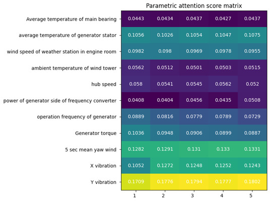
Figure 9.
A heatmap of parametric attention scores.
In the temporal attention score calculation module, we also extract the temporal attention score value of a sample, as shown in Figure 10, where the horizontal coordinate represents different time points, the vertical coordinate represents 11 condition parameters, and the numbers in the figure represent the contribution of the temporal attention score. Relative to time t, most of the temporal attention scores are highest at time t − 1 and time t − 3, accounting for about 20.23% and 20.14%, respectively. The most obvious one is “wind speed”, accounting for 20.6%, followed by “generator torque”, accounting for 20.47%, followed by “power output” and “5-s mean yaw to wind”, accounting for 20.35% and 20.3%, respectively. The temperature parameter is a gradually changing quantity. However, the time-series attention score distribution of temperature parameters still has differences in the main bearing and related components parameters. The attention score distribution of the temperature of the main bearing itself is relatively balanced at about 20%, at times t − 2 and t − 4, the proportion is larger, showing a high in the middle and low at both ends. However, there is no obvious regularity in the changes of the generator stator temperature parameters and the external environment temperature parameters, and the standard deviation of its attention score is the lowest, 0.0011. The standard deviation of attention scores for the vibration parameter of “vibration in X direction” was the largest, followed by the wind speed parameter, which was 0.008 and 0.0057, respectively. This also shows that the wind speed fluctuates greatly, and the X-axis fluctuates greatly. The temporal attention calculation module can select different time points and can assign different attention scores to different historical time points, emphasizing the expression of key information at important time points.
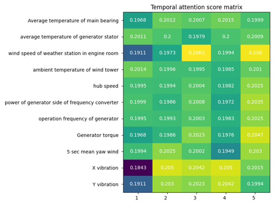
Figure 10.
A heatmap of temporal attention scores.
5. Conclusions
This work presents a novel method of condition monitoring for WT main bearing by using the dual attention mechanism and Bi-LSTM. The effectiveness of the proposed method is verified by using the WT SCADA data. The research results show that the proposed model for the different working conditions can further exactly explore the spatiotemporal correlation between the condition parameters of the WT main bearing itself and its associated condition parameters, strengthen the key information in the input data, weaken the secondary information, and improve the precision of the main bearing condition monitoring and the interpretability of the monitoring model.
In the future, we will further expand the verification and application of the proposed model in the constant power stage, and also include the modeling of the model on other key components or subsystems, such as generators, hubs, pitch systems and yaw systems, etc. At the same time, we will also consider field testing and deployment of the proposed method for better monitoring and earlier warning of WT main bearing failures.
Author Contributions
The research in this paper was the result of the joint efforts of all authors. X.X.: methodology, software, validation, writing—original draft preparation; J.L.: conceptualization, supervision, writing—reviewing and editing, funding acquisition; D.L.: conceptualization, supervision, writing—reviewing and editing, funding acquisition; Y.T.: conceptualization, supervision, writing—reviewing; S.Q.: validation, visualization; F.Z.: validation. All authors have read and agreed to the published version of the manuscript.
Funding
This research was funded by National Key R&D Program of China, grant number 2020YFB1707602, the National Natural Science Foundation of China, grant number 51475160, and the Key Research and Development Project of Hunan Province, China, grant number 2018WK2022.
Data Availability Statement
The datasets used in the current study are available from the corresponding author upon reasonable request.
Conflicts of Interest
The authors declare no conflict of interest.
References
- Brodny, J.; Tutak, M.; Bindzár, P. Assessing the level of renewable energy development in the European union member states. A 10-year perspective. Energies 2021, 14, 3765. [Google Scholar] [CrossRef]
- Li, J.; Ho, M.S.; Xie, C.; Stern, N. China’s flexibility challenge in achieving carbon neutrality by 2060. Renew. Sustain. Energy Rev. 2022, 158, 112112. [Google Scholar] [CrossRef]
- Yang, Q.; Liu, G.; Bao, Y.; Chen, Q. Fault Detection of Wind Turbine Generator Bearing Using Attention-Based Neural Networks and Voting-Based Strategy. IEEE/ASME Trans. Mechatron. 2021, 27, 3008–3018. [Google Scholar] [CrossRef]
- Xiang, L.; Yang, X.; Hu, A.; Su, H.; Wang, P. Condition monitoring and anomaly detection of wind turbine based on cascaded and bidirectional deep learning networks. Appl. Energy 2022, 305, 117925. [Google Scholar] [CrossRef]
- Civera, M.; Surace, C. Non-Destructive Techniques for the Condition and Structural Health Monitoring of Wind Turbines: A Literature Review of the Last 20 Years. Sensors 2022, 22, 1627. [Google Scholar] [CrossRef]
- Hart, E.; Clarke, B.; Nicholas, G.; Kazemi Amiri, A.; Stirling, J.; Carroll, J.; Dwyer-Joyce, R.; McDonald, A.; Long, H. A review of wind turbine main bearings: Design, operation, modelling, damage mechanisms and fault detection. Wind Energy Sci. 2020, 5, 105–124. [Google Scholar] [CrossRef]
- Gbashi, S.M.; Madushele, N.; Olatunji, O.O.; Adedeii, P.A.; Jen, T.-C. Wind Turbine Main Bearing: A Mini Review of Its Failure Modes and Condition Monitoring Techniques. In Proceedings of the 2022 IEEE 13th International Conference on Mechanical and Intelligent Manufacturing Technologies (ICMIMT), Cape Town, South Africa, 25–27 May 2022; pp. 127–134. [Google Scholar]
- Hart, E. Developing a systematic approach to the analysis of time-varying main bearing loads for wind turbines. Wind Energy 2020, 23, 2150–2165. [Google Scholar] [CrossRef]
- Nejad, A.R.; Keller, J.; Guo, Y.; Sheng, S.; Polinder, H.; Watson, S.; Dong, J.; Qin, Z.; Ebrahimi, A.; Schelenz, R. Wind turbine drivetrains: State-of-the-art technologies and future development trends. Wind Energy Sci. 2022, 7, 387–411. [Google Scholar] [CrossRef]
- Hart, E.; Turnbull, A.; Feuchtwang, J.; McMillan, D.; Golysheva, E.; Elliott, R. Wind turbine main-bearing loading and wind field characteristics. Wind Energy 2019, 22, 1534–1547. [Google Scholar] [CrossRef]
- Tutivén, C.; Vidal, Y.; Insuasty, A.; Campoverde-Vilela, L.; Achicanoy, W. Early Fault Diagnosis Strategy for WT Main Bearings Based on SCADA Data and One-Class SVM. Energies 2022, 15, 4381. [Google Scholar] [CrossRef]
- Encalada-Dávila, Á.; Puruncajas, B.; Tutivén, C.; Vidal, Y. Wind Turbine Main Bearing Fault Prognosis Based Solely on SCADA Data. Sensors 2021, 21, 2228. [Google Scholar] [CrossRef] [PubMed]
- Natili, F.; Daga, A.P.; Castellani, F.; Garibaldi, L. Multi-Scale Wind Turbine Bearings Supervision Techniques Using Industrial SCADA and Vibration Data. Appl. Sci. 2021, 11, 6785. [Google Scholar] [CrossRef]
- Beretta, M.; Julian, A.; Sepulveda, J.; Cusidó, J.; Porro, O. An Ensemble Learning Solution for Predicitive Manintenance of Wind Turbines Main Bearing. Sensors 2021, 21, 1512. [Google Scholar] [CrossRef] [PubMed]
- Guo, P.; Wang, Z. Wind turbine spindle state monitoring based on Gaussian process regression and double moving window residual processing. Electr. Power Autom. Equip. 2018, 38, 34–40. [Google Scholar] [CrossRef]
- Beretta, M.; Vidal, Y.; Sepulveda, J.; Porro, O.; Cusidó, J. Improved ensemble learning for wind turbine main bearing fault diagnosis. Appl. Sci. 2021, 11, 7523. [Google Scholar] [CrossRef]
- Zheng, Y.; Wei, J.; Zhu, K.; Bo, D. Fault Monitoring Method of Wind Turbine Main Bearing. J. Vib. Meas. Diagn. 2021, 41, 341–347 + 415. [Google Scholar] [CrossRef]
- Liu, C.; Duan, B.; Xiaodan, Z. An abnormal identification method for the main bearing of wind turbines based on BPNN-NCT. Power Syst. Prot. Control 2022, 50, 114–122. [Google Scholar] [CrossRef]
- Zhang, Y.; Zheng, H.; Liu, J.; Zhao, J.; Sun, P. An anomaly identification model for wind turbine state parameters. J. Clean. Prod. 2018, 195, 1214–1227. [Google Scholar] [CrossRef]
- Xu, Z.; Yang, P.; Zhao, Z.; Lai, C.S.; Lai, L.L.; Wang, X. Fault diagnosis approach of main drive chain in wind turbine based on data fusion. Appl. Sci. 2021, 11, 5804. [Google Scholar] [CrossRef]
- Tutiv’en, C.; Benalcazar–Parra, C.; D’avila Escuela, A.E.; Vidal, Y.; Puruncaias, B.; Fajardo, M. Wind Turbine Main Bearing Condition Monitoring via Convolutional Autoencoder Neural Networks. In Proceedings of the 2021 International Conference on Electrical, Computer, Communications and Mechatronics Engineering (ICECCME), Mauritius, 7–8 October 2021; pp. 1–6. [Google Scholar]
- Tonks, O.; Wang, Q. The detection of wind turbine shaft misalignment using temperature monitoring. J. Manuf. Sci. Technol. 2017, 17, 71–79. [Google Scholar] [CrossRef]
- Yucesan, Y.A.; Viana, F.A. A hybrid physics-informed neural network for main bearing fatigue prognosis under grease quality variation. Mech. Syst. Signal Process. 2022, 171, 108875. [Google Scholar] [CrossRef]
- Rezamand, M.; Kordestani, M.; Orchard, M.E.; Carriveau, R.; Ting, D.S.-K.; Saif, M. Improved remaining useful life estimation of wind turbine drivetrain bearings under varying operating conditions. IEEE Trans. Ind. Inform. 2020, 17, 1742–1752. [Google Scholar] [CrossRef]
- Zheng, Y.-F.; Gao, Z.-H.; Shen, J.; Zhai, X.-S. Optimising Automatic Text Classification Approach in Adaptive Online Collaborative Discussion-A perspective of Attention Mechanism-Based Bi-LSTM. IEEE Trans. Learn. Technol. 2022, 1–14. [Google Scholar] [CrossRef]
- Yin, X.; Wu, G.; Wei, J.; Shen, Y.; Qi, H.; Yin, B. Multi-stage attention spatial-temporal graph networks for traffic prediction. Neurocomputing 2021, 428, 42–53. [Google Scholar] [CrossRef]
- Hu, J.; Zheng, W. Multistage attention network for multivariate time series prediction. Neurocomputing 2020, 383, 122–137. [Google Scholar] [CrossRef]
- Su, X.; Shan, Y.; Li, C.; Mi, Y.; Fu, Y.; Dong, Z. Spatial-temporal attention and GRU based interpretable condition monitoring of offshore wind turbine gearboxes. IET Renew. Power Gener. 2022, 16, 402–415. [Google Scholar] [CrossRef]
- Xiang, L.; Wang, P.; Yang, X.; Hu, A.; Su, H. Fault detection of wind turbine based on SCADA data analysis using CNN and LSTM with attention mechanism. Measurement 2021, 175, 109094. [Google Scholar] [CrossRef]
- Xiao, X.; Liu, J.; Liu, D.; Tang, Y.; Dai, J.; Zhang, F. SSAE-MLP: Stacked sparse autoencoders-based multi-layer perceptron for main bearing temperature prediction of large-scale wind turbines. Concurr. Comput. Pract. Exp. 2021, 33, e6315. [Google Scholar] [CrossRef]
- Zhang, H.; Huang, H.; Han, H. A Novel Heterogeneous Parallel Convolution Bi-LSTM for Speech Emotion Recognition. Appl. Sci. 2021, 11, 9897. [Google Scholar] [CrossRef]
- Cambron, P.; Masson, C.; Tahan, A.; Pelletier, F. Control chart monitoring of wind turbine generators using the statistical inertia of a wind farm average. Renew. Energy 2018, 116, 88–98. [Google Scholar] [CrossRef]
- Xiao, X.; Liu, J.; Liu, D.; Tang, Y.; Zhang, F. Condition Monitoring of Wind Turbine Main Bearing Based on Multivariate Time Series Forecasting. Energies 2022, 15, 1951. [Google Scholar] [CrossRef]
- Pei, S.; Qin, H.; Yao, L.; Liu, Y.; Wang, C.; Zhou, J. Multi-step ahead short-term load forecasting using hybrid feature selection and improved long short-term memory network. Energies 2020, 13, 4121. [Google Scholar] [CrossRef]
- Hossain, M.A.; Chakrabortty, R.K.; Elsawah, S.; Ryan, M.J. Very short-term forecasting of wind power generation using hybrid deep learning model. J. Clean. Prod. 2021, 296, 126564. [Google Scholar] [CrossRef]


Publisher’s Note: MDPI stays neutral with regard to jurisdictional claims in published maps and institutional affiliations. |
© 2022 by the authors. Licensee MDPI, Basel, Switzerland. This article is an open access article distributed under the terms and conditions of the Creative Commons Attribution (CC BY) license (https://creativecommons.org/licenses/by/4.0/).