Modeling and Measuring Thermodynamic and Transport Thermophysical Properties: A Review

Abstract

The present review describes the up-to-date state of the evaluation of thermophysical properties (TP) of materials with three different procedures: modeling (also including inverse problems), measurements and analytical methods (e.g., through computing from other properties). Methods to measure specific heat and thermal conductivity are described in detail. Thermal diffusivity and thermal effusivity are a combination of the previously cited properties, but also for these properties, specific measurement and calculation methods are reported. Experiments can be carried out in steady-state, transient, and pulse regimes. For modeling, special focus is given to the inverse methods and parameter estimation procedures, because through them it is possible to evaluate the thermophysical property, assuring the best practices and supplying the measurement uncertainty. It is also cited when the most common data processing algorithms are used, e.g., the Gauss–Newton and Levenberg–Marquardt least squares minimization algorithms, and how it is possible to retrieve values of TP from other data. Optimization criteria for designing the experiments are also mentioned.

1. Introduction

The present review has the goal of highlighting the relevance of the inverse techniques in thermophysical property (TP) measurements, which is not sufficiently handled in other reviews. Furthermore, while, to the author’s knowledge, most recent reviews focus on methods devoted to measure specific materials or applications, the present review tries to provide a general overview and up-to-date the state of the art description of the main available methods for TP measurements.

Thermophysical properties are characteristic material quantities that are temperature-dependent and influence the thermal behavior of materials and components. They are divided into two main categories:

–

Thermodynamic properties, i.e., specific heat c_p, linear thermal expansion (not considered in the present review), and density $\rho$ (dependent on this last property);

–

Transport properties, i.e., transport of heat (thermal conductivity k), transport of momentum (thermal viscosity, not handled in the present review), transport of electromagnetic radiation (radiative properties, not handled here).

Furthermore, other properties are a combination of the before-mentioned properties, such as thermal diffusivity $\alpha$, which is a combination of thermal conductivity, density, and specific heat, according to the equation:

$$\alpha =\frac{k}{\rho \cdot c_p}.$$

(1)

An accurate evaluation of all these properties is fundamental to explaining thermal phenomena and describing the behavior of thermal devices and components, such as insulating materials, heat exchangers, buried pipes, geothermal heat pumps, nuclear waste recovery, etc. Additionally, the thermal behavior of non-traditional materials must be investigated through the knowledge of their thermophysical properties, such as biological materials (tissues, bones, fat, blood, foods, etc.), two-dimensional materials (e.g., graphene), composites, and so on.

Some materials exhibit non-isotropic or inhomogeneous behavior, which can heavily influence the values and measuring methods of the thermophysical properties. This is the case, for instance, of the thermal conductivity, which can be strongly dependent on the heat propagation direction. Materials of this type are, for instance, single crystals, composites, and organic fiber materials. As a consequence, the thermal diffusivity, Equation (1), can only be defined for isotropic and homogeneous materials.

Evaluation of the thermophysical properties can be carried out with three different procedures:

• Theoretically, through specific models (e.g., inverse problems);
• Experimentally, with properly designed devices and experimental procedures;
• Analytically, from the knowledge of other properties (such as thermal diffusivity or thermal effusivity).

Experimental methods, on their own, can be divided into steady-state methods, transient methods, and pulse methods. Some methods allow the contemporary measurement of more quantities, for instance, thermal conductivity and thermal diffusivity, but attention must be paid to avoid the mutual correlation among them.

The present review is organized as follows. Methods to measure, individually, specific heat, thermal conductivity, and thermal diffusivity are discussed and reviewed in Section 2, Section 3 and Section 4, respectively. Particular emphasis is placed on methods related to thermal conductivity measurements, such as the steady-state guarded hot ring and guarded hot plate methods (Section 3.1), the transient hot wire method (Section 3.2), and the thermal conductivity probe method (Section 3.3). Regarding the thermal diffusivity measurements, the laser flash method is handled in Section 4.1 and Section 4.2, the dual-probe method in Section 4.3, photothermal methods in Section 4.4, and the thermal waving source method in Section 4.5.

Additionally, in Section 5, contemporary measurements of different properties are discussed. In particular, multiple property measurements with the flash method are reviewed in Section 5.1, as well as the transient hot strip method (Section 5.2) and the transient plane source method (Section 5.3). Finally, special focus is given to the inverse transient techniques, discussing both modeling the thermal phenomena occurring in particular devices (Section 5.4) and the criteria to design optimal experiments to ensure reliable and reasonable estimates of the investigated properties (Section 5.5).

2. Specific Heat

Thermal capacity C, or specific heat c_p, defined as the specific thermal capacity per unit mass, is the thermodynamic property of materials that indicates their capacity of absorbing (or releasing) heat. Thus, its definition is the heat necessary to raise the temperature of the body by 1 °C (specific heat is the heat necessary to raise the temperature of 1 kg of matter by 1 °C).

Measurements of specific heat are carried out with calorimetric devices. The most used is thermal analysis, through specific instruments, called DTA (differential thermal analysis [1], e.g., the Mettler Toledo thermobalance) or DSC (differential scanning calorimeter [2], e.g., the Perkin Elmer system). Both systems are made of two equal samples, one containing the material to be tested, and the other a reference material, whose specific heat is known. In the DTA system, both samples are located in a furnace, whose temperature increases linearly with time. Thermal capacity is calculated from this temperature increase, and from that of the reference sample. The device requires a proper calibration with other reference samples. In the DSC system, each of the two samples have a small furnace underneath, and the heat supplied to one of the two samples to cancel the temperature difference between the two is recorded. Therefore, this last system directly supplies the value of the thermal capacity.

The sizes of the samples are very small (even few milligrams), so extra care must be taken to assure the cleanness of the sample holders and of the measuring chamber. Almost any kind of materials can be tested, in different temperature ranges and atmospheres. Only gases require specific devices, which are sealed in order to preserve them. In addition to thermal capacity, thermal analysis is also used to study chemical reaction heat production, phase transitions, and any phenomena that can influence the thermal behavior of the material.

Specific heat is important to derive thermal conductivity from the value of thermal diffusivity through Equation (1).

3. Thermal Conductivity

This property is defined as the proportionality constant between the heat flux per unit area supplied to the sample and the obtained temperature gradient, as described by Fourier’s law:

$$\overrightarrow{\dot{q}}=\frac{\dot{Q}}{\overrightarrow{A}}=-k\overrightarrow{\nabla }T,$$

(2)

where $\overrightarrow{\nabla }T$ is the temperature gradient in the heat propagation direction, and $\overrightarrow{A}$ is the area through which heat is transferred. Both $\overrightarrow{\nabla }T$ and $\overrightarrow{A}$ being vectors, their product is generally a tensor, with nine components in three-dimensional space. It is reduced to a scalar only if $\overrightarrow{\nabla }T$ and $\overrightarrow{A}$ are parallel, as in the case of isotropic materials. When the material is inhomogeneous, the value of k is also space-dependent, so most of the time the measurement procedure gives an average value. Measurement methods are steady-state or transient. The first is a direct application of Equation (2): the “guarded hot plate” and the “guarded hot ring” methods belong to this category. Transient hot strip, transient hot wire, thermal conductivity probe, and the laser flash methods belong to the second (transient) group.

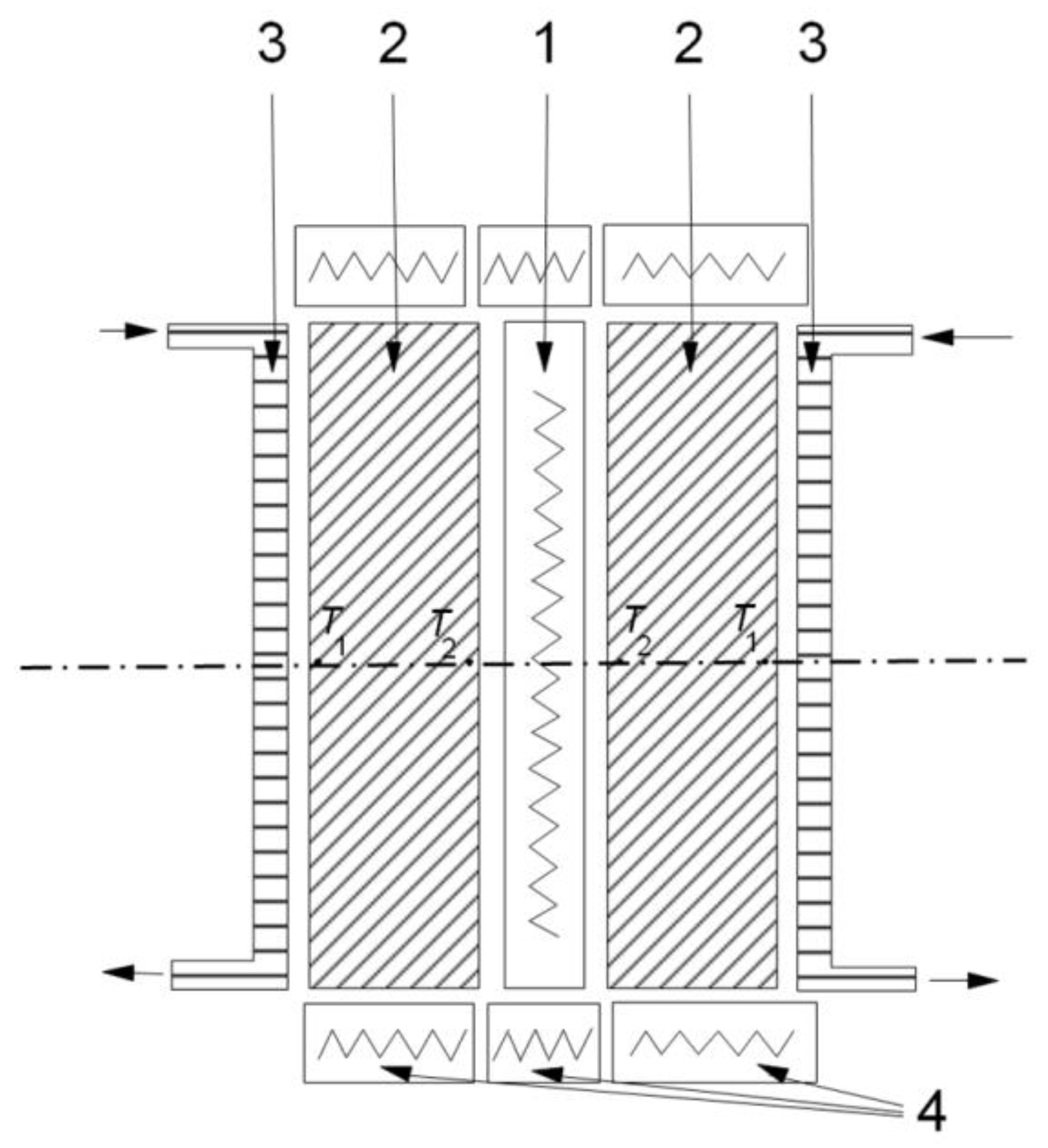
3.1. Guarded Hot Ring and Guarded Hot Plate

Even if the measurement principle is the same, the first group uses Cartesian geometry (see Figure 1) [3,4], while the second uses cylindrical geometry [5]. For the first, the sample has the form of a slab, and a sandwich is assembled, consisting of the heater, the sample, and a hot sink (e.g., a water circulation circuit). Two temperature sensors are located in the sample at distances x₁ and x₂ from the sample surface, and directly applying Equation (2), the value of k is provided.

$$k=\frac{\dot{q}}{\frac{T_1-T_2}{x_2-x_1}}.$$

(3)

A guarded ring, from which the method takes its name, is located around the whole sandwich to avoid lateral heat fluxes, which could influence the measured values.

The heater must be accurately insulated from the outside, or, better still, the sandwich is formed by two equal sequences, with the heater located in the middle (Figure 2). Both the temperature differences and the sensor positions are averaged between the two layers.

Due to the difficulty in measuring the heat flux of the heater, it is preferable that the sandwich is made of two layers (Figure 3), one containing the material to be tested, and the other a material whose k is known (k_ref). In this case, the result is obtained as follows:

$$k=k_{ref}\frac{x_2-x_1}{x_{2ref}-x_{1ref}}\frac{T_{1ref}-T_{2ref}}{T_1-T_2}.$$

(4)

The guarded hot plate [6] simply modifies the geometry in order to possess cylindrical symmetry (Figure 4). The guarded hot ring is substituted by two plates located below and over the sandwich, from which derives the name of the method. In this case, the thermal conductivity is given by the following equation:

$$k=k_{ref}\frac{\ln r_2/r_1}{\ln r_{2ref}/r_{1ref}}\frac{T_{1ref}-T_{2ref}}{T_1-T_2}.$$

(5)

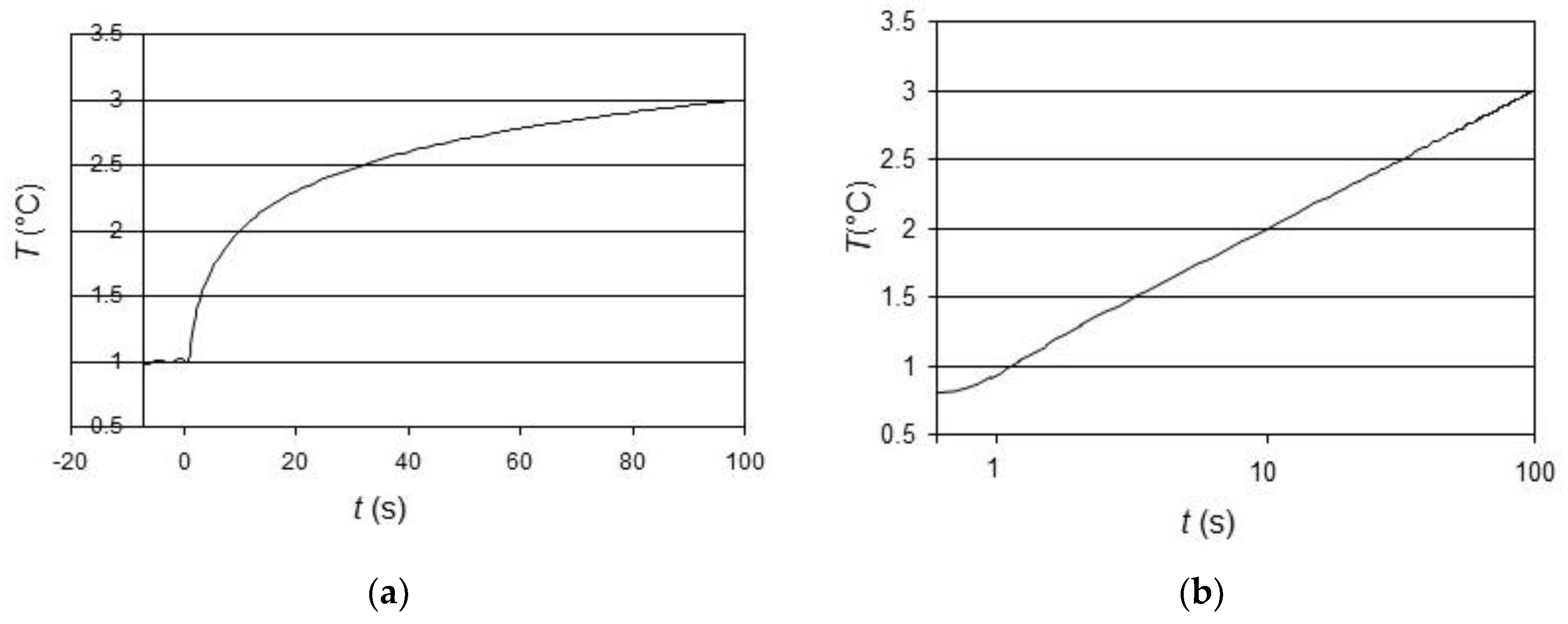
3.2. Transient Hot Wire

The transient hot wire (THW) method described by Healy et al. [7] is suited to measuring the thermal conductivity of conventional fluids, including nanofluids [8,9,10,11], and also solids. A thin electrically heated wire is immersed in the fluid sample, or inserted through a thin hole in the solid sample. This wire is subjected to a sudden constant current flow, generating a step-function-shaped thermal flux.

The THW method can be applied to isotropic materials with a thermal conductivity less than 15 W/m·K, and for temperatures ranging from cryogenic to 1500 °C [12], according to the used materials of the experimental apparatus and heating or cooling devices annexed for thermostating.

Under the hypotheses of infinite wire length and infinitesimal radius, the temperature rise in the wire is given by the following equation [13]:

$$\Delta T=-\frac{\dot{q}}{4\pi k}\mathrm{Ei}\left(-\frac{r^2}{4\alpha t}\right),$$

(6)

where $\dot{q}$ is the heat flow per unit length supplied to the wire, k the thermal conductivity, and Ei is the exponential inverse function:

$$-\mathrm{Ei}\left(-x\right)={\displaystyle \underset{x}{\overset{\infty }{\int }}\frac{e^{-x}}{x}dx={\mathrm{E}}_1(x)}.$$

(7)

For long periods of time t, i.e., for $r^2/4\alpha t<<1$, Equation (6) can be expanded in series for long time periods and, keeping only the first two terms, $\Delta T$ is given by [13,14,15,16]

$$\Delta T=\frac{\dot{q}}{4\pi k}\left(-0.5772+\ln \frac{4\alpha t}{r^2}\right),$$

(8)

0.5772 is the Euler constant.

Even if two temperature measurements T₁ and T₂ at different times t₁ and t₂ are, in principle, sufficient to estimate k with the equation

$$k=\frac{\dot{q}}{4\pi }\frac{\ln \left(t_2\right)-\ln \left(t_1\right)}{T_2-T_1},$$

(9)

a linear regression of $\Delta T$ versus the logarithm of t is preferable, because it supplies the best estimate of the slope, whichis proportional to the inverse of k, and its uncertainty.

An analytic solution of the conduction heat transfer equation also exists for finite-thickness wires [17] (pp. 339–343), but again, the series expansion of this solution, approximated for long time periods at the first order, gives a linear dependence of the temperature rise versus the logarithm of time, whose slope is inversely proportional to the thermal conductivity of the tested medium [18].

A typical trend of the detected temperature of the wire is reported in Figure 5, in Cartesian coordinates (Figure 5a) and in logarithmic form (Figure 5b).

Furthermore, through the $\Delta T$ versus log t plot, it is possible to accurately determine the deviation of the trend from the linear behavior, which occurs for different reasons:

• At the beginning, immediately after the power is switched on, the series expansion is not yet valid, so temperature gradually increases. Theoretically, this part of the trend could be used to measure the thermal capacity of the sample, but often it is much more influenced by the thermal capacity of the wire, or the thermal resistance between the sample and the wire in the case of solid samples. Moreover, this thermal resistance can often be neglected because the wire plus the fluid between the wire and the sample simply behaves as a wider wire, at least when the contact resistance is uniform along the wire length.
• At the end of the test, often the linear trend bends until it reaches a constant value. This is mainly due the beginning of convection in the sample (if fluid) or at the sample border. Clearly, only the linear portion of the curve must be considered in the data processing. In the case of solid samples, it is advisable to locate a temperature sensor (e.g., a thermocouple) at the border sample that indicates when the thermal wave reaches the end of the sample, and to neglect the data after this point. Additionally, some precautions can be taken, e.g., to expand the linear range in special cases. For example, [19] applied different magnetic fields to increase the linear range and delay the natural convection start.
• Inhomogeneous samples can exhibit a waving trend due to different heat transfer velocities in different zones of the sample.
• The so-called “wall effect” occurs when a porous medium is measured, providing the sizes of the particles of the medium are greater than the wire diameter. In this case, the method will possibly supply the value of the interstitial fluid rather than the whole porous medium.

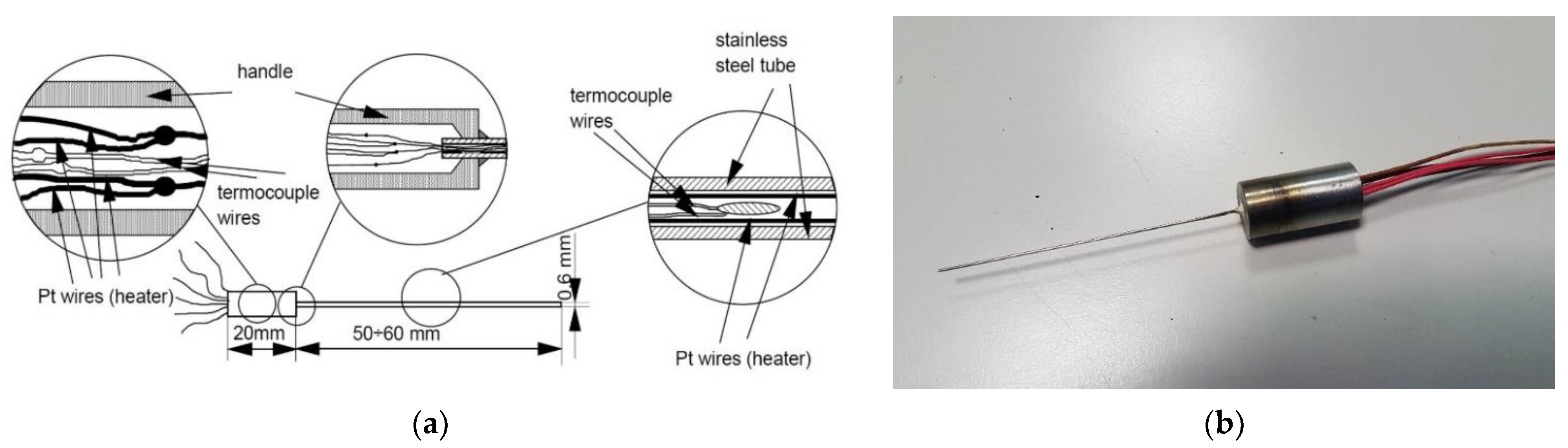
3.3. Thermal Conductivity Probe

This method is a modification of the THW: a metallic wire is folded and inserted into a stainless steel pipe with a small external diameter (0.3 ÷ 1.5 mm) [18,20]. So it appears as a bifilar wire with the two tips at the same end. Therefore, the wire length must be at least two times that of the probe, being the wire inserted bifilarly. To respect the infinite length assumption, a ratio between probe length and its external diameter l/d greater than 50 (better still, 100) must be guaranteed [13]. The wire is connected to the power supply as a four-wire resistance, so as to precisely measure the wire resistance R_w during the test, and from it the power per unit length supplied to the wire $\dot{q}=R_w{I}^2/2l$, with I representing the electric current supplied to the wire. A fluid material (e.g., epoxy resin before curing) is poured into the pipe to fill it and reduce the thermal resistance between the wire and the pipe, which could be variable from point-to-point and thus influencing the $\Delta T$ vs. lnt slope. To precisely measure the wire temperature, the wire resistance as a function of temperature can be used; however, it is preferable to insert a thin thermocouple into the middle of the probe between the two folds of the wire to avoid the variable temperature at the wire borders, near the probe ends, i.e., the handle and the tip. Figure 6a,b report a scheme of the probe construction and an image of the manufactured probe. The main advantage of this modification of the THW is the possibility to insert the probe in a generic sample through a suited hole (for solid samples), and only from one side, thus also allowing its application in field tests. However, care must be taken to assure the sample thermal uniformity, though proper thermostatic control, otherwise the linearity of the $\Delta T$ versus log t trend can be modified, and measurement uncertainty may increase. Liquids, soils, and also biological tissues have been measured with this technique [21,22].

4. Thermal Diffusivity Measurement

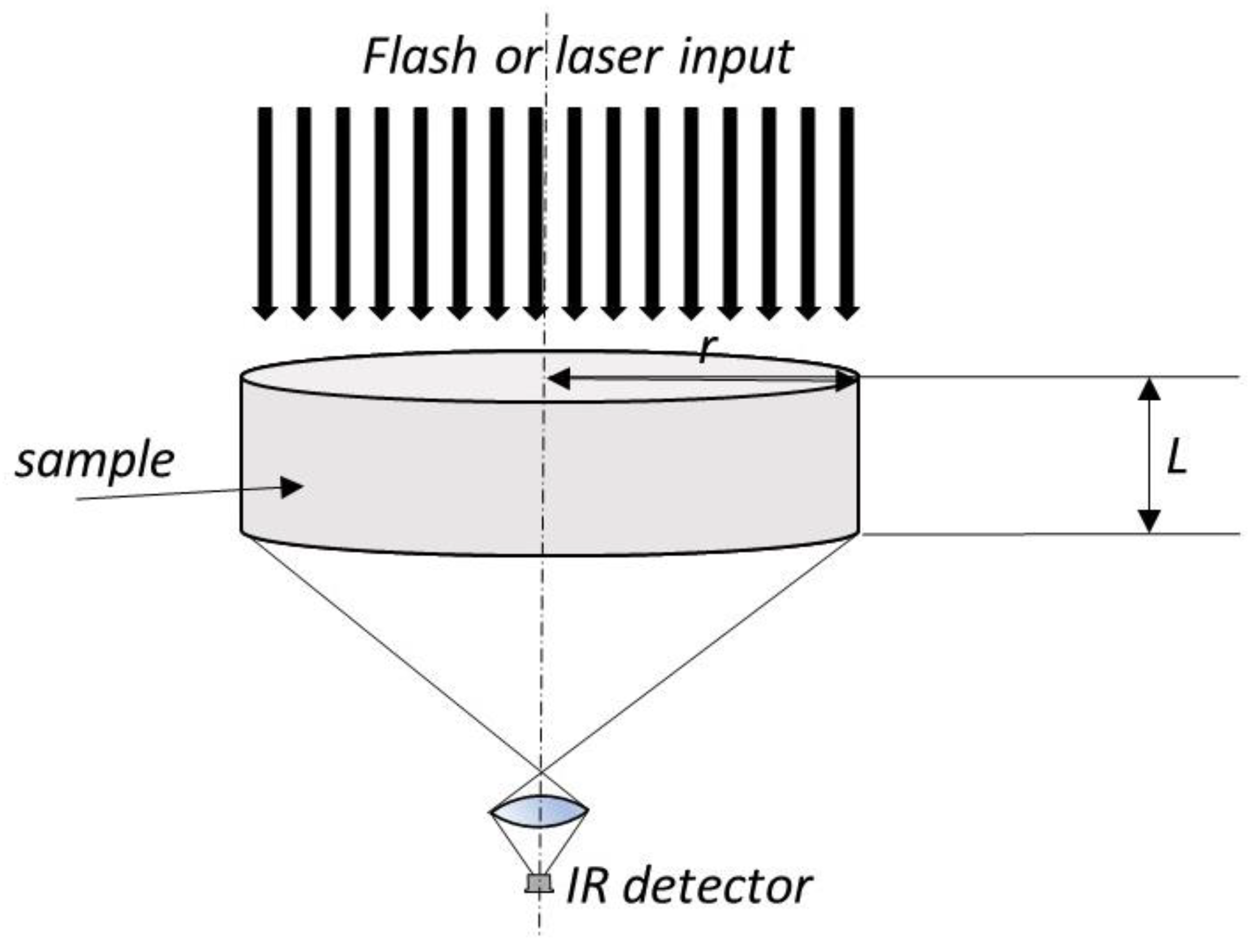
4.1. Laser Flash Method

The laser flash method described by Parker et al. [23] is widely used to measure the thermal diffusivity of homogenous, isotropic, and opaque solid materials. In fact, diffusivity values from 1 × 10⁻⁷ to 1 × 10⁻³ m²/s can be measured over a wide temperature range (from 75 to 2800 K) [12]. In this method, the front surface of a disk-shaped sample (several millimeters thick) is subjected to an energy pulse, as shown in Figure 7; as a result, the rear surface temperature increases.

This temperature can be measured via an infrared (IR) detector [24] or a thermocouple welded to the sample [25], or an open thermocouple whose terminals are placed in contact with the sample surface. Then, parameter estimation procedures, such as the Gauss method [26], Levenberg–Marquardt method [27], and similar, are used to estimate the thermal diffusivity.

In particular, when the heat losses are neglected and an instantaneous, uniform pulse is applied, the conduction within the specimen can be considered one-dimensional. Therefore, the temperature distribution in the sample, as a function of position x and time t, is given by [28]:

$$T=T_0+\frac{Q}{\rho cL}\left[1+2{\displaystyle \sum _{n=1}^{\infty }\cos \left(n\pi \tilde{x}\right)}{e}^{-n^2{\pi }^2\tilde{t}}\right],$$

(10)

where $\tilde{x}=x/L$, $\tilde{t}={\alpha t/L}^2$, Q is the energy of the pulse, and $\rho$, c_p, and L are density, specific heat, and thickness of the sample, respectively. Equation (10) is calculated for x = L to compare the analytical solution with the measured temperature of the rear of the sample. Instead of a laser, a photographic flash can be used. With respect to the laser, the spatial uniformity is higher, but the time length of the pulse is also higher, so a meaningful difference between the heat propagation time in the sample and the pulse length must be guaranteed. Figure 8 reports a view of the experimental apparatus.

However, in the reality of the experiments, the laser pulse and the photographic flash have finite time lengths or are non-uniform, and convection can occur between the sample and the environment; consequently, the heat conduction within the specimen is described by a two-dimensional model. In order to consider a finite pulse, several corrections have been suggested, and other heat transfer parameters in addition to thermal diffusivity must be considered [28,29,30].

Figure 8. Photograph of the experimental apparatus of the flash method used in [30]: (1) photographic flash; (2) detector power supply; (3) IR detector with its Dewar; (4) sample; (5) detector signal amplifier.

Figure 8. Photograph of the experimental apparatus of the flash method used in [30]: (1) photographic flash; (2) detector power supply; (3) IR detector with its Dewar; (4) sample; (5) detector signal amplifier.

Moreover, the front side and the back side of the sample are usually covered by a coating able to modify their radiative properties [24,31]. In particular, a coating is applied to the front surface to increase the energy absorption (black painting) or to make it opaque in order to prevent laser beam penetration (e.g., with a metal deposit), while a black coating on the back surface increases its emissivity in order to increase the signal when an IR detector is used. When an open-junction thermocouple is used as temperature detector, a metallic coating (silver paint) can ensure the electrical contact. Maillet et al. [24] showed that the effect of these coatings can be neglected only if three criteria, based on the characteristic times of propagation of temperature in the coating and in the sample, are satisfied at the same time.

The laser flash method can be applied to sintered steels [32] and molten nitrate salts [33], and used to estimate the thermal contact resistance at the interface between two materials when their thermal properties are known [29]. It was also applied to thermal barrier coatings in the as-sprayed condition [34].

Modifications of the method have been suggested to consider the finite time of the flash pulse [30,35], or the partial transparency of samples [36]. Furthermore, comparing the results with and without coating, the reflectance and transmittance of the surface can also be evaluated [36]. When composite materials are tested, care must be taken to avoid false or systematic deviation of the results [37].

4.2. Different Experimental Configurations in Applying the Flash Method

The flash method, previously discussed in Section 4.1, normally requires access to both surfaces (front and rear) of the sample under inspection.

However, this is not always possible, therefore Bison et al. [38] developed a reflection setup. Furthermore, Parker’s method is based on the evaluation of the half-rise time, which may be subject to errors due to the acquisition frequency (f_s), and thus must be applied with a minimum thickness of specimen (or the layer under examination), otherwise, a correction for half-rise time must be used [39,40,41].

In the course of time, the two different techniques were deepened, giving rise to the laser flash two-sided method (i.e., the classical Parker’s technique) and the one-sided thermographic method. Both methods have been used to determine the thermal diffusivity and characterize the impact damage in carbon–epoxy composites. Some authors evaluated the possibility of a compromise between the accuracy of the laser flash method and the ease of use of the novel one-sided thermographic method in evaluating the diffusivity, and contemporarily characterizing the impact damage through the use of different heating modes [23,42].

It should be noted that in the single-sided (or front-face) technique, both stimulation and thermal monitoring are on the same side of the studied object, contrary to the rear-face technique [43,44,45,46,47]. In the front-face technique, attention has rarely been paid to the heat losses during the cooling period after the stimulation [48,49]. Additionally, a comparison applying the two techniques to both thermally thin and thick samples made of porous material or stainless steel has been performed by Bison et al. [50].

Regarding the highly secure rear-face flash method of Parker, round-robin tests were conducted by well-established laboratories, e.g., by Hay et al., [51]; in the end, it was concluded that accuracies better than 3% are difficult to reach.

Additionally, in Parker’s method [23], when the thickness of the specimen is too large to give a meaningful temperature measurement of the side opposite to the light impacted one (e.g., due to poor signal-to-noise ratio), or, when the transmission mode is not feasible, the reflection scheme can be adopted. While for thin samples both in-plane and in-depth thermal diffusivity can be measured, only the in-plane diffusivity of thick samples (ideally semi-infinite) can be obtained. Hence, it is recommended to use contactless photothermal excitation, illuminating the sample surface with, e.g., pulsed or step-like thermal stimuli (i.e., time-dependent inhomogeneous light patterns) [52]. The measured surface temperature field is then initially isomorphic with the (sharp) illuminance pattern $\dot{q}$(x,y) [Wm⁻²], and gradually evolves into a smooth temperature distribution, where the smoothing distance is of the order of the thermal diffusion length. Several light patterns have been proposed in the literature, ranging from a Gaussian spot [53] to a Gaussian line, a periodic grating source [54,55], and a random pattern [56]. In [52], the authors report the use of different pulsed light patterns, projected on different specimens, and of a 2D spatial Fourier transform approach used to extract the thermal diffusivity from the spatiotemporal evolution of the temperature, as detected by an IR camera.

Duquesne et al. [57] adapted the flash method to cylindrical, highly diffusive, and heterogeneous multilayered samples. The front-face and rear-face thermal responses were simultaneously recorded using an IR camera. A homogeneous monolithic SiC cylinder was tested to validate the method [57].

Legaie et al. [58] developed an analytical model to be used in a well-posed inverse problem of parameter identification to test thin black paint layers and amorphous carbon films, using also, in this case, infrared thermography. A Hankel transform applied to both the thermal model and the detected data supplied the best estimate of thermal diffusivity in the Hankel space. The parameter estimation was carried out by means of a Gauss–Newton algorithm [58].

Thermal diffusivity of thermally insulating materials was determined in Chudzik’s work [59] by applying periodic heating excitation and measuring the temperature distribution on the tested samples with an IR camera. A 3D model of heat diffusion in the sample, together with artificial neural networks (ANN), were applied. The usefulness of the proposed method was experimentally verified [59].

In [60], the authors performed two experiments using transient thermography to obtain the thermograms of carbon–epoxy specimens with different carbon fiber contents. Thermal diffusivity was determined in two heating conditions to verify the effect of these modalities on the evaluated property. Their results showed that thermal diffusivity of considered materials is a linear function of carbon content, and different equations must be applied to different composites.

4.3. Dual-Probe Thermal Diffusivity Measurement

This method is based on the analytical solution of the temperature distribution around an instantaneously heated infinite line source [61], whose expression is:

$$T(r,t)=\frac{\dot{q}}{4\pi kt}\exp \left(-\frac{r^2}{4\alpha t}\right).$$

(11)

Lubimova [62], Jaeger [63], and Campbell et al. [64] showed that the derivative of Equation (11), which has a maximum of temperature (T_max) with respect of time, allows one to obtain the thermal diffusivity, $\alpha$, through the equation:

$$\alpha =\frac{r^2}{4t_{\max }},$$

(12)

where t_max is the time when the temperature increase reaches its maximum value ΔT_max. Practically, it is not possible to heat the line source instantaneously, but the short duration of the heat pulse causes a delay in t_max, which has very little effect on the maximum temperature variation, [61], but a non-negligible effect on $\alpha$. Thus, the following expression must be used to determine $\alpha$ [61]:

$$\alpha =\frac{r^2}{4}\left\{\frac{1/\left(t_{\max }-t_0\right)-1/t_{\max }}{\ln \left[t_{\max }/\left(t_{\max }-t_0\right)\right]}\right\},$$

(13)

where t₀ is the time length of the pulse when it is square shaped. In [65], the authors used two probes similar to those of the TCP, located parallel to each other, and inserted into the material to be tested. One of the two probes was used as a heat flux source, generating a heat flow pulse of finite length in the sample, while the other, located at a short distance, r, recorded the temperature increase. The analytical solution of the heat propagation in the case of a square heat pulse is provided by Equation (11), as shown by Ref. [65]. A detailed analysis of the errors easily occurring when applying the method is reported in [65], which also describes the possible corrections. With respect to the laser flash method and the other surface methods, which use disk-shaped samples, the DP method allows one to measure the thermal diffusivity of bulk samples, such as soils.

4.4. Photothermal Methods

The “step heating technique” is one of the photothermal methods for measuring the thermal diffusivity of solid materials. It has been proposed as an extension of the laser flash method for testing thicker samples of large-grained heterogeneous materials (such as fiber-reinforced composites) [66]. In this technique, a halogen lamp is used as a source of constant heat flux in the place of laser pulse heating. The intensity of the applied heat flux is lower than that of the pulsed heating method, so the sample is less likely to exhibit a phase transition or decompose when, suddenly, the front side temperature increases.

Moreover, the same technique has been investigated by Vozar and Sramkova [67] when estimating, simultaneously, different parameters through a single experiment, including thermal diffusivity and heat transfer convection or radiation coefficients with the surrounding ambient conditions.

In addition, the step heating method can be used when non-uniform space heating (obtained by focusing a laser beam that works either as a point source or a line source) is applied to the sample [68]. Such a method allows one to measure directionally dependent thermal properties of anisotropic solids. The convection and radiation heat losses to the surroundings can be reduced experimentally in order to avoid the systematic increase in the estimated thermal diffusivity [68]. In particular, convection losses can be neglected by evacuating the sample compartment, while radiative effects, which increase with temperature, can be reduced by placing polished surfaces covered with a layer of gold (behaving as mirrors) close to the sample surface [68]. Clearly these “mirrors” must be properly drilled to allow the laser beam to hit the sample.

Alternatively, heat losses can be considered in the thermal model used in the estimation procedure by adding other parameters or phenomena that describe them, as radiation heat transfer and convection heat transfer coefficient.

Another photothermal method involving uniform heating of finite duration to measure the thermal conductivity of a powder has been suggested by Albouchi et al. [69]. In this case, a halogen lamp is used as a continuous heat source, and the sample consists of a Teflon cell filled with the powdered material coated with a thin copper layer on the front side. A schematic is shown in Figure 9.

A further method is based on the principle of the “pulsed photothermal displacement technique”. This principle was demonstrated by Bennis et al. [70], although the photothermal displacement effect had been previously investigated by Olmstead et al. [71] and by Karner et al. [72]. This method uses a laser system to deliver short repetitive pulses to the surface of a sample; part of the incident energy is absorbed in the subsurface region, causing non-uniform heating and the local expansion of the sample, so that the irradiate surface deforms. The same surface is also monitored by a second low-power laser beam that is deflected by the buckled surface. The deflection angle of this beam is recorded as a function of time, so as to determine two components: a relaxation component and a wave component. It can be shown that the phase of the wave component depends on the thermal properties (thermal diffusivity or thermal conductivity) of the surface. These are calculated via the comparison of the measured values of the phase shift of the wave component with the theoretical values obtained from the solution of the thermal elasticity problem [73].

4.5. Thermal Waving Source

This method, sometimes called Angstrom’s method [74], utilizes a continuous radiation source impinging on one side of a sample in the form of a slab. The experimental apparatus used is similar to the laser flash, but the radiation source produces an oscillating temperature trend both on the irradiated and the rear surfaces of the slab [75,76,77]:

$$T(x=0,t)=T_0+\Delta T\cdot \sin \left(\omega t\right),$$

(14)

with x representing the distance from the surface along the sample thickness (the surface is at x = 0), T₀ as the initial constant temperature of the sample, $\Delta T$ the temperature oscillation of the surface, and ω the temperature oscillation. The solution of the Fourier equation for the heat propagation in the solid sample at a distance x from the surface, assuming an infinite thickness of the sample, is [17] (p. 64):

$$T(x,t)=T_0+\Delta T^{\prime }\cdot \sin \left(\omega t-\phi \right),$$

(15)

with both $\Delta T^{\prime }/\Delta T$ (attenuation of the wave intensity) and $\phi$ (phase shift of the wave when it enters the material) depending on both the wave frequency and the thermal diffusivity of the material; that is, both quantities depend on the following term

$$\gamma =\sqrt{\frac{\omega }{2\alpha }},$$

(16)

according to the equations

$$A^{\prime }/A=\exp (-\gamma \cdot x)\hspace{1em}\hspace{1em}\hspace{1em}\phi =\gamma \cdot x.$$

(17)

Therefore, simply measuring the wave attenuation and the phase shift at a defined x distance from the irradiated surface, $\gamma$, hence, $\alpha$ can be determined with a nonlinear least squares procedure [26,27]. An analytical solution more fitting the true experimental procedure, that is, a slab subjected to a waving heat flux input, with insulation, or convection, at the opposite face, can be found in [17] (p. 105). Nevertheless, the solution foresees a temperature on the non-irradiated surface wave with the same frequency, and with attenuation and phase shift depending on the $\gamma$ quantity.

A strategy to realize the experimental procedure is to irradiate one surface of the sample with a continuous radiation source (e.g., a Xero lamp), and to modulate the heat input wave through a chopper disc located in front of the sample (Figure 10). Considering that this input is clearly oscillating but not sinusoidal, the first term of the Fourier expansion of both the input and the attenuated shifted waves must be analyzed with the described procedure. An alternative method uses a lock-in amplifier to select only one frequency and measure the phase shift [78]. As waving heat source also the nature trend of the ambient temperature during the day can be used, as shown in [79].

Furthermore, the same technique allows the contemporary measurement of more thermophysical properties, including thermal diffusivity, and also of phase transitions, due to its high temperature resolution [80,81].

5. Contemporary Measurement of Different Properties

5.1. Multiple Property Measurement with the Flash Method

The evaluation of more than one quantity when using the flash method is here discussed.

A complex procedure to identify the in situ diffusivities of the matrix and reinforcement of a 3D C/C (carbon/carbon) composite was developed by Luc and Balageas [82] and Luc-Bouhali et al. [83]; moreover, the thermal contact resistance between them was evaluated. This method assumes the hypothesis of quasi-adiabaticity (no heat losses).

Normalized experimental pulse diffusivity rear-face thermograms (mean temperature) were obtained by Pujolà and Balageas [84] and Bardon et al. [85] with a series of 3D C/C samples of different thicknesses. A comparison was carried out between the homogeneous medium solution, including the identified homogenized diffusivity, and the 1D directional reinforcement composite (equivalent to the 3D C/C), using the identified parameters. The authors evaluated the axial thermal diffusivity of the reinforcement, the diffusivity of the matrix, and the thermal contact resistance of the reinforcement/matrix interface.

Balageas et al. [86] outlined that the front-face and rear-face pulse experiments are complementary. Additionally, Da Fonseca et al. [87] used the so-called statistical inversion approach for the solution of an inverse problem involving the identification of both local thermal diffusivity and local heat flux. They presented experimental results for two heating modes: front-face heating with a laser diode and back-surface heating with electrical resistance [87].

Wawrzynek et al. [88] discussed the results of a theoretical analysis to study the technical feasibility of an experimental setup for determining the thermal properties of materials. In this work, all the required measurements were simulated by adding random errors to numerical results of the direct solutions. Many surface temperature measurements were collected through an IR camera. Through an inverse analysis the thermal properties of the measured material were determined, as well as auxiliary thermal quantities characterizing the setup [88].

To evaluate the degradation of ceramic thermal barrier coatings, Bison et al. [34] used pulsed thermography to measure variations in both through-thickness and lateral diffusivities of the material.

Parker’s method was applied by Vavilov et al. [89] for determining thermal diffusivity components in anisotropic plastic laminates reinforced with carbon fibers using both spot- and split-mask techniques.

Malheiros et al. [90] proposed the “two superficial hot points technique” (TSHP), which uses the heat flux and temperatures measured from a single surface of a sample to estimate both the thermal diffusivity and conductivity of the material. Through the definition of a “gain ratio function”, two independent objective functions were obtained, one for each estimated parameter. The surface of a three-dimensional semi-infinite sample was measured by infrared thermography. In particular, the thermal properties of a pipe made with polyvinyl chloride were successfully estimated, and a good agreement with the literature was obtained [90].

Chaffar et al. [91] developed a method to thermally characterize a wall built in situ through active thermography. The thermophysical properties (i.e., thermal conductivity and volumetric heat) of the wall were estimated by an inverse method from the temperature and heat flux signals detected at the wall edges. The method was finally implemented in situ on a reinforced concrete shell (a building composite material) [91].

Carbon-fiber-reinforced plastic (CFRP) was tested in the work conducted by Halloua et al. [92], who applied lock-in thermography to search for the geometric and thermal properties (thermal conductivity and heat capacity) of internal defects by means of an inverse method. Specifically, a new hybrid algorithm was developed, which uses an adaptive simulated annealing combined with a generalized pattern search. The gap deviation between their results and the literature data did not exceed 4% [92].

Krankenhagen et al. [93] investigated three different concrete samples by active thermography, both in reflection and transmission, in order to detect the thermal properties. A good agreement was found between the results of this method and those of the transient plane source (TPS) [93].

Kooshki et al. [94] applied IRT to determine the thermal properties of a composite sample made of Al₂O₃ and Y-ZrO₂ powders. A direct-current laser irradiated one side, while the transient temperature was measured along its thickness by a mid-wave (MW) infrared camera. The thermophysical properties were assumed to be independent of temperature due to the small temperature increase. In addition, the method can supply the volume fractions of the constituent powders through the combination of the truly meshless radial point interpolation method (t-RPIM) and the damped Gauss–Newton method in an inverse analysis. A good agreement between the measured and the reconstructed temperature profile was found [94].

Florez-Ospina et al. [95] transformed cylindrical bamboo specimens into pieces with specific geometry and size to estimate the thermophysical parameters. Both k and ρc_p in Guadua a.k. bamboo were calculated through nonlinear least squares optimization of infrared thermography data. Through a sensitivity analysis, the influence of the convection coefficient, thermal conductivity, and volumetric heat capacity change on the bamboo temperature [95] were evaluated.

Interestingly, Pavlov et al. [96] proposed a new method based on the laser flash technique and finite element modeling in order to optimize either the specific heat or thermal conductivity evaluation of a material. By means of two approximations of data of synthetic thermograms, excellent results for UO₂ and isostatically pressed graphite were obtained. Specifically, thermal conductivity was within ±5% of the reference values of UO₂ and ±7% of graphite.

A method based on Bayesian inference was introduced by Groz et al. [97] to estimate both the thermal characteristic time, linked to thermal diffusivity, and the thickness. The Biot number associated with the heat loss and thermal conductivity was also evaluated. The used algorithm was relatively rapid and less time-consuming than the classical minimization method. Groz et al. [97] also presented an average value of the thermal conductivity of an unknown material through accurate methodology and setup.

Finally, Peach-May et al. [98] clarified that the flash method fails to simultaneously supply thermal effusivity (or conductivity) and thermal diffusivity. This is because of the difficulty of obtaining accurate knowledge of the total energy absorbed by the sample surface during the light pulse. Therefore, the authors proposed the use of the flash method (in the front-face configuration) on a two-layer system, made of an unknown plate and a fluid of known thermal properties. A pulsed laser and an infrared camera were used to apply the method. Its validity and application limits were established through a set of tests on calibrated materials, including ceramics and polymers, covering a wide range of thermal transport properties. The obtained results confirmed the capacity of the flash method to simultaneously retrieve thermal diffusivity and effusivity in samples whose effusivities are three times lower than those of the liquids used as backing fluids.

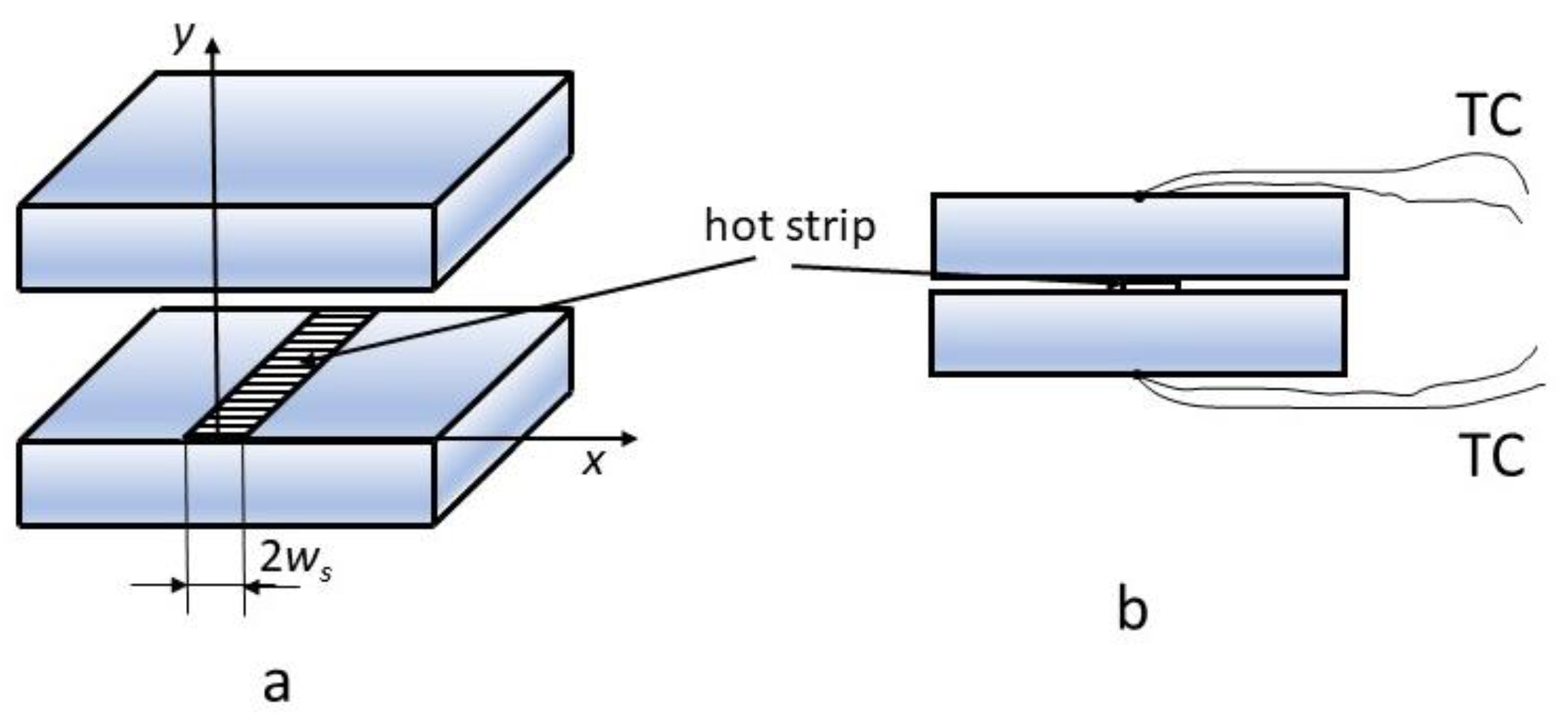
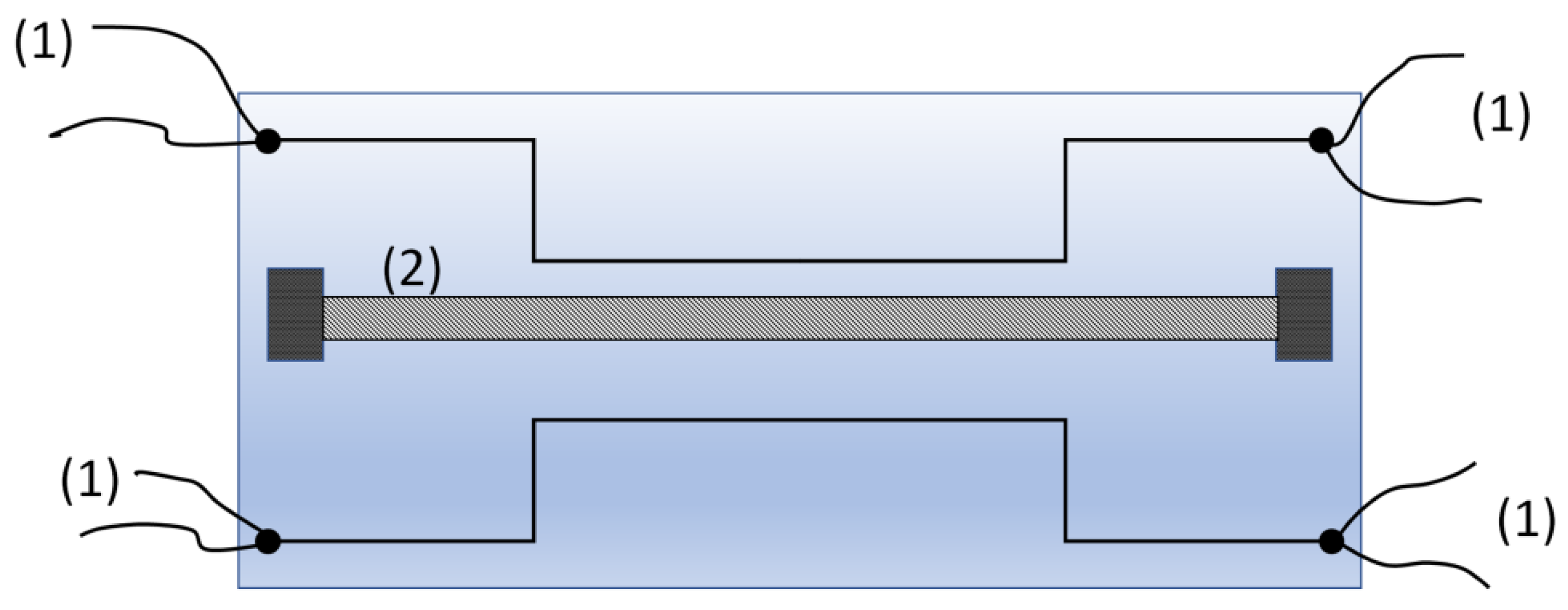
5.2. Transient Hot Strip

In the transient hot strip (THS) method [99,100], a metal strip, located between two slabs of the same material, is used both as a continuous plane heat source and a resistance thermometer (Figure 11).

To assure good thermal contact between the metal strip and the sample, a small amount of liquid can be introduced between the heater surfaces and the surfaces of the two specimens. Then, a constant current is supplied to the strip so that the applied heating power can be considered constant. Consequently, the strip temperature increases, depending on the thermal transport properties (thermal conductivity k and thermal diffusivity $\alpha$) of the material surrounding the heat source. The strip temperature increase also produces a rise in its electrical resistance. Thus, by measuring the strip temperature [101] or its electrical resistance [99] over a short period of time, it is possible to estimate k and $\alpha$. In particular, the temperature trend of the sensor is quasi-linear, and can be generally expressed as [101]:

$$\Delta T=A+Bf\left(\tau \right),$$

(18)

where the term A is related to the contact resistance at the interface between the strip and the sample material and the thermal capacity of the strip, the liquid (or glue) and the tested material, while $Bf\left(\tau \right)$ is a transient term mainly affected by the sample properties, above all, k. In detail, $B=B\left(\frac{\dot{Q}}{kL}\right)$, where $\dot{Q}$ is the heating power and L is the length of the strip; moreover, $f\left(\tau \right)$ is a complex dimensionless function of dimensionless time, i.e., the Fourier number $\tau =\sqrt{\alpha t/d^2}$ (d is the strip width). Finally, by evaluating the slope and the intercept of the regression line $\Delta T$ versus $f\left(\tau \right)$, the estimates of k and $\alpha$ are obtained, provided that the d of the strip is properly chosen [99].

Infinite sample geometry is usually assumed in this method. This assumption is valid only during the first part of the experiment, when the thermal field at the strip border is not affected by the sample surface boundary conditions. Therefore, homogeneous samples having medium or low thermal conductivities, and that are at least a couple of millimeters thick, are normally suitable for this experimental procedure. On the contrary, if the sample thickness is smaller or has a high thermal conductivity, the above assumptions are valid only for a very limited time range and, therefore, the experiment may not be realized if the laboratory equipment are not suited. In order to check the correctness of the assumed hypotheses, a thermocouple can be located at the sample border, and only data before its temperature increase are processed.

A modification of the sample geometry configuration to extend the nominal measurement time when testing high-conductivity ceramic bars has been suggested by Gustavsson et al. [101]. However, the THS method is not only suited for homogeneous solid materials, but also powdered materials [100], thermal insulation materials, such as organic foam [102] and aerogel [103], and liquids [104].

Gobbé et al. [105] combined the THW and THS methods to evaluate the thermal conductivity tensor of an orthotropic multilayer medium, in which each layer had isotropic thermal properties in the plane parallel to the layers. In particular, these authors used the THW method to measure planar thermal conductivity, while transient hot strip measurements together with an orthotropic model (in which the planar conductivity is used) yielded the conductivity in the transversal direction.

The reader can find a deep discussion about the uncertainty analysis of the THS method in [106]. Additionally, to reduce the uncertainty in the thermal diffusivity, Hammerschmidt [107] suggested the pulse hot strip method (PHS). This method combines the advantages of a strip heat source with temperature independent electric resistance and an accurate temperature measurement capability of a thin platinum wire. In fact, the used sensor consists of a strip made of manganin (heat source) and two wires of platinum working as a PRT (platinum resistance thermometer), which are both laminated between thin sheets of Kapton. Its scheme is shown in Figure 12.

Manganin has a very low temperature coefficient of resistance. Thus, the heat supplied to the sample is practically independent on temperature. On the contrary, platinum exhibits a meaningful change in electrical resistance with temperature; in fact, Pt wires are commonly used as PRTs (platinum resistance thermometers). The maximum of the pulse is taken as the starting signal. Then, this heat pulse traveling through the sample reaches the temperature sensors (wires) located at known distances r₁ and r₂ from the center of the strip. The thermal diffusivity is then obtained as a function of time t, as shown by Hammerschmidt [107]:

$$\alpha =\frac{r_2^2-r_1^2}{4t\ln \left(T_1/T_2\right)},$$

(19)

where T₁ and T₂ are the absolute temperatures measured by the two sensors distant r₁ and r₂ from the strip, respectively. In order to obtain greater accuracy and verify the assumed hypotheses, it is possible to determine $\alpha$ through the nonlinear regression of temperatures T₁ and T₂ versus time t by applying Equation (20)

$$T_1/T_2=\exp \left(\frac{{r_2}^2-{r_1}^2}{4\alpha t}\right),$$

(20)

and carrying out the nonlinear regression of T₁/T₂ data versus t, using $\alpha$ as the regression parameter. Such a procedure also allows one to verify whether the temperature trend agrees with the theory, and to evaluate the uncertainty of $\alpha$ through the covariance matrix of the unknowns [26].

Moreover, the PHS method has been extended for thermal effusivity measurements of drop-size liquids [108].

The evolution of THS to avoid its major drawback, due to the small temperature-dependent voltage, was suggested by Hammerschmidt and Mayer [109], and is known as transient hot bridge. This evolution foresees the use of a new sensor not affected by end effect (i.e., the temperature drop at the ends of the strip-shaped heater), which also minimizes the offset in the output voltage.

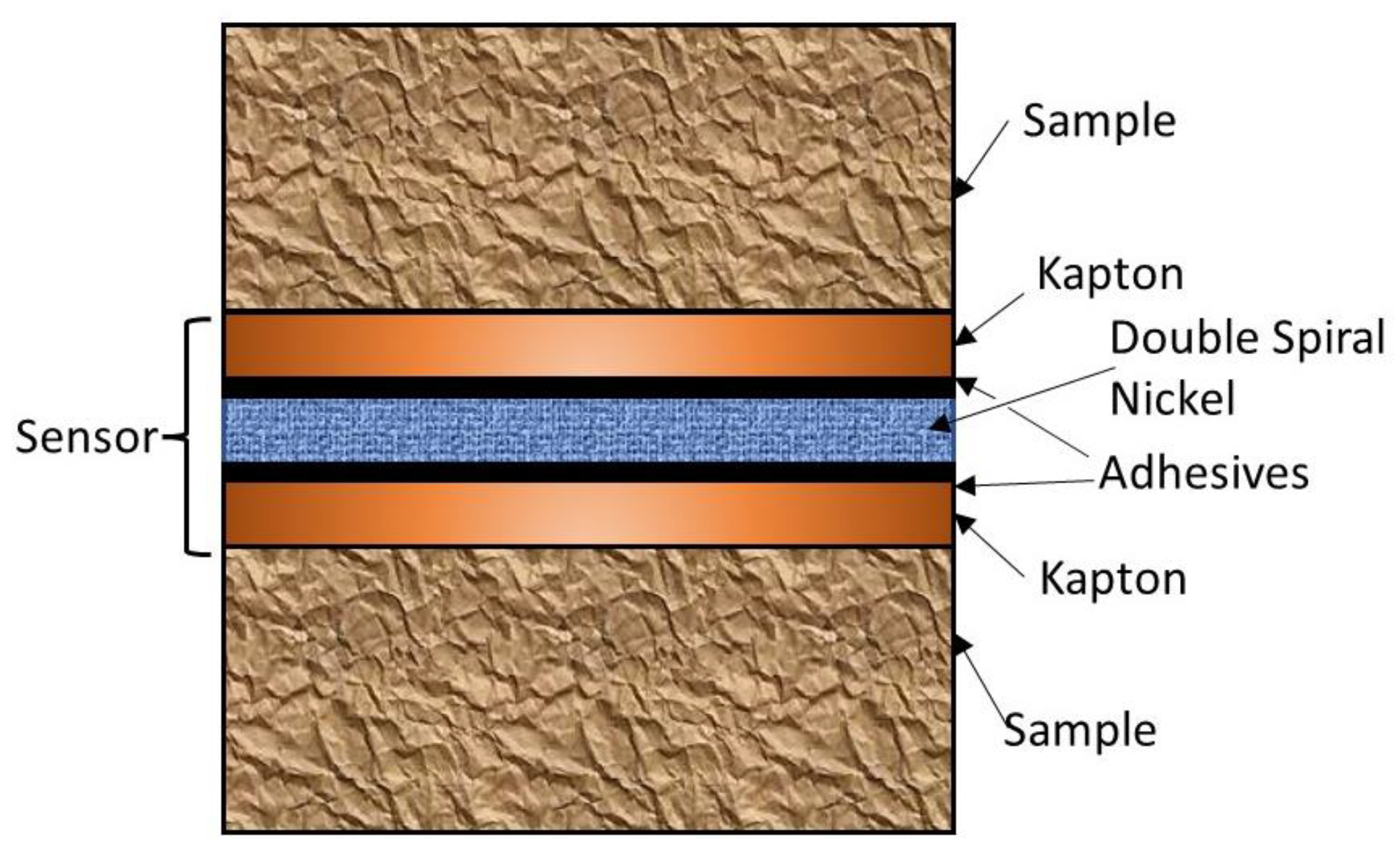
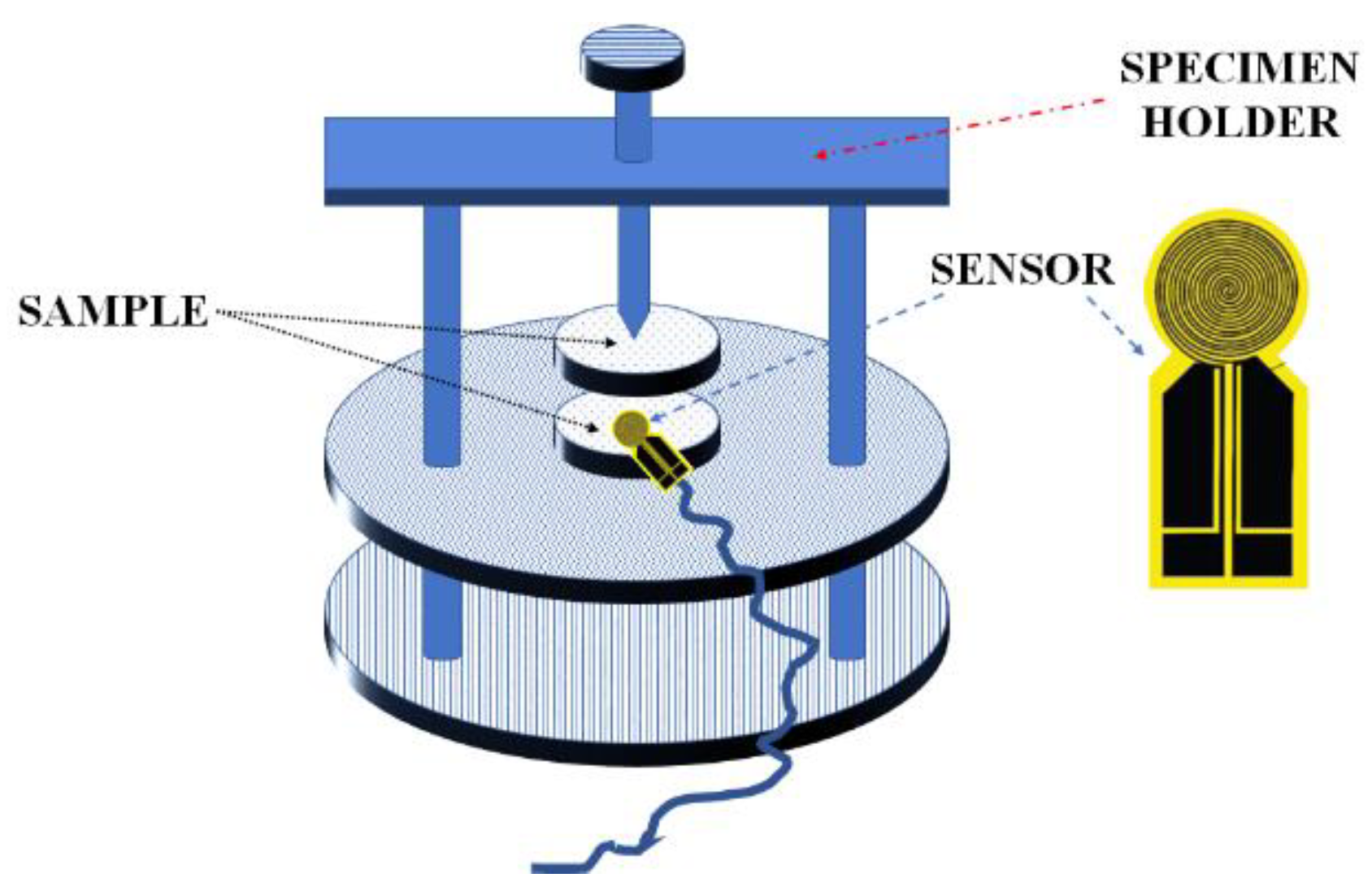
5.3. Transient Plane Source Method

The transient plane source (TPS) method was suggested by Gustafsson [110] to simultaneously estimate thermal conductivity and thermal diffusivity. Several advantages characterize the TPS method, such as the wide k range (from 0.005 to 500 W/m K) and the different kinds of materials suitable to be tested (solid, powder, liquid, or porous materials). It has also been applied to composite materials [111] and highly porous building materials [112]. Additionally, the sample can have different shapes (slab, thin film) [12,113].

This method uses a probe placed between two samples of the same material, forming a sandwich structure, as shown in Figure 13. It works both as a heat source and temperature sensor [113]. Additionally, the sensor usually consists of a double spiral (Figure 14) made of nickel and coated with a Kapton or mica insulation layer [12,113]. However, it can also be square-shaped [114].

The sensor is heated by an electric current flowing through it, and, consequently, its electrical resistance increases with temperature dependent on time. If the tested material is opaque under thermal radiation, the heat generated by the sensor is exclusively delivered to the sample by conduction. Then, the temperature increase in the sensor, $\Delta T$, can be split up into two parts:

$$\Delta T=\Delta T_i+\Delta T\left(\tau \right),$$

(21)

where $\Delta T_i$ is the temperature difference across the sensor insulation layer, which combines the effects of the thermal contact resistance and the adhesive between the heat element and the insulation layer of the sensor, and τ is the dimensionless time (Fourier number) defined as $\tau =\sqrt{\alpha t/r^2}$, with $\alpha$ representing the thermal diffusivity of the sample, and r the radius of the outermost ring of the sensor. $\Delta T\left(\tau \right)$ is the temperature rise in the sensor outer surface. In particular, when its double-spiral configuration is approximated by equally spaced concentric circular line sources, the term $\Delta T\left(\tau \right)$ is described by the following equation [113]

$$\Delta T\left(\tau \right)=\frac{\dot{Q}}{{\pi }^{3/2}rk}f\left(\tau \right).$$

(22)

$\dot{Q}$ is the heating power, k the thermal conductivity of the sample, and $f\left(\tau \right)$ is a dimensionless time function defined as

$$f\left(\tau \right)=\frac{1}{{\left[m\left(m+1\right)\right]}^2}{\displaystyle \underset{0}{\overset{\tau }{\int }}\frac{1}{{\sigma }^2}{\displaystyle \sum _{i=1}^{m}i{\displaystyle \sum _{j=1}^{m}j{e}^{-\frac{i^2+j^2}{4m^2{\sigma }^2}}{I}_0\left(\frac{ij}{2m^2{\sigma }^2}\right)}}d\sigma },$$

(23)

where m is the number of concentric rings and I₀ the modified zero-order Bessel function.

An expression similar to Equation (23) describes how the sensor resistance R changes [113]:

$$R\left(\tau \right)=R^{*}+\frac{\alpha R_0{P}_0}{{\pi }^{3/2}rk}f\left(\tau \right),$$

(24)

where $R^{*}=R_0\left(1+\alpha \Delta T_i\right)$ and R₀ is the initial resistance of the sensor. The electrical resistance of the sensor is recorded as a function of time.

In order to measure the thermal conductivity or the diffusivity of the sample, a linear least squares fitting procedure is applied to recorded data using Equation (23) or Equation (24).

Elkholy et al. [116] theoretically established a new procedure involving the TPS method coupled with the so-called dynamic plane source (DPS) method [117] to measure the thermal conductivity, diffusivity, and heat capacity of anisotropic materials. When testing such materials, Zhang et al. [118] showed that the sensor thickness affects the accuracy of the thermal conductivity measurements. This is particularly true for high thermal conductivity materials. To increase the accuracy, these authors suggested the use of sensors with larger radii. The influence of the sensor geometry on the accuracy of thermal conductivity measurements for low-conductivity materials has been investigated by Zheng et al. [119]. To improve the accuracy of the measurements, they defined some polynomial correction functions for commonly used sensors.

Recently, a new plane source method designed to measure thermal effusivity and conductivity using two experiments has been suggested by Malinaric and Elkholy [120].

5.4. Modeling Inverse Transient Techniques

5.4.1. One-Dimensional Models

One of the inverse transient techniques for thermal property estimation of solid materials, called the “plane source method”, requires an experimental apparatus consisting of a thin electrical heater sandwiched between two samples of the same material and thickness [121,122,123]. This apparatus is similar to the plane source method (Section 5.3), but data processing is mainly based on inverse problem technique. Using this experimental set-up, the thin heater warms up both the samples at the same rate. Additionally, all the external surfaces are insulated, and this feature makes the device suitable for thermal property measurements of high conductivity materials. A schematic of this setup is shown in Figure 15a, where $g\left(t\right)$ is the uniform volumetric heat generation within the heater. Note that the heater can be switched on either for the whole duration of the experiment t_N or for a shorter period (from t = 0 to t_h). Applying the heating in one of these two ways or the other is a matter of optimization (see Section 5.5).

As the boundary surfaces of the setup are all thermally insulated, the three-dimensional (3D) heat conduction problem reduces to one-dimension (1D). In addition, for the sake of thermal symmetry, the three-layer configuration (specimen–heater–specimen) reduces to the two-layer configuration depicted in Figure 15b. In this figure, the first layer represents one half of the heater and the other is the sample.

Non-embedded temperature sensors are used to measure the temperature at the front and the rear of the sample. Additionally, the parameter estimation procedure requires to minimize the least squares norm between the measured temperature values and the temperature computed through the model. For this purpose, the Gauss method can be used.

$${\underset{\_}{b}}^{\left(i+1\right)}={\underset{\_}{b}}^{\left(i\right)}+{\underset{\_}{P}}^{\left(i\right)}{\underset{\_}{X}}^{T\left(i\right)}\left[\underset{\_}{Y}-{\underset{\_}{T}}^{\left(i\right)}\right],$$

(25)

$${\underset{\_}{P}}^{\left(i\right)}={\left[{\underset{\_}{X}}^{T\left(i\right)}{\underset{\_}{X}}^{\left(i\right)}\right]}^{-1},$$

(26)

where i is the iteration index, $\underset{\_}{b}$ denotes the estimated parameter vector containing the thermal properties of the sample under investigation, $\underset{\_}{Y}$ is the measured temperature vector, $\underset{\_}{T}$ is the calculated temperature vector, and $\underset{\_}{X}$ is the sensitivity coefficient matrix [27].

Attention must be paid to the choice of thermal properties to be investigated, especially when dealing with mutually dependent properties, such as thermal conductivity k and diffusivity $\alpha$ = k/C, volumetric heat capacity C and $\alpha$, or k and thermal effusivity $\epsilon =\sqrt{kC}$. However, in all cases, sensitivity coefficients of temperature with respect to the properties of interest must be studied to verify whether a mutual dependence is present between parameters. In fact, to ensure the convergence of the iterative procedure given above, it is recommended to apply sensitivity coefficients that are large in magnitude and linearly independent [27,124]. Alternatively, the cross correlation coefficients between the parameters can be studied [26].

Furthermore, the parameter estimation procedure will be affected not only by the mutual dependence between properties and measurement errors, but also by other disturbances related to the experimental setup, such as the thermal capacity of the heater and the contact resistance at the sample–heater interface. Several approaches exist in the specialized literature to handle these uncertainty sources. The most common aim to experimentally reduce the heater thermal capacity using a very thin metallic heater, as well as the interface contact resistance through a suited thermal interface material [125]. Therefore, these disturbances are often neglected in the mathematical models commonly used in the specialized literature to compute the temperature response of the sample [27,126]. Specifically, a single layer (the sample) is assumed, subjected to a surface heat flux at the front side and insulated at the rear.

In the opposite direction, only a few authors have considered the effect of the thermal inertia of the heater; for instance, Dowding et al. [121] used a multilayer numerical model with known heater properties, and D’Alessandro and de Monte [122] suggested a single-layer analytical model with a fourth kind boundary condition applied to the heated surface of the sample. Specifically, this boundary condition occurs when a heat flux is supplied to a perfectly-conductive thin layer which is in perfect contact with a whatever domain. It is not very common in the literature, but is of great importance, as it allows a thin film to be modeled as a lumped body, thus maintaining its heat capacity [127]. It is worth noting that D’Alessandro and de Monte [122] reported that it is not possible to simultaneously estimate k and C of the sample and the heat capacity of the heater due to correlation between these parameters. However, the volumetric heat capacity of the heater can easily be measured with a calorimeter. Alternatively, an inverse technique can be used to estimate only the thermal properties of the heater when a sample of known properties is considered.

Furthermore, the non-negligible contact resistance can be included in the effective thermal conductivity of the heater [125]. Exceptions are the research papers authored by Bovesecchi and Coppa [128] and by D’Alessandro et al. [129], who used specific types of boundary conditions to account for the imperfect thermal contact.

Additionally, multilayer analytical models accounting for both perfect and imperfect thermal contact at the heater–sample interface are discussed in [130].

If the thin heater behaves as a lumped body, the heat conduction transient model involves a one-dimension (1D) single-layer rectangular body (sample) subjected to a sixth kind boundary condition [17,131] at the heated surface [132]. This boundary condition is similar to that of the fourth kind, but in such a case the thin layer is in imperfect contact with the domain in which heat conduction occurs. According to the authors of Ref. [132], the use of such a model not only allows the thermal properties of the sample (e.g., thermal conductivity k and volumetric heat capacity C) to be simultaneously estimated, but also allows the thermal contact resistance to be estimated with the same experiment when a heater of known properties is used. This possibility has been verified through simulated experiments using a random error generator [132].

Among the 1D models, an interesting approach was suggested by Monde et al. [133], aimed at obtaining measurements of thermal conductivity and diffusivity independent on the surface conditions of the samples. In fact, the required temperature measurements were given by sensors embedded in the specimens arranged in a three-layer device (not at the interface surfaces). These data were then used in an estimation procedure involving a 1D inverse solution of heat flux. The authors claimed an accuracy of the estimated parameters greater than 5%, despite the uncertainty due to the locations of the temperature sensors.

The stepwise transient (SWT) method suggested by Kubičár and Bohác [134] was used to measure thermal conductivity and diffusivity of low-conductivity materials. It involves a four-layer device (sample–heater–sample–sample) in which the specimen is cut into three pieces. Additionally, a plane heat source is placed at the first interface, while thermocouples are located at the other sample–sample interface. A fitting procedure is used to retrieve the unknown parameters, paying attention to the correlation among the evaluated parameters, as shown by the sensitivity coefficients of temperature with respect to these parameters. In fact, this procedure does not work properly when the parameters are highly correlated.

The effect of heat capacity and thermal conductivity of the heat source can be also considered, as shown by Malinarič and Dieška [135]. The pulse transient method [135] is a modification of the SWT method, in which the samples are warmed up over a finite heating time.

5.4.2. Multidimensional Models

Other methods require non-uniform space heating described by multidimensional models. For instance, Dowding et al. [136] applied stepwise uniform heating to a sample–heater–sample configuration (similar to that depicted in Figure 15a) to contemporarily estimate the directional thermal conductivities of a carbon–carbon composite as well as its volumetric heat capacity, using a heater of known properties appearing in a two-dimensional (2D) numerical model. Moreover, when the heater was neglected, D’Alessandro et al. investigated an analytical 2D model involving stepwise uniform heating, applied for a finite period of time, to simultaneously estimate the thermal conductivity and effusivity of isotropic high-conductivity materials [123].

Rodrigues et al. [137] investigated the possibility of estimating the directional thermal conductivities of three-dimensional orthotropic solids by applying partial heating on a single surface. They used simulated transient measurements containing random errors, and the Levenberg–Marquardt method to minimize the ordinary least squares norm.

The Levenberg–Marquardt algorithm was also used by Somasundharam and Reddy for the simultaneous estimation of the principal thermal conductivities and heat capacity of a unidirectional fiber-reinforced carbon composite [138]. Their experimental setup consisted of a planar electrical heater sandwiched between two identical samples, whose temperatures were non-intrusively measured with an IR camera. Additionally, the heat capacity of the heater and the contact resistance at the sample–heater interface were included in the mathematical model, numerically solved by means of the finite volume method.

El Rassy et al. [139] experimentally investigated the simultaneous estimation of thermal properties of an orthotropic composite sample using local excitation (a CO₂ laser beam) on the front surface. In this case, the identification procedure was based on the minimization of the least squares difference between the outputs of a 3D thermal quadrupoles model and the temperature measurements of the front surface recorded by an IR camera.

An interesting approach has been suggested by de Monte and Beck, which used a sinusoidal in space surface heat flux to determine thermal conductivities of orthotropic thin film placed on a substrate in time-independent conditions [140].

5.5. Optimum Experiment Design

In this section, the common criteria and the novel approaches suggested for optimal experiment design are discussed when dealing with parameter estimation problems.

One main principle in parameter estimation is that the measured temperatures must be sensitive to the parameters of interest [124,125]: the more sensitive the temperature is (i.e., the larger the sensitivity coefficient is), the more valid the temperature measurements are, that is, the highest possible level of insight and information must derive from the experiments. To reach this goal, the experimental apparatus should be properly designed.

Optimal experiment design provides the best conditions to take measurements, in order to obtain the greatest accuracy of the estimated parameters. These conditions concern the optimum location of the sensors, the optimum measurement time, the most suited boundary, and initial conditions. It also may suggest which quantities should be measured.

Several criteria defining the optimal experiments have been suggested in terms of the Fisher information matrix [141,142,143], which involves the ${\underset{\_}{X}}^T\underset{\_}{X}$ matrix (where $\underset{\_}{X}$ is the sensitivity matrix, that is, the matrix of the sensitivity coefficients). In particular, the Fisher matrix considers both the sensitivity coefficients of temperature with respect to the model parameters and the measurement uncertainties [144]. The most common optimization criteria, known as D-optimality criteria, are based on the maximization of the determinant of the Fisher matrix. These criteria are recommended as they minimize the confidence region of the estimated parameters when certain statistical assumptions are valid (see [27], Chap. 8 for an exhaustive discussion). In this study, Beck and Arnold suggested a specific D-optimum criterion, called the Δ⁺ criterion, involving the maximization of the dimensionless ${\underset{\_}{X}}^T\underset{\_}{X}$ determinant. The greater this determinant is, the lower the correlation between the parameters, thus one can more easily obtain the estimation procedure convergence. This optimization criterion was used by Taktak et al. [126] to decide both the experiment and heating times in the estimation of the thermal properties of carbon fiber–epoxy matrix composites. They demonstrated that applying a finite time heating increases the determinant value. More recently, D’Alessandro and de Monte [122] applied the Δ⁺ criterion to design the optimum experiment to simultaneously estimate thermal conductivity and volumetric heat capacity of metallic samples when using the plane heat source method, as discussed in Section 5.4.1. Additionally, using the same procedure, D’Alessandro and de Monte provided numerical correlations useful to define the optimum experiment and heating times for a plane-source-method-based experimental apparatus, taking into account the heat capacity of the heater and the contact resistance at the heater–sample interface [132].

Additionally, D’Alessandro et al. [123] applied the Δ⁺ criterion to find the optimal experiment conditions (uniform or partial heating) when thermal conductivity and effusivity of isotropic high-conductivity materials are simultaneously estimated. They concluded that the partial heating is not beneficial when testing isotropic materials.

Moreover, the application of this optimization procedure to different sensor configurations through the comparison of the Δ⁺ determinant values makes it possible to identify the best sensor location [123].

Another possible criterion is based on the minimization of the condition number related to the ${\underset{\_}{X}}^T\underset{\_}{X}$ matrix (this number is defined as the ratio between its largest and smallest eigenvalue) [145,146,147]: the closer this number is to one, the better-posed is the inverse problem. Even if it is so, no assurance exists that the variances of the parameters are reduced [148].

Mzali et al. showed that the best estimate of the thermal properties of orthotropic solids can be obtained through a compromise between a D-optimality criterion based on the maximization of the ${\underset{\_}{X}}^T\underset{\_}{X}$ determinant and the minimization of its condition number [146]. This compromise is obtained with the so-called E-optimality criterion, which uses the maximization of the minimum eigenvalue of the ${\underset{\_}{X}}^T\underset{\_}{X}$ matrix. Thus, the highest variance among the estimated parameters decreases, and all the normalized variances are more or less equal [148].

Moreover, it is also possible to adopt the A-optimality criterion, based on the minimization of the trace of the ${\left[{\underset{\_}{X}}^T\underset{\_}{X}\right]}^{-1}$ matrix (i.e., sum of its diagonal components). This trace is strictly related to the sum of the parameter variances [148].

In contrast to traditional optimality criteria, some researchers have also tried different approaches in optimal experiment design. For instance, Ruffio et al. [148] defined a “robust” design, with the goal of optimizing the thermocouple locations in a 2D sample of an orthotropic material. The location was less sensitive to the small changes of the first approximation of the unknown parameters. The authors based their optimum criterion on the maximum likelihood estimation procedure, combined with stochastic optimization algorithms, such as particle swarm optimization and evolution strategies.

Machine-learning-based approaches (such as Bayesian optimization, Monte Carlo tree search, neural network, Gaussian process regression) have also been suggested by Dieb and Tsuda, [149] and Wei et al. [150]. Recently, Gasparin et al. solved an optimization procedure based on a D-optimum criterion involving a convex relaxation strategy, in order to reduce the computational cost of the search of optimum sensor location for a 2D inverse problem [151].

6. Conclusions

The extremely relevant importance of the knowledge the thermophysical data of materials, when used in analyzing thermal device behavior or thermal phenomena, is outlined in the above-reported review. Among all the TP evaluation methods and measuring techniques described, the following results are best-suited for these applications:

–

Transient hot wire or thermal conductivity probe, for measuring thermal conductivity.

–

Differential thermal analysis or differential scanning calorimetry, for thermal capacitance.

–

Laser flash method, for thermal diffusivity of samples in the shape of slabs.

–

Dual-probe method, for thermal diffusivity in bulk samples.

The contemporary measurement of different quantities, e.g., thermal conductivity and thermal diffusivity, can be carried out by means of specialized techniques, such as transient hot strip and transient plane source methods. Additionally, other inverse techniques involving parameter estimation can provide a great help in simultaneously determining the TP from the recorded temperature values; however, care must be taken in the experiment design and in data processing to avoid mutual correlation between the evaluated properties.

Additionally, some unique applications of the described methods, and the actions devoted to minimize the measurement problems met, are reported in the list of the above-mentioned cases.

References

1. Bud, R.; Warner, D.J. Instruments of Science; Routledge: New York, NY, USA, 1998; pp. 170–171. ISBN 9780815315612. [Google Scholar]
2. Höhne, G.; Hemminger, W.F.; Flammersheim, H.J. Differential Scanning Calorimetry; Springer: Heidelberg/Berlin, Germany, 2003; ISBN 978-3-540-00467-7. [Google Scholar]
3. Corsan, J.M. Axial heat flow methods of thermal conductivity measurement for good conducting materials. In Compendium of Thermophysical Property Measurement Methods: Recommended Measuring Techniques and Practices; Maglić, K.D., Cezairliyan, A., Peletsky, V.E., Eds.; Springer: Boston, MA, USA, 1992; Volume 2, pp. 3–31. [Google Scholar]
4. Wang, Q.; Dai, J.M.; Coppa, P. Thermophysical property measurement of thermal protective material by guarded plane source method. J. Tianjin Univ. Sci. Technol. 2010, 43, 1086–1092. [Google Scholar]
5. Flynn, D.R. Thermal conductivity of loose-fill materials by a radial-heat-flow method. In Compendium of Thermophysical Property Measurement Methods: Recommended Measuring Techniques and Practices; Maglić, K.D., Cezairliyan, A., Peletsky, V.E., Eds.; Springer: Boston, MA, USA, 1992; Volume 2, pp. 33–75. [Google Scholar]
6. De Ponte, F.; Langlais, C.; Klarsfeld, S. Reference guarded hot plate apparatus for the determination of steady-state thermal transmission properties. In Compendium of Thermophysical Property Measurement Methods: Recommended Measuring Techniques and Practices; Maglić, K.D., Cezairliyan, A., Peletsky, V.E., Eds.; Springer: Boston, MA, USA, 1992; Volume 2, pp. 99–131. [Google Scholar]
7. Healy, J.J.; de Groot, J.J.; Kestin, J. The theory of the transient hot-wire method for measuring thermal conductivity. Physica B+C 1976, 82, 392–408. [Google Scholar] [CrossRef]
8. Hong, S.W.; Kang, Y.T.; Kleinstreuer, C.; Koo, J. Impact analysis of natural convection on thermal conductivity measurements of nanofluids using the transient hot-wire method. Int. J. Heat Mass Transf. 2011, 54, 3448–3456. [Google Scholar] [CrossRef]
9. Turgut, A.; Sauter, C.; Chirtoc, M.; Henry, J.F.; Tavman, S.; Tavman, I.; Pelzl, J. AC hot wire measurement of thermophysical properties of nanofluids with 3ω method. Eur. Phys. J. Spec. Top. 2008, 153, 349–352. [Google Scholar] [CrossRef]
10. Yoo, D.; Lee, J.; Lee, B.; Kwon, S.; Koo, J. Further elucidation of nanofluid thermal conductivity measurement using a transient hot-wire method apparatus. Heat Mass Transf. 2018, 54, 415–424. [Google Scholar] [CrossRef]
11. Lee, J.; Lee, H.; Baik, Y.J.; Koo, J. Quantitative analyses of factors affecting thermal conductivity of nanofluids using an improved transient hot-wire method apparatus. Int. J. Heat Mass Transf. 2015, 89, 116–123. [Google Scholar] [CrossRef]
12. Ahadi, M.; Andisheh-Tadbir, M.; Tam, M.; Bahrami, M. An improved transient plane source method for measuring thermal conductivity of thin films: Deconvoluting thermal contact resistance. Int. J. Heat Mass Transf. 2016, 96, 371–380. [Google Scholar] [CrossRef]
13. Wechsler, A.E. The probe method for measuring thermal conductivity. In Compendium of Thermophysical Property Measurement Methods: Recommended Measuring Techniques and Practices; Maglić, K.D., Cezairliyan, A., Peletsky, V.E., Eds.; Springer: Boston, MA, USA, 1992; Volume 2, pp. 161–185. [Google Scholar]
14. Gross, U.; Tran, L.T.S. Radiation effects on transient hot-wire measurements in absorbing and emitting porous media. Int. J. Heat Mass Transf. 2004, 47, 3279–3290. [Google Scholar] [CrossRef]
15. Coquard, R.; Baillis, D.; Quenard, D. Experimental and theoretical study of the hot-wire method applied to low-density thermal insulators. Int. J. Heat Mass Transf. 2006, 49, 4511–4524. [Google Scholar] [CrossRef]
16. Castán-Fernández, C.; Marcos-Robredo, G.; Ángel Rey-Ronco, M.; Alonso-Sánchez, T. Design, construction and commissioning of an apparatus for measuring the thermal conductivity of geothermal grouting materials based on the transient hot wire method. Proceedings 2018, 2, 1496. [Google Scholar]
17. Carlslaw, H.S.; Jaeger, J.C. Conduction of Heat in Solids; Oxford Univ. Press: London, UK, 1959. [Google Scholar]
18. Bovesecchi, G.; Coppa, P.; Pistacchio, S. A new thermal conductivity probe for high temperature tests for the characterization of molten salts. Rev. Sci. Instrum. 2018, 89, 055107. [Google Scholar] [CrossRef] [PubMed]
19. Fukuyama, H.; Yoshimura, T.; Yasuda, H.; Ohta, H. Thermal conductivity measurements of liquid mercury and gallium by a transient hot wire method in a static magnetic field. Int. J. Thermophys. 2006, 27, 1760–1777. [Google Scholar] [CrossRef]
20. Coppa, P.; Pasquali, G. Thermal conductivity of lipidic emulsions and its use for production and quality control. In Proceedings of the 2nd International Symposium on Instrumentation Science and Technology, Jinan, China, 18–22 August 2002. [Google Scholar]
21. Hopper, F.C.; Lepper, F.R. Transient heat flow apparatus for determination of thermal conductivities. ASHVE Trans. 1950, 56, 309. [Google Scholar]
22. Zhang, Y.P.; Liang, X.G.; Wang, Z.; Ge, X.S. A method of determining the thermophysical properties and calorific intensity of the organ or tissue of a living body. Int. J. Thermophys. 2000, 21, 207–215. [Google Scholar] [CrossRef]
23. Parker, W.J.; Jenkins, R.J.; Butler, C.P.; Abbot, G.L. Flash method of determining thermal diffusivity heat capacity and thermal conductivity. J. App. Phys. 1961, 32, 1679–1684. [Google Scholar] [CrossRef]
24. Maillet, D.; Moyne, C.; Remy, B. Effect of a thin layer on the measurement of the thermal diffusivity of a material by a flash method. Int. J. Heat Mass Transf. 2000, 43, 4057–4060. [Google Scholar] [CrossRef]
25. Matteis, P.; Campagnoli, E.; Firrao, D.; Ruscica, G. Thermal diffusivity measurements of metastable austenite during continuous cooling. Int. J. Therm. Sci. 2008, 47, 695–708. [Google Scholar] [CrossRef] [Green Version]
26. Brandt, S. Statistical and Computational Methods in Data Analysis; North Holland Pub: Amsterdam, The Netherlands, 1970. [Google Scholar]
27. Beck, J.V.; Arnold, K.J. Parameter Estimation in Engineering and Science; Wiley: New York, NY, USA, 1977. [Google Scholar]
28. Thermitus, M.A.; Laurent, M. New logarithmic technique in the flash method. Int. J. Heat Mass Transf. 1977, 40, 4183–4190. [Google Scholar] [CrossRef]
29. Milosevic, N.; Raynaud, M.; Maglic, K. Estimation of thermal contact resistance between the materials of double-layer sample using the laser flash method. Inverse Probl. Eng. 2002, 10, 85–103. [Google Scholar] [CrossRef]
30. Potenza, M.; Cataldo, A.; Bovesecchi, G.; Corasaniti, S.; Coppa, P.; Bellucci, S. Graphene nanoplatelets: Thermal diffusivity and thermal conductivity by the flash method. AIP Adv. 2017, 7, 075214. [Google Scholar] [CrossRef] [Green Version]
31. Taylor, R.E. Thermal-property and contact-conductance measurements of coatings and thin films. Int. J. Thermophys. 1998, 19, 931–939. [Google Scholar] [CrossRef]
32. Bocchini, G.F.; Bovesecchi, G.; Coppa, P.; Corasaniti, S.; Montanari, R.; Varone, A. Thermal diffusivity of sintered steels with flash method at ambient temperature. Int. J. Thermophys. 2016, 37. [Google Scholar] [CrossRef]
33. Li, N.; Wang, Y.; Liu, Q.; Peng, H. Evaluation of thermal-physical properties of novel multicomponent molten nitrate salts for heat transfer and storage. Energies 2022, 15, 6591. [Google Scholar] [CrossRef]
34. Bison, P.; Cernuschi, F.; Grinzato, E. Ageing evaluation of thermal barrier coating: Comparison between pulsed thermography and thermal wave interferometry. Quant. InfraRed Thermogr. J. 2006, 3, 169–181. [Google Scholar] [CrossRef] [Green Version]
35. Cape, J.A.; Lehman, G.W. Temperature and finite pulse time effects in the flash method for measuring thermal diffusivity. J. Appl. Phys. 1963, 34, 1909. [Google Scholar] [CrossRef]
36. Bellucci, S.; Bovesecchi, G.; Cataldo, A.; Coppa, P.; Corasaniti, S.; Potenza, M. Transmittance and reflectance effects during thermal diffusivity measurements of GNP samples with the flash method. Materials 2019, 12, 696. [Google Scholar] [CrossRef] [Green Version]
37. Potenza, M.; Coppa, P.; Corasaniti, S.; Bovesecchi, G. Numerical simulation of thermal diffusivity measurements with the laser-flash method to evaluate the effective property of composite materials. J. Heat Transf. (ASME) 2021, 143, 072102. [Google Scholar] [CrossRef]
38. Bison, P.; Cernuschi, F.; Capelli, S. A thermographic technique for the simultaneous estimation of in-plane and in-depth thermal diffusivities of TBCs. Surf. Coat. Technol. 2011, 205, 3128–3133. [Google Scholar] [CrossRef]
39. Azumi, T.; Takahashi, Y. Novel finite pulse-width correction in flash thermal diffusivity measurement. Rev. Sci. Instrum. 1981, 52, 1411–1413. [Google Scholar] [CrossRef]
40. dell’Avvocato, G.; Palumbo, D.; Palmieri, M.E.; Galietti, G. Evaluation of effectiveness of heat treatments in boron steel by laser thermography. Eng. Proc. 2021, 8, 8. [Google Scholar]
41. Sfarra, S.; Cicone, A.; Yousefi, B.; Perilli, S.; Robol, L.; Maldague, X.P.V. Maximizing the detection of thermal imprints in civil engineering composites via numerical and thermographic results pre-processed by a groundbreaking mathematical approach. Int. J. Therm. Sci. 2022, 177, 107553. [Google Scholar] [CrossRef]
42. Pawar, S.S.; Vavilov, V.P. A novel one-sided diffusivity evaluation technique versus Parker’s method in application to carbon/epoxy composite. In Proceedings of the 12th International Conference on Quantitative Infrared Thermography (QIRT 2015), Mahabalipuram, India, 6–10 July 2015. [Google Scholar]
43. Heckman, R.C. Finite pulse-time and heat-loss effects in pulse thermal diffusivity measurements. J. Appl. Phys. 1973, 44, 1465–1470. [Google Scholar] [CrossRef]
44. Clark, L.M., III; Taylor, R.E. Radiation loss in the flash method for thermal diffusivity. J. Appl. Phys. 1975, 46, 714–719. [Google Scholar] [CrossRef]
45. Degiovanni, A. Diffusivité et méthode flash. Rev. Gén. Therm. 1977, 185, 420–442. [Google Scholar]
46. Balageas, D.L. Nouvelle méthode d’interprétation des thermogrammes pour la détermination de la diffusivité thermique par la méthode impulsionnelle (méthode flash). Rev. Phys. Appl. 1982, 17, 227–237. [Google Scholar] [CrossRef]
47. Degiovanni, A.; Laurent, M. Une nouvelle technique d’identification de la diffusivité thermique pour la méthode “flash”. Rev. Phys. Appl. 1986, 21, 229–237. [Google Scholar] [CrossRef] [Green Version]
48. Pech-May, N.W.; Mendioroz, A.; Agustín Salazar, A. Generalizing the flash technique in the front-face configuration to measure the thermal diffusivity of semitransparent solids. Rev. Sci. Instrum. 2014, 85, 104902. [Google Scholar] [CrossRef]
49. Salazar, A.; Mendioroz, A.; Apiñaniz, E.; Pradere, C.; Noël, F.; Batsale, J.-C. Extending the flash method to measure the thermal diffusivity of semitransparent solids. Meas. Sci. Technol. 2014, 25, 035604. [Google Scholar] [CrossRef]
50. Bison, P.; Grinzato, E.; Marinetti, S. Local thermal diffusivity measurement. Quant. InfraRed Thermogr. J. 2004, 1, 241–250. [Google Scholar] [CrossRef]
51. Hay, B.; Filtz, J.R.; Hameury, J.; Rongione, L. Uncertainty of thermal diffusivity measurements by laser flash method. Int. J. Thermophys. 2005, 26, 1883. [Google Scholar] [CrossRef]
52. Bison, P.; Ferrarini, G.; Glorieux, C. Pulsed thermography in the assessment of in-plane thermal diffusivity: Aperiodic, periodic and random patterns. In Proceedings of the ICPPP21—International Conference on Photoacoustic and Photothermal Phenomena, Bled, Slovenia, 19–24 June 2022. [Google Scholar]
53. Cernuschi, F.; Russo, A.; Lorenzoni, L.; Figari, A. In-plane thermal diffusivity evaluation by infrared thermography. Rev. Sci. Instrum. 2001, 72, 3988–3995. [Google Scholar] [CrossRef]
54. Kalogiannakis, G.; Van Hemelrijck, D.; Longuemart, S.; Ravi, J.; Okasha, A.; Glorieux, C. Thermal characterization of anisotropic media in photothermal point, line, and grating configuration. J. Appl. Phys. 2006, 100, 063521. [Google Scholar] [CrossRef]
55. Krapez, J.C. Diffusivity measurement by using a grid-like mask. In Proceedings of the Journée SFT “Thermographie Infrarouge”, Chatillon, France, 31 March 1999. [Google Scholar]
56. Batsale, J.-C.; Battaglia, J.-L.; Fudym, O. Autoregressive algorithms and spatially random flash excitation for 2D non-destructive evaluation with infrared cameras. Quant. InfraRed Thermogr. J. 2004, 1, 5–20. [Google Scholar] [CrossRef]
57. Duquesne, L.; Lorrette, C.; Pradère, C.; Vignoles, G.L.; Batsale, J.-C. A flash characterization method for thin cylindrical multilayered composites based on the combined front and rear faces thermograms. Quant. Infrared Thermogr. J. 2016, 13, 182–194. [Google Scholar] [CrossRef] [Green Version]
58. Legaie, D.; Pron, H.; Bissieux, C. Resolution of an inverse heat conduction problem with a non-linear least square method in the Hankel space. Application to photothermal infrared thermography. J. Phys. Conf. Ser. 2008, 135, 012061. [Google Scholar] [CrossRef]
59. Chudzik, S. Thermal diffusivity measurement of insulating material using infrared thermography. Opto-Electron. Rev. 2011, 20, 40–46. [Google Scholar] [CrossRef]
60. Wrobel, G.; Rdzawski, Z.; Muzia, G.; Pawlak, S. Determination of thermal diffusivity of carbon/epoxy composites with different fiber content using transient thermography. J. Achiev. Mater. Manuf. Eng. 2009, 37, 518–525. [Google Scholar]
61. Bristow, K.L.; Kluitenberg, G.J.; Horton, R. Measurement of soil thermal properties with a dual-probe heat-pulse technique. Soil Sci. Soc. Am. J. 1994, 58, 1288–1294. [Google Scholar] [CrossRef]
62. Lubimova, H.A.; Lusova, L.M.; Firsov, F.V.; Starikova, G.N.; Shushpanov, A.P. Determination of surface heat flow. Maz. Ann. Geophys. 1961, 14, 157–167. [Google Scholar]
63. Jaeger, J.C. Application of the theory of heat conduction to geothermal measurements. In Terrestrial Heat Flow, Geophysical Monograph Series; Lee, W.H.K., Ed.; American Geophysical Union: Washington, DC, USA, 1965; Volume 8, pp. 7–23. [Google Scholar]
64. Campbell, G.S.; Calissendorff, K.; Williams, J.H. Probe for measuring soil specific heat using a heat pulse method. Soil Sci. Soc. Am. J. 1991, 55, 291–293. [Google Scholar] [CrossRef] [Green Version]
65. Bovesecchi, G.; Coppa, P.; Corasaniti, S.; Potenza, M. Critical analysis of dual-probe heat-pulse technique applied to measuring thermal diffusivity. Int. J. Thermophys. 2018, 39, 82. [Google Scholar] [CrossRef]
66. Bittle, R.R.; Taylor, R.E. Step-heating technique for thermal diffusivity measurements of large-grained heterogeneous materials. J. Am. Ceram. Soc. 1984, 67, 186–190. [Google Scholar] [CrossRef]
67. Vozar, L.; Sramkova, T. Two data reduction methods for evaluating of thermal diffusivity from step-heating measurements. Int. J. Heat Mass Transf. 1997, 40, 1647–1655. [Google Scholar] [CrossRef]
68. Griesinger, A.; Hurler, W.; Pietralla, M. A photothermal method with step heating for measuring the thermal diffusivity of anisotropic solids. Int. J. Heat Mass Transf. 1997, 40, 3049–3058. [Google Scholar] [CrossRef]
69. Albouchi, F.; Fetoui, M.; Rigollet, F.; Sassi, M.; Nasrallah, S.B. Optimal design and measurement of the effective thermal conductivity of a powder using a crenel heating excitation. Int. J. Therm. Sci. 2005, 44, 1090–1097. [Google Scholar] [CrossRef]
70. Bennis, G.L.; Vyas, R.; Gupta, R.; Ang, S.; Brown, W.D. Thermal diffusivity measurement of solid materials by the pulsed photothermal displacement technique. J. Appl. Phys. 1998, 84, 3602–3610. [Google Scholar] [CrossRef]
71. Olmstead, M.A.; Amer, N.M.; Kohn, S.; Fournier, D.; Boccara, A.C. Photothermal displacement spectroscopy: An optical probe for solids and surfaces. Appl. Phys. A 1983, 32, 141–154. [Google Scholar] [CrossRef]
72. Karner, C.; Mandel, A.; Trager, F. Pulsed laser photothermal displacement spectroscopy for surface studies. Appl. Phys. A 1985, 38, 19–21. [Google Scholar] [CrossRef]
73. Elperin, T.; Rudin, G. Theory of photothermal displacement method for determining physical properties of multilayered coatings. Int. J. Thermophys. 2009, 30, 1598–1615. [Google Scholar] [CrossRef]
74. Lopez-Baeza, E.; de la Rubia, J.; Goldsmid, H. Angstrom’s thermal diffusivity method for short samples. J. Phys. D Appl. Phys. 1987, 20, 1156. [Google Scholar] [CrossRef]
75. Vargas, H.; Miranda, L.C. Photoacoustic effect and related photothermal techniques. Phys. Rep. 1988, 161, 43–101. [Google Scholar] [CrossRef]
76. Tam, A.C. Applications of photoacoustic techniques. Rev. Mod. Phys. 1986, 58, 381–431. [Google Scholar] [CrossRef]
77. Almond, D.P.; Patel, P.M. Photothermal Sciences and Techniques; Chapman & Hall: London, UK, 1996. [Google Scholar]
78. Mercuri, F.; Marinelli, M.; Paoloni, S.; Zammit, U.; Scudieri, F. Latent heat investigation by photopyroelectric calorimetry. Appl. Phys. Lett. 2008, 92, 251911. [Google Scholar] [CrossRef]
79. Corasaniti, S.; Potenza, M.; Coppa, P.; Bovesecchi, G. Comparison of different approaches to evaluate the equivalent thermal diffusivity of building walls under dynamic conditions. Int. J. Thermal Sci. 2020, 150, 106232. [Google Scholar] [CrossRef]
80. Mercuri, F.; Paoloni, S.; Zammit, U.; Marinelli, M. Dynamics at the nematic-isotropic phase transition in aerosil dispersed liquid crystal. Phys. Rev. Lett. 2005, 94, 247801. [Google Scholar] [CrossRef]
81. Marinelli, M.; Mercuri, F.; Paoloni, S.; Zammit, U. Dynamics of nematic liquid crystal with quenched disorder in the random dilution and random field regimes. Phys. Rev. Lett. 2005, 95, 237801. [Google Scholar] [CrossRef] [PubMed]
82. Luc, A.M.; Balageas, D.L. Non-stationary thermal behavior of reinforced composites—A better evaluation of wall energy balance for convective conditions. In Proceedings of the 1st International Joint Conferences on Thermophysical Properties, Gaithersburg, MD, USA, 15–18 June 1981. [Google Scholar]
83. Luc-Bouhali, A.M.; Pujolà, R.M.; Balageas, D.L. Thermal diffusivity in situ measurements of carbon/carbon composite reinforcements. In Thermal Conductivity; Ashworth, T., Smith, D.R., Eds.; Plenum: London, UK, 1984; Volume 18, pp. 613–624. [Google Scholar]
84. Pujolà, R.M.; Balageas, D.L. Derniers développements de la méthode flash adaptée aux matériaux composites à renforcement orienté. High Temp.-High Press. 1985, 17, 623–632. (In French) [Google Scholar]
85. Bardon, J.-P.; Balageas, D.; Degiovanni, A.; Vuiiliermes, J. Thermics of composites and interfaces: Current status and perspectives. La Rech. Aérosp. 1989, 6, 37–45. [Google Scholar]
86. Balageas, D.; Déom, A.; Boscher, D. Composite thermal properties measurements by pulse photothermal radiometry. In Proceedings of the Eurotherm IV Conference Thermal Transfer in Composite Materials and Solid-Solid Interface, Nancy, France, 28 June–1 July 1988. [Google Scholar]
87. da Fonseca, H.M.; Barreto Orlande, H.R.; Fudym, O.; Sepúlveda, F. A statistical inversion approach for local thermal diffusivity and heat flux simultaneous estimation. Quant. Infrared Thermogr. J. 2014, 11, 170–189. [Google Scholar] [CrossRef]
88. Wawrzynek, A.; Nowak, A.J.; Bartoszek, M.; Delpak, R.; Hu, C.W. Theoretical analysis of applying thermography and inverse solutions to determine thermal properties of cementitious materials. Inverse Probl. Sci. Eng. 2005, 13, 23–46. [Google Scholar] [CrossRef]
89. Vavilov, V.; Burleigh, D.; Shiryaev, V. IR thermographic evaluation of thermal diffusivity anisotropy: Comparative analysis of some algorithms. Quant. InfraRed Thermogr. J. 2007, 4, 187–200. [Google Scholar] [CrossRef]
90. Malheiros, F.A.; Figueiredo, A.A.A.; da S. Ignacio, L.H.; Fernandes, H.C. Estimation of thermal properties using only one surface by means of infrared thermography. Appl. Therm. Eng. 2019, 157, 113696. [Google Scholar] [CrossRef]
91. Chaffar, K.; Chauchois, A.; Defer, D.; Zalewski, L. Thermal characterization of homogeneous walls using inverse method. Energy Build. 2014, 78, 248–255. [Google Scholar] [CrossRef]
92. Halloua, H.; Obbadi, A.; Errami, Y.; Sahnoun, S.; Elhassnaoui, A. Nondestructive inverse approach for determinign thermal and geometrical properties of internal defects in CFRP composites by lock-in thermography. In Proceedings of the 2016 International Conference on Electrical Sciences and Technologies in Maghreb (CISTEM), Marrakesh, Morocco, 26–28 October 2016. [Google Scholar]
93. Krankenhagen, R.; Jonietz, F.; Zirker, S. Determination of thermal parameters of concrete by active thermographic measurements. J. Nondestruct. Eval. 2022, 41, 25. [Google Scholar] [CrossRef]
94. Kooshki, S.; Mandelis, A.; Khodadad, M.; Khosravifard, A.; Melnikov, A. Determination of thermophysical properties and density volume fractions of Al2O3/Y-ZrO2 layered composite materials using transient thermography and two-stage inverse nonlinear heat conduction analysis. J. Appl. Phys. 2020, 127, 045110. [Google Scholar] [CrossRef]
95. Florez-Ospina, J.F.; Ospina-Borras, J.E.; Benitez-Restrepo, H.D. Non-destructive infrared evaluation of thermo-physical parameters in bamboo specimens. Appl. Sci. 2017, 7, 1253. [Google Scholar] [CrossRef] [Green Version]
96. Pavlov, T.R.; Staicu, D.; Vlahovic, L.; Konings, R.J.M.; van Uffelen, P.; Wenman, M.R. A new method for the characterization of temperature-dependent thermo-physical properties. Int. J. Therm. Sci. 2018, 124, 98–109. [Google Scholar] [CrossRef]
97. Groz, M.M.; Sommier, A.; Abisset-Chavanne, E.; Batsale, J.-C.; Pradere, C. Flash method and Bayesian inference for measurement of thermophysical fields. AIP Adv. 2021, 11, 105009. [Google Scholar] [CrossRef]
98. Pech-May, N.W.; Cifuentes, A.; Mendioroz, A.; Oleaga, A.; Salazar, A. Simultaneous measurement of thermal diffusivity and effusivity of solids using the flash technique in the front-face configuration. Meas. Sci. Technol. 2015, 26, 085017. [Google Scholar] [CrossRef]
99. Gustafsson, S.E.; Karawacki, E.; Khan, M.N. Transient hot-strip method for simultaneously measuring thermal conductivity and thermal diffusivity of solids and fluids. J. Phys. D Appl. Phys. 1979, 12, 1411–1421. [Google Scholar] [CrossRef]
100. Singh, R.; Saxena, N.S.; Chaudhary, D.R. Simultaneously measurement of thermal conductivity and thermal diffusivity of some building materials using the transient hot strip method. J. Phys. D Appl. Phys. 1985, 18, 1–8. [Google Scholar] [CrossRef]
101. Gustavsson, M.; Wang, H.; Trejo, R.M.; Lara-Curzio, E. On the use of the transient hot-strip method for measuring the thermal conductivity of high-conductivity thin bars. Int. J. Thermophys. 2006, 27, 1816–1825. [Google Scholar] [CrossRef]
102. Hu, R.; Ma, A.; Li, Y. Transient hot strip measures thermal conductivity of organic foam thermal insulation materials. Exp. Therm. Fluid Sci. 2018, 91, 443–450. [Google Scholar] [CrossRef]
103. Wei, G.; Zhang, X.; Yu, F. Thermal conductivity measurements on xonotlite-type calcium silicate by the transient hot-strip method. J. Univ. Sci. Technol. Beijing Miner. Metall. Mater. 2008, 15, 791–795. [Google Scholar] [CrossRef]
104. Lourenco, M.J.; Rosa, S.C.S.; Nieto de Castro, C.A.; Albuquerque, C.; Erdmann, B.; Lang, J.; Roitzsch, R. Simulation of the transient heating in an unsymmetrical, coated, hot-strip sensor with a self-adaptive finite-element method (SAFEM). Int. J. Thermophys. 2000, 21, 377–384. [Google Scholar] [CrossRef]
105. Gobbé, C.; Iserna, S.; Ladevie, B. Hot strip method: Application to thermal characterization of orthotropic media. Int. J. Therm. Sci. 2004, 43, 951–958. [Google Scholar] [CrossRef]
106. Hammerschmidt, U.; Sabuga, W. Transient Hot Strip (THS) Method: Uncertainty Assessment. Int. J. Thermophys. 2000, 21, 217–248. [Google Scholar] [CrossRef]
107. Hammerschmidt, U. A new pulse hot strip sensor for measuring thermal conductivity and thermal diffusivity of solids. Int. J. Thermophys. 2003, 24, 675–682. [Google Scholar] [CrossRef]
108. Gustavsson, M.; Nagai, H.; Okutani, T. Measurements of the thermal effusivity of a drop-size liquid using the pulse transient hot-strip technique. Int. J. Thermophys. 2005, 26, 1803–1813. [Google Scholar] [CrossRef]
109. Hammerschmidt, U.; Mayer, V. New transient hot-bridge sensor to measure thermal conductivity, thermal diffusivity, and volumetric specific heat. Int. J. Thermophys. 2006, 27, 840–865. [Google Scholar] [CrossRef]
110. Gustafsson, S.E. Transient plane source techniques for thermal conductivity and thermal diffusivity measurements of solid materials. Rev. Sci. Instrum. 1991, 62, 797–804. [Google Scholar] [CrossRef]
111. Kalaprasad, G.; Pradeep, P.; Mathew, G.; Pavithran, C.; Thomas, S. Thermal conductivity and thermal diffusivity analyses of low-density polyethylene composites reinforced with sisal, glass and intimately sisal/glass fibres. Compos. Sci. Technol. 2000, 60, 2967–2977. [Google Scholar] [CrossRef]
112. Bouguerra, A.; Ait-Mokhtar, A.; Amiri, O.; Diop, M.B. Measurement of thermal conductivity, thermal diffusivity and heat capacity of highly porous building materials using transient plane source technique. Int. Commun. Heat Mass Transf. 2001, 28, 1065–1078. [Google Scholar] [CrossRef]
113. Zhang, H.; Li, Y.; Tao, W. Effect of radiative heat transfer on determining thermal conductivity of semi-transparent materials using transient plane source method. Appl. Therm. Eng. 2017, 114, 337–345. [Google Scholar] [CrossRef]
114. Huang, L.; Liu, L.S. Simultaneous determination of thermal conductivity and thermal diffusivity of food and agricultural materials using a transient plane-source method. J. Food Eng. 2009, 95, 179–185. [Google Scholar] [CrossRef]
115. Boning, T.; Chuanqing, Z.; Nansheng, Q.; Yue, C.; Sasa, G.; Xin, L.; Baoshou, Z.; Kunyu, L.; Wenzheng, L.; Xiaodong, F. Analyzing and estimating thermal conductivity of sedimentary rocks from mineral composition and pore property. Geofluids 2021, 2021, 6665027. [Google Scholar]
116. Elkholy, A.; Sadek, H.; Kempers, R. An improved transient plane source technique and methodology for measuring the thermal properties of anisotropic materials. Int. J. Therm. Sci. 2019, 135, 362–374. [Google Scholar] [CrossRef]
117. Karawacki, E.; Suleiman, B.M. Dynamic plane source technique for simultaneous determination of specific heat, thermal conductivity and thermal diffusivity of metallic samples. Meas. Sci. Technol. 1991, 2, 744–750. [Google Scholar] [CrossRef]
118. Zhang, H.; Li, Y.M.; Tao, W.Q. Theoretical accuracy of anisotropic thermal conductivity determined by transient plane source method. Int. J. Heat Mass Transf. 2017, 108, 1634–1644. [Google Scholar] [CrossRef]
119. Zheng, Q.; Kaur, S.; Dames, C.; Prasher, R.S. Analysis and improvement of the hot disk transient plane source method for low thermal conductivity materials. Int. J. Heat Mass Transf. 2020, 151, 119331. [Google Scholar] [CrossRef]
120. Malinaric, S.; Elkholy, A. Comparison of the new plane source method to the step wise transient method for thermal conductivity and diffusivity measurement. Int. J. Therm. Sci. 2021, 164, 106901. [Google Scholar] [CrossRef]
121. Dowding, K.; Beck, J.V.; Ulbrich, A.; Blackwell, B.; Hayes, J. Estimation of thermal properties and surface heat flux in carbon-carbon composite. J. Thermophys. Heat Transf. 1995, 9, 345–351. [Google Scholar] [CrossRef]
122. D’Alessandro, G.; de Monte, F. Optimal experiment design for thermal property estimation using a boundary condition of the fourth kind with a time-limited heating period. Int. J. Heat Mass Transf. 2019, 134, 1268–1282. [Google Scholar] [CrossRef]
123. D’Alessandro, G.; de Monte, F.; Gasparin, S.; Berger, J. Comparison of uniform and stepwise-uniform heatings when estimating thermal properties of high-conductivity materials. Int. J. Heat Mass Transf. 2022, in press. [CrossRef]
124. D’Alessandro, G.; de Monte, F. Sensitivity coefficients for thermal property measurements using a boundary condition of the 4th kind. In Proceedings of the 34th UIT Heat Transf. Conference 2016, Ferrara, Italy, 4–6 July 2016; Volume 796. [Google Scholar]
125. Dowding, K.J.; Blackwell, B.F.; Cochran, R.J. Application of sensitivity coefficients for heat conduction problems. Numer. Heat Transf. Part B 1999, 36, 33–55. [Google Scholar]
126. Taktak, R.; Beck, J.V.; Scott, E.P. Optimal experimental design for estimating thermal properties of composite materials. Int. J. Heat Mass Transf. 1993, 36, 2977–2986. [Google Scholar] [CrossRef]
127. Cole, K.D.; Beck, J.V.; Haji-Sheikh, A.; Litkouhi, B. Heat Conduction Using Green’s Function, 2nd ed.; CRC Press Taylor & Francis: Boca Raton, FL, USA, 2011. [Google Scholar]
128. Bovesecchi, G.; Coppa, P. High temperature (till 1500 °C) contemporary thermal conductivity and thermal diffusivity measurements with the step flat heat source. In Proceedings of the 5th International Symposium on Instrumentation Science and Technology 2008, Shenyang, China, 15–18 September 2008; Society of Photo-Optical Instrumentation Engineers SPIE: Bellingham, WA, USA, 2009; Volume 7133. [Google Scholar]
129. D’Alessandro, G.; de Monte, F.; Amos, D.E. Effect of heat source and imperfect contact on simultaneous estimation of thermal properties of high-conductivity materials. Math. Probl. Eng. 2019, 2019, 5945413. [Google Scholar] [CrossRef]
130. D’Alessandro, G.; de Monte, F. Multi-layer transient heat conduction involving perfectly-conducting solids. Energies 2020, 13, 6484. [Google Scholar] [CrossRef]
131. Al-Nimr, M.A.; Alkam, M.K. A Generalized Thermal Boundary Condition. Heat Mass Transf. 1997, 33, 157–161. [Google Scholar] [CrossRef]
132. D’Alessandro, G.; de Monte, F. On the optimum experiment and heating times when estimating thermal properties through the plane source method. Heat Transf. Eng. 2022, 43, 257–269. [Google Scholar] [CrossRef]
133. Monde, M.; Kosaka, M.; Mitsutake, Y. Simple measurement of thermal diffusivity and thermal conductivity using inverse solution for one-dimensional heat conduction. Int. J. Heat Mass Transf. 2010, 53, 5343–5349. [Google Scholar] [CrossRef]
134. Kubičár, L.; Bohác, V. A step-wise method for measuring thermophysical parameters of materials. Meas. Sci. Technol. 2000, 11, 252–258. [Google Scholar]
135. Malinarič, S.; Dieška, P. Stepwise and pulse transient methods of thermophysical parameters measurement. Int. J. Thermophys. 2016, 37, 114. [Google Scholar] [CrossRef]
136. Dowding, K.J.; Beck, J.V.; Blackwell, B.F. Estimation of directional-dependent thermal properties in a carbon-carbon composite. Int. J. Heat Mass Transf. 1996, 39, 3157–3164. [Google Scholar] [CrossRef]
137. Rodrigues, F.A.; Orlande, H.R.B.; Mejias, M.M. Use of a single heated surface for the estimation of thermal conductivity components of orthotropic 3D solids. Inverse Probl. Sci. Eng. 2004, 12, 501–517. [Google Scholar] [CrossRef]
138. Somasundharam, S.; Reddy, K.S. Simultaneous estimation of thermal properties of orthotropic material with non-intrusive measurement. Int. J. Heat Mass Transf. 2018, 126, 1162–1177. [Google Scholar] [CrossRef]
139. El Rassy, E.; Billaud, Y.; Saury, D. Simultaneous and direct identification of thermophysical properties for orthotropic materials. Measurement 2019, 135, 199–212. [Google Scholar] [CrossRef]
140. de Monte, F.; Beck, J.V. Eigen-periodic-in-space surface heating in conduction with application to conductivity measurement of thin films. Int. J. Heat Mass Transf. 2009, 52, 5567–5576. [Google Scholar] [CrossRef]
141. Wouwer, A.V.; Point, N.; Porteman, S.; Remy, M. An approach to the selection of optimal sensor locations in distributed parameter systems. J. Process Control 2000, 10, 291–300. [Google Scholar] [CrossRef]
142. Ranjbar, A.A.; Ezzati, M.; Famouri, M. Optimization of experimental design for an inverse estimation of the metal-mold heat transfer coefficient in the solidification of Sn-10% Pb. J. Mater. Process. Tech. 2009, 209, 5611–5617. [Google Scholar] [CrossRef]
143. Karalashvili, M.; Marquardt, W.; Mhamdi, A. Optimal experimental design for identification of transport coefficient models in convection-diffusion equations. Comput. Chem. Eng. 2015, 80, 101–113. [Google Scholar] [CrossRef]
144. Berger, J.; Dutykh, D.; Mendes, N. On the optimal experiment design for heat and moisture parameter estimation. Exp. Therm. Fluid Sci. 2017, 81, 109–122. [Google Scholar] [CrossRef]
145. Videcoq, E.; Petit, D. Model reduction for the solution of multidimensional inverse heat conduction problems. Int. J. Heat Mass Transf. 2001, 44, 1899–1911. [Google Scholar] [CrossRef]
146. Mzali, F.; Sassi, L.; Jemmi, A.; Nasrallah, S.B.; Petit, D. Optimal experiment design for the identification of thermo-physical properties of orthotropic solids. Inverse Probl. Sci. Eng. 2004, 12, 193–209. [Google Scholar] [CrossRef]
147. Ucinski, D. Optimal Measurement Methods for Distributed Parameter System Identification; CRC Press Taylor & Francis: Boca Raton, FL, USA, 2005. [Google Scholar]
148. Ruffio, E.; Saury, D.; Petit, D. Robust experiment design for the estimation of thermophysical parameters using stochastic algorithms. Int. J. Heat Mass Transf. 2012, 55, 2901–2915. [Google Scholar] [CrossRef]
149. Dieb, T.M.; Tsuda, K. Machine learning-based experimental design in materials science. In Nanoinformatics; Tanaka, I., Ed.; Springer: Singapore, 2018; pp. 65–74. [Google Scholar]
150. Wei, H.; Zhao, S.; Rong, Q.; Bao, H. Predicting the effective thermal conductivities of composite materials and porous media by machine learning methods. Int. J. Heat Mass Transf. 2018, 127, 908–916. [Google Scholar] [CrossRef]
151. Gasparin, S.; Berger, J.; D’Alessandro, G.; de Monte, F.; Ucinski, D. Optimal experimental design for the assessment of thermophysical properties in existing building walls. Heat Transf. Eng. 2022, in press.
Figure 1. Sketch of the guarded hot ring system used to measure thermal conductivity.
Energies 15 08807 g001
Figure 2. Sketch of the guarded hot ring system with two equal samples.
Energies 15 08807 g002
Figure 3. Sketch of the guarded hot ring with a reference material.
Energies 15 08807 g003
Figure 4. Sketch of the guarded hot plate apparatus.
Energies 15 08807 g004
Figure 5. Trend of the temperature increase (T) vs. time t, in Cartesian coordinates (a) and logarithmic form (b).
Energies 15 08807 g005
Figure 6. Scheme of the TCP (a) and final appearance of the probe (b).
Energies 15 08807 g006
Figure 7. Schematic of the experimental apparatus of the laser flash method.
Energies 15 08807 g007
Figure 9. Photothermal method using a finite heating duration: (a) schematic of the experimental device and (b) schematic of the used sample.
Energies 15 08807 g009
Figure 10. (a) Schematic of the experimental apparatus; (b) chopper; (c) detector signal.
Energies 15 08807 g010
Figure 11. Experimental configuration of the hot strip method: (a) axonometric view; (b): cross-section.
Energies 15 08807 g011
Figure 12. Sensor of the pulse hot strip method: the strip (2) is located at the center, and the temperature sensors ((1) wires working as four-wire resistance thermometers) are at different distances from it.
Energies 15 08807 g012
Figure 13. Schematic of the experimental apparatus for the transient plane source method.
Energies 15 08807 g013
Figure 14. Double-spiral sensor for the TPS method, redrawn considering [115].
Energies 15 08807 g014
Figure 15. Plane source method: (a) schematic of the experimental apparatus, (b) two-layer configuration.
Energies 15 08807 g015
Publisher’s Note: MDPI stays neutral with regard to jurisdictional claims in published maps and institutional affiliations.