Abstract
Transformers and circuit breakers are essential equipment in traction power supply systems. Once a fault occurs, it will affect the train’s regular operation and even threaten passengers’ personal safety. Therefore, it is essential to diagnose the faults of the transformers and circuit breakers of the traction power supply system. At present, power companies have made many achievements in fault diagnosis of power equipment, but there are still problems with real-time and accuracy. The Internet of Things (IoT) is a technology that connects different types of terminal devices for information exchange and communication to achieve intelligence. It includes data acquisition and transmission, information interaction, processing, and decision-making from bottom to top. It uses sensor terminals to obtain real-time status information on electrical equipment. Moreover, it conducts real-time monitoring and intelligent processing of the equipment status of the traction power supply system. In this paper, the multi-data fusion technology of the IoT combines the real-time information of electrical equipment with fault diagnosis to realize the fault diagnosis of transformers and circuit breakers. First, we built an equipment fault diagnosis system based on the multi-terminal data fusion technology of the IoT. Secondly, the transformer fault diagnosis model is established. We adopt the BP neural network algorithm based on particle swarm optimization (PSO) to realize transformer fault diagnosis and use PSO to optimize the feature subset to improve the diagnosis performance. Finally, the fault diagnosis model of the vacuum circuit breaker is established. We select the current change and time node as typical fault feature quantities and use the PSO–BP neural network algorithm to realize the fault diagnosis of the circuit breaker.
1. Introduction
The faults of transformers and circuit breakers in traction power supply systems result from the long-term complexity of the power equipment itself and its application environment [1]. Therefore, the symptoms of transformer and circuit breaker failure are also varied. The relationship between failure symptoms and failure mechanisms is also complex, making it very difficult to diagnose failures. Once the transformer or circuit breaker in the traction power supply system operates abnormally, it will cause voltage fluctuations, reduce the reliability of the system operation, and even lead to catastrophic accidents in serious failures. Therefore, it is of great significance to study the fault diagnosis of these two devices. In this paper, the IoT terminal was used to connect the sensor for measuring the gas content, and the dissolved gas content in the transformer oil and the current value of the circuit breaker are collected in real-time. Furthermore, the terminal uploads the data to the unified data resource pool. Based on the data collected by the IoT, we use the BP neural network algorithm based on PSO to realize the fault diagnosis of transformers or vacuum circuit breakers.
The IoT has the characteristics of real-time perception of data, reliable information transmission, and robust data processing capabilities. Real-time monitoring and intelligent processing are essential guarantees for evaluating the status of electrical equipment and conducting fault diagnosis. The multi-terminal data fusion technology based on the IoT uses the computer to automatically analyze and synthesize the observation information of the time series under a specific standard to complete the required decision-making and evaluation tasks. The fusion level divides data fusion into three types: data-level fusion, feature-level fusion, and decision-level fusion [2]. The nature of transformer faults can be divided into electrical, thermal, and mechanical faults. However, mechanical faults are generally manifested as electrical and thermal faults, so in most cases, transformer faults are divided into discharge and overheating faults [3]. Reference [4] used the concentrations of H2, C2H6, C2H4, and C2H2 as input, collected sample data of different types, and used BP neural network to achieve reliable identification of transformer faults. Reference [5] constructs an expert system based on transformer diagnosis by experts and introduces the system architecture. The system is simple, reliable, and provides new means and tools for solving practical diagnostic problems. Reference [6] adopts a fuzzy set and fault tree algorithm. It uses fault tree analysis as the basis for diagnosis, which helps to determine the fault location, establish a fuzzy set diagnosis model, and improve the accuracy of diagnosis. Reference [7] establishes a selective Bayesian model, which can improve the samples, correct the network structure parameters, solve the defects of incomplete diagnostic data, and improve the diagnostic performance. Kim, et al. [8,9] explored the application of ten gas ratios composed of five fault gases, H2, C2H4, CH4, C2H6 and C2H2, in the latent fault diagnosis inside the transformer. Compared with transformers, the diagnostic research of circuit breakers started relatively late. In the early days, the fault diagnosis of circuit breakers only relied on a few simple state parameters. There were a few diagnosable faults, and the diagnosis results were not ideal. References [10,11] pointed out that GE first used the current waveform of the opening and closing coil as the input in 1995 to realize the fault diagnosis of the circuit breaker. Reference [12] combined wavelet packet technology and feature entropy for fault diagnosis of circuit breakers. The feature vector was extracted by feature entropy and classified by wavelet packet technology. Reference [13] analyzed the change of coil current under different faults, extracted characteristic critical node information, and used a random forest algorithm to identify the fault characteristic current signal. Reference [14] analyzed the change of the vibration signal of the circuit breaker under different fault modes, used the variational mode to extract the vibration signal of the circuit breaker, established an online monitoring system, and used support vector machines to classify the faults.
The introduction of multi-data fusion technology into electrical equipment fault diagnosis can fully excavate the relationship between various pieces of information, eliminate redundant information, and improve the accuracy and reliability of equipment fault diagnosis. In this paper, the IoT terminal was used to connect the sensor for measuring the gas content to collect the dissolved gas content in the transformer oil in real time. The terminal uploads the data to the unified data resource pool. Then, we use the dissolved gas in the oil as the characteristic quantity and use the PSO–BP neural network algorithm to realize the preliminary diagnosis of the transformer fault. In addition, the circuit breaker’s fault diagnosis was realized using the PSO–BP neural network algorithm by analyzing the change of the opening and closing coil current in different states.
2. Multi-Terminal Data Fusion and Unified Computing Resource Pool Construction Based on IoT
The data used in this article needs to be collected using an IoT terminal. The terminal application platform summarizes the underlying terminal and sensor data. Then the data resources were stored in the pool through the specified terminal access specification. Furthermore, the data was exported on the resource management platform’s display interface. The specific process of collecting data is shown in Figure 1.

Figure 1.
IoT data collection process.
The traditional computing resource pool model means that the cloud computing platform applies virtualization technology to abstract some hardware devices and software into a resource pool model with a multi-layer architecture. Data resource access must be processed through the resource pool [14]. The amount of information is increasing rapidly, and different enterprises have their own application requirements. For information security, each unit uses its unique platform, each system is closed, and resource sharing cannot be realized, significantly reducing resource utilization. The establishment of resource pools and the proposal of resource scheduling solve this problem to a certain extent. Different units gradually began to share resources and, according to specific user needs, coordinate scheduling between systems to improve the utilization rate of data resources.
The traditional computing resource pool model is relatively complex, and the data centre resources are increasing daily. The requirements for data resource management are getting higher and higher [15,16]. The complex model is not suitable for the development trend of the IoT today, and the steps to form a resource pool are cumbersome. It is not suitable for managing a large amount of terminal resource data. Because of this, research on optimizing the resource pool model and improving the efficiency of fusion processing of multi-terminal data resources has become a top priority.
The simplified resource pool model structure is shown in Figure 2, and a unified computing resource pool was constructed. It provides web-based resource access capabilities and completes multi-terminal data fusion and information interaction, which can be summarized as a “three-tier and two-line” structure. The three layers refer to the collaborative terminal layer, the unified computing resource pool layer, and the resource management platform layer. Two lines mean that data is divided into data flow and functional flow for transmission and control. The unified computing resource pool mainly completes two functions: functional flow and data flow.
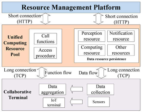
Figure 2.
Optimize resource pool models.
- (1)
- Data flow: The computing resource pool performs persistent processing of various sensor fusion data uploaded by collaborative terminals, completes data storage, and the stored data can be viewed through the resource management platform for status and parameters. Resource pool data persistence collects terminal device data into the resource pool and realizes data management and control through the resource management platform. This method can realize centralized storage, facilitate data management and sharing, and realize the expansion of storage space at the same time. It can effectively access massive data from multiple terminals and ensure high operation efficiency. Resource pool data persistence also makes the data more secure and reliable, reducing the pressure on the platform.
- (2)
- Function flow: Through the transmission of terminal information through the data flow, the platform side can confirm the offline and online status of the terminal. However, the operation and control of the terminal cannot be completed through the data flow. The control of the terminal needs to call the controllable terminal access function and simultaneously confirm that the terminal status is online and realize the parameter configuration and device management of the access terminal through the interface program docking with the platform.
In order to complete multi-terminal data fusion, we must first enable the application platforms of different terminals to access the resource pool. This process requires the development of a middleware toolset to connect the application platform, the unified computing resource pool, and the resource management platform. The overall processing flow is shown in Figure 3.

Figure 3.
Resource Device Flow.
Through the optimized design of the unified computing resource pool model, the complexity of the terminal access platform can be significantly reduced, the amount and efficiency of terminal access can be greatly improved, and it can effectively solve the problems of the number of terminals and daily surge, information data resources causing information congestion, low resource management efficiency, and other issues. However, this model has higher requirements on the terminal, and the terminal needs to perform information localization processing and complete specific data collection.
3. PSO—BP Neural Network Algorithm
3.1. Principle of Particle Swarm Optimization Algorithm
Particle swarm optimization [17] regards individuals in a flock as particles in a local space, and food can be regarded as the optimal solution for the space. The basis of particle velocity and position adjustment is that two extreme values update each particle during each iteration. By judging the solution under these two extreme values, the particle’s speed and position are updated and adjusted until the position of the optimal solution is reached. The velocity and position update formulas are shown in (1) and (2), respectively:
In the above formula: is the particle velocity; is the optimal position of the particle; is the optimal particle swarm search position; and are called learning factors, which are used to represent the moving step size of particles to the optimal global value; and are arbitrary numbers between sets [0, 1]; k represents the number of iterations; and represent the optimal value of the extreme individual value and the optimal global value respectively. The first term in Formula (1) is the particle velocity of the k-th iteration, and the second term indicates that the particle is affected by itself and adjusts the speed, and the third term indicates that the particle is affected by the group to adjust the speed. The position of the particle is updated as shown in Figure 4:
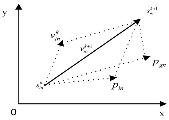
Figure 4.
Particle position iterative update process.
3.2. Principle of BP Neural Network Algorithm
BP neural network [18,19,20], the most widely used model in neural network algorithms, is developed based on the idea of simulating the composition of the human brain. The BP neural network continuously learns from many samples, adopts the backpropagation method to optimize the weights of the BP neural network and update the threshold value, and uses the steepest descent method to make the predicted output continuously approach the actual output. The BP neural network can be divided into three layers: the input layer, the output layer, and the hidden layer. Weights can connect each layer, but the layers do not correlate. The simplest network structure is shown in Figure 5:

Figure 5.
Topology of BP neural network.
The input and output layers of the BP neural network belong to a single-layer structure, and the hidden layer is generally a multi-layer structure. Generally speaking, the higher the number of hidden layers, the higher the accuracy of the operation, but it will also affect the training time. There is no unified specification for the selection of hidden layer nodes, and the number of hidden nodes is usually determined according to the following formula:
The above formula: is the number of input nodes; is the number of output nodes; and is any number, usually with the value [0, 10]; is the number of hidden layer nodes.
The advantage of the BP neural network algorithm is that it has a strong non-fault mapping ability; it can perform autonomous training and has relatively strong learning ability, and it also has certain fault tolerance, but the biggest defect of the BP neural network is that the adjustment of weights and thresholds is easy to fall into local optimal, resulting in unsatisfactory system training results. In order to avoid the above defects, optimizing the weights and thresholds of the BP neural network is necessary.
3.3. PSO–BP Neural Network Optimization Algorithm
The BP neural network has the defect that it is easy to fall into the local optimum when the weights and thresholds are adjusted. In the particle swarm algorithm, the particles are optimized globally, and the optimal value of the particle itself is compared with the optimal global value, which has the advantage of real-time updates. Suppose the PSO algorithm and the BP neural network algorithm were combined. In that case, the weights and thresholds of the BP neural network are regarded as the position information of the particles, and the particles find the optimal solution globally, update the position information, and achieve the adjustment of the threshold and weight. To a certain extent, the defects of the BP neural network are avoided. The flow chart of the BP neural network optimized by PSO is shown in Figure 6.
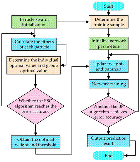
Figure 6.
Flow chart of BP neural network optimized by PSO.
The steps of the PSO–BP algorithm are shown in Algorithm 1 [21].
| Algorithm 1. The steps of the PSO–BP algorithm. | |
| 1: | Initialize the BP neural network structure: determine the network structure, the number of hidden layer nodes, the number of iterations and accuracy, and the learning rate; |
| 2: | Initialize the particle swarm algorithm: determine the size of the particle swarm (affected by the BP network input, output, and the number of hidden layer nodes), the maximum number of iterations, accuracy, particle velocity range, position range, and other parameters; |
| 3: | Calculate the fitness of the particle swarm to find the optimal value of the particle itself and the optimal global value; |
| 4: | If the accuracy of the PSO algorithm meets the requirements or reaches the maximum number of iterations, end the PSO algorithm and obtain the optimal parameter values. If it does not meet the requirements, update the particle velocity and position information, and recalculate particle fitness; |
| 5: | Update the weight and threshold information of the BP network through the optimal parameter values obtained by PSO and determine whether the error accuracy or the maximum number of iterations of the BP–PSO network meets the requirements. If satisfied, end the training; |
| 6: | Output the prediction result. |
4. Fault Analysis of Distribution Network Equipment
4.1. Fault Diagnosis of Transformer Based on PSO–BP
4.1.1. Analysis of the Generation Mechanism of Dissolved Gas in Transformer Oil
Through chemical bonds, transformer insulating oil is a multi-molecular mixture composed of carbon and hydrogen atoms. When the transformer operates under normal conditions, the heat generated is low, and it will not cause many hydrocarbons and carbon–carbon chemical bonds to break. The insulating oil can be stable in operation. When a fault occurs inside the transformer, the transformer oil is heated, or there is a discharge phenomenon inside, which will easily split the C–H chemical bond and the C–C chemical bond in the molecule, resulting in carbon atoms and hydrogen atoms, unstable free radicals, etc. These unstable carbon, hydrogen atoms, and free radicals combine to form various gases, called characteristic gases, usually including hydrogen, carbon oxides, and various hydrocarbon gases, and with the further development of internal failures, the resulting gas content will gradually increase. Therefore, the composition, relative content, and gas production rate of characteristic gases can be used as the basis for judging transformers’ internal faults.
According to the nature of faults, transformer faults can be divided into overheating faults and discharge faults. Generally, thermal faults are divided into three types according to the temperature of the fault point: low-temperature overheating (T < 300 °C), medium-temperature overheating (300 °C < T < 700 °C) and high-temperature overheating (T > 700 °C) faults. Both experimental research and practice have shown that when the temperature of the fault point is low, the oil’s dissolved gas composition is mainly CH4. As the temperature increases, the gases with the highest gas production rate are CH4, C2H6, C2H4 and C2H2 in sequence. Because C2H6 is unstable, it easily decomposes into C2H4 and H2 at a specific temperature. Therefore, the content of C2H6 in oil is usually less than CH4, and C2H4 and H2 are always accompanied. When the transformer is overheated at a low temperature, the ratio of H2 in the transformer oil to the total amount of hydrogen hydrocarbons is higher than 27%. In the case of medium and high-temperature overheating faults, H2 accounts for less than 27% of the total hydrogen hydrocarbons. When the high temperature is superheated, the characteristic gas is mainly C2H4, followed by CH4, and the sum of the two generally accounts for more than 80% of the total hydrocarbons. In addition, there are C2H6 and H2. When overheating is severe, a small amount of C2H2 will also be produced, and its entire content is at most 6% of the total hydrocarbons. Discharge faults can be divided into low-energy discharge and high-energy discharge. Low-energy discharge includes partial discharge and sparks discharge. When low-energy discharge occurs, the leading characteristic gases are H2 and CH4, and C2H4 gas is rarely produced. Arc discharge is high-energy discharge. When high-energy discharge occurs, a large amount of H2, CH4 and C2H4 will be produced. When the transformer is overheated and discharged, the characteristics of the dissolved gas components in the oil are shown in Table 1.

Table 1.
Corresponding gas relationship of different fault types.
The gas content of the transformer changes under different faults, mainly H2, C2H4, CH4, C2H6, C2H2, CO, CO2, O2, N2. O2 and N2 exist in large quantities in the normal state of the transformer. Under different fault types, the two gases do not change significantly, so this paper does not consider these two gases. CO2 and O2 also only change significantly for the overheating and high-energy discharge of solid insulating materials, so these two gases do not need to be considered. In summary, only the contents of H2, C2H4, CH4, C2H6 and C2H2 were considered, and the concentrations of these five gases were selected as their characteristic vectors. That is, the number X of network input nodes is five.
We divide the transformer diagnosis result output into one normal and five fault states, so there are six output states. The PSO–BP algorithm needs to output the result in binary form, and the transformer output fault codes are shown in Table 2.
Table 2.
Coding value of transformer fault output.
When the transformer is in different faults, the gas content in the oil varies greatly, showing a highly skewed distribution. We need to normalize the data to consider the difference in gas content. The most commonly used methods for processing highly skewed data are arctangent transformation (AT), logarithmic transformation (LT), and linear normalization. For the AT transformation method, such as Formula (5):
the sample data can be limited to [−/2,/2] by taking the arctangent transformation.
For the LT transformation method, such as Formula (6):
For the linear normalization method, such as Formula (7):
the data is limited to [−1, 1] by linear normalization.
Considering the characteristics of the BP algorithm, the linear normalization algorithm was chosen in this paper.
From the 169 groups of data collected, 131 groups were selected for network training, and the remaining 38 groups were used for testing. The number of each failure sample in the test set and training set is shown in Table 3.
Table 3.
Test set and training set sample allocation.
The parameters in the PSO–BP algorithm will affect the accuracy and diagnosis time of the system, so it is essential to select the system parameters. In this paper, aiming at transformer fault diagnosis, the best diagnostic performance was obtained by continuously modifying the parameters. We set the arithmetic as follows: the learning factors c1 and c2 were set to 2; the maximum number of iterations was 100; the number of particles was 20; and the number of hidden layer nodes was determined according to Formulas (3) and (4). According to the established transformer diagnostic model, it can be known that x = 5 and y = 5 are in Formulas (3) and (4). The value range of m was a constant between [0, 10], and the number of hidden layer nodes was between [3, 13]. Through continuous testing of the model, when the number of nodes in the hidden layer was four, the convergence degree of the diagnostic system was the highest, and the error was the smallest.
4.1.2. Analysis of Transformer Fault Diagnosis Results
- (1)
- Analysis of the Diagnostic Results of PSO–BP
In the constructed transformer fault diagnosis model, using the PSO–BP algorithm, the diagnostic results of the test set and a training set of the transformer are shown in Figure 7.
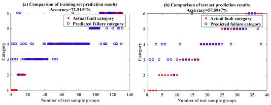
Figure 7.
PSO–BP transformer diagnostic results.
As seen from the Figure 7, with the gas concentration in the oil as the characteristic quantity, the diagnostic accuracy rates of the training and diagnostic samples were 72.52% and 57.89%, respectively. The diagnosis accuracy rate was not high, and the diagnosis effect was not ideal.
The change rule of the mean square error curve of the PSO–BP algorithm is shown in Figure 8.
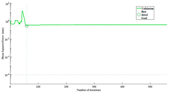
Figure 8.
Variation of mean square deviation curve.
It can be seen from Figure 8 that when the number of iterations of the system was 59, convergence was achieved at this time, and the mean square error was only 0.28046.
The fault diagnosis of the transformer was carried out with the gas concentration as the characteristic quantity, and the result was very unsatisfactory. The diagnosis accuracy rate of the training set and the test set was relatively low, and the convergence accuracy of the mean square error curve was poor.
- (2)
- Analysis of diagnosis results of BP algorithm
Because the weights and thresholds in the BP algorithm often fall into local optimum, the output of each diagnosis result was not completely consistent. Therefore, we take the average value of the correct rate of 10 simulations, and the simulation results of the 10 simulations are shown in Figure 9.

Figure 9.
BP algorithm diagnosis results.
Using the BP neural algorithm for fault diagnosis, the correct average training and test sample rates were 55.50% and 37.89%, respectively. Compared with the PSO–BP algorithm, the diagnostic accuracy rate decreased by 17.02% and 20.00%. Therefore, the PSO algorithm can improve the accuracy of the diagnosis results compared with the BP algorithm.
4.1.3. Optimization of Fault Feature Quantity Based on PSO
After selecting and preprocessing the transformer data feature quantity, we optimized the transformer fault feature quantity. In this paper, the continuous PSO algorithm was selected, which can realize the simultaneous adjustment of particle velocity and position. Compared with the discrete PSO algorithm, the algorithm has the characteristics of simple parameter adjustment and easy implementation.
The essence of feature quantity optimization is to calculate the influence factor of each feature quantity on the target result through the optimization algorithm. The influence factor sorts the feature quantities, the feature quantity with a relatively high influence factor is retained, and the feature quantity with a relatively low influence factor is removed. The limit set in this article was 0.5; elements larger than 0.5 were kept, and elements smaller than 0.5 were eliminated. The parameters of the PSO algorithm were set as follows: learning factors , ; the total number of particles was 30; the initial value of particle inertia was 1; the inertia decay rate was 0.9; and the maximum number of iterations in a PSO optimization was 50 times.
We used the PSO algorithm to find the best subset of input features. The initial particles of the PSO algorithm were randomly generated. In order to improve the optimization effect, the PSO optimization algorithm was run independently 15 times, and the optimal subset corresponding to the maximum value of the objective function was taken as the optimal feature vector group. The preferred vectors corresponding to the first four bits of the objective function value are shown in Table 4.
Table 4.
Results of feature optimization.
- (1)
- Comparative analysis of results of different preferred subsets
We used the PSO algorithm to select four sets of feature subsets. According to the distribution of various fault data in Table 4, the training set and test set of four sets of feature subset samples were determined (the selection was consistent with the selection of the training set and test set with the characteristics of gas concentration). Moreover, we used the sample output accuracy of the PSO–BP algorithm to determine the best-preferred subset. The results of each subset of diagnostic test samples and diagnostic samples are shown in Figure 10.
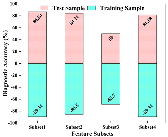
Figure 10.
Sample accuracy comparison analysis of different feature subsets [1].
It can be seen from Figure 10 that the correct rate of training samples and test samples for each preferred subset except feature subset 3 was above 80.00%. The diagnostic and test samples of the preferred feature subset 1 had the highest correct rates, 89.31%, and 86.84%, respectively. Therefore, feature vector 1 was selected as the optimal feature subset.
- (2)
- Comparative analysis of optimal feature subset and gas concentration feature diagnosis results
This paper selected feature subset 1 as the best subset, and the training samples and test accuracy of the best feature subset are shown in Figure 11.
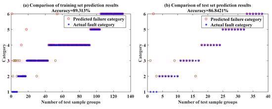
Figure 11.
Transformer optimal feature subset fault diagnosis results.
The correct rates of test and diagnostic samples of the preferred vector were 89.31% and 86.84%, respectively. The correct rates of test and diagnostic samples characterized by gas concentration were 72.52% and 57.89%, respectively. Compared with the diagnosis accuracy rate characterized by gas concentration, the diagnostic accuracy rate of the optimal vector increased by nearly 16.79% and 49.97%. It was proved that the optimal Eigenvector group using PSO can improve the diagnostic accuracy compared with the input quantity characterized by concentration.
4.2. Fault Diagnosis of Circuit Breaker Based on PSO–BP
4.2.1. Circuit Breaker Diagnosis Model Based on PSO–BP
According to statistics [22], the faults of vacuum circuit breakers are mainly related to the operating mechanism and its auxiliary circuits. Nearly 45% are mechanical faults, and 23% are faults caused by auxiliary circuits. Abnormal operating mechanisms cause most mechanical failures of vacuum circuit breakers. During the closing and opening operation of the circuit breaker, current will flow through the opening and closing coil, and a magnetic flux will be generated in the iron core, which will change the action of the iron core and the spring device. Therefore, the opening and closing coil currents change to a certain extent. The operating state of the magnet iron core and the opening and closing spring of the operating structure can be reflected in the upper part. Therefore, the current characteristics of the closing and opening coils can be selected as the characteristic quantities of the fault diagnosis of the vacuum circuit breaker. The change curve of the coil current is shown in Figure 12.
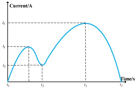
Figure 12.
Coil current curve.
In the vacuum circuit breaker, the current variation characteristics of the opening and closing coils corresponding to each fault type are as follows:
- (1)
- The supply voltage of the operating mechanism is too low. The working conditions of the circuit breaker are poor, the independent power supply applied by the opening and closing coil is easily affected by the environment, and the applied voltage source is lower than the specified value. If the voltage of the opening and closing coil is too low, the time difference in Figure 12 will increase, the coil current will be lower than the standard value, the energization time of the iron core and the operation time of the circuit breaker will increase, and the circuit breaker cannot operate within the specified time.
- (2)
- The operating mechanism is jammed. The jamming of the operating structure will not change the coil current curve, and the size of the coil current will not change, but it will increase the total travel time.
- (3)
- Coil failure. When there is a fault in the coil, the equivalent resistance of the coil increases, resulting in a decrease in the coil current and an increase in the opening and closing time.
- (4)
- The auxiliary switch is in poor contact. Suppose the auxiliary switch is in poor contact. In that case, the coil power supply cannot be cut off, the circuit breaker cannot perform the closing operation, and the section of the current characteristic curve is elongated. If the situation is more serious, it will eventually cause the circuit breaker to burn out.
Among the above faults, the coil current change curves corresponding to the too-low supply voltage of the operating mechanism and the jamming fault of the operating mechanism are shown in Figure 13. Figure 14 shows the change curves of the coil current corresponding to the fault of the coil and the fault of poor contact of the auxiliary switch.
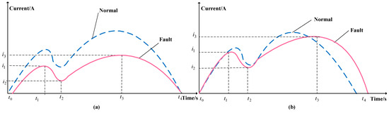
Figure 13.
Comparison of fault opening and closing coil current and normal waveform: (a) Comparison of low supply voltage of operating mechanism and normal waveform; (b) Comparison of operating mechanism jam and normal waveform.
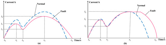
Figure 14.
Comparison of current waveform of closing coil under various faults: (a) Comparison of closing coil fault and normal waveform; (b) Comparison of poor contact of auxiliary switch and normal waveform.
4.2.2. Circuit Breaker Diagnosis Model Based on PSO–BP
The circuit breaker’s opening and closing coil current contains rich fault information. By analyzing the waveform of the opening and closing coil current, the diagnosis of some mechanical faults of the circuit breaker can be realized. In this paper, the critical inflection point information of the opening and closing coil current was selected as the input quantity of the fault diagnosis model: current quantity information (i1, i2, i3) and important time nodes (t1, t2, t3, t4). Since the final output of the PSO–BP algorithm is in binary form, the encoding form is shown in Table 5.
Table 5.
Fault code of circuit breaker.
The research on the fault diagnosis of circuit breakers is relatively late, and less sample data exists of mechanical fault diagnosis of the opening and closing of coils. We obtained 30 sets of data from the literature [23] as the total sample data. In the PSO–BP algorithm, the parameters will affect the accuracy and diagnosis time of the system, so it is essential to select the system parameters. According to the characteristics of the mechanical fault diagnosis of the circuit breaker, we set the parameters as shown in Table 6.
Table 6.
PSO–BP parameter settings.
4.2.3. Analysis of Circuit Breaker Diagnosis Results
In this paper, 30 groups of data were collected as sample data; the first 20 groups of data were training samples, and the last 10 groups were test samples. The distribution of the number of each fault type for training samples and test samples is shown in Table 7.
Table 7.
Sample allocation of test set and training set [1].
The systematic error curve of the diagnostic analysis of the PSO–BP algorithm is shown in Figure 15.

Figure 15.
Variation of mean square deviation curve.
It can be seen from Figure 15 that when the number of iterations was the 7th, the system reaches convergence, and the corresponding mean square error at this time was 0.038. The diagnostic results of test samples and training samples are shown in Figure 16.
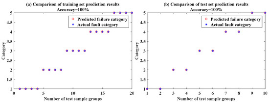
Figure 16.
Diagnosis result analysis of training set and test set.
Among the 10 groups of data in Figure 16, there were two groups of TD, GD, CF, CKS, and FK, and the diagnosis results were entirely consistent with the actual fault.
The first 20 groups of data were selected as training samples, and the last 10 groups were selected as test samples, and the diagnosis results were entirely consistent with the actual faults. On this basis, this paper analyzed the influence of different training sample numbers on the diagnosis results. The samples with serial numbers 4, 8, 12, 16, and 20 were merged into the test samples, and the test samples and training samples were both 15 sets of data. The diagnostic results of the test set and sample set are shown in Figure 17.
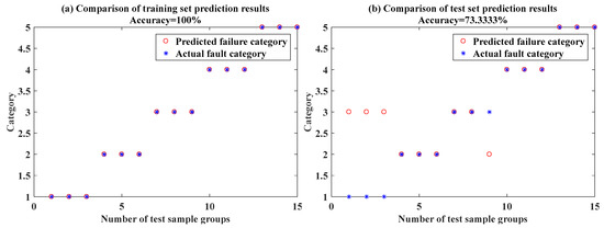
Figure 17.
Analysis of diagnosis results with different number of samples.
It can be seen from Figure 17 that when there were 15 training samples and 15 testing samples, there were four diagnostic errors in the test set samples, and the diagnostic accuracy rate was only 73.33%. Therefore, the number of test samples and diagnostic samples will have an impact on the diagnostic sample accuracy rate.
5. Conclusions
Based on the IoT and multi-data fusion technology, this paper establishes a fault diagnosis model for transformers and circuit breakers for two critical pieces of equipment in the traction power supply system: transformers and circuit breakers. The conclusions are as follows:
- This paper studies the unified computing resource pool technology and multi-data fusion technology, and proposes a fault diagnosis framework for power equipment based on the IoT.
- Using a PSO–BP algorithm to realize transformer fault diagnosis. Taking the gas concentration as the characters as the input, the diagnostic accuracy rates of the test set and the sample set were 72.52% and 57.89%, respectively. Therefore, compared with the PSO–BP algorithm, the diagnostic accuracy rate was 17.02% and 20.00% higher than that of the BP algorithm. It has been proved that the PSO algorithm can optimize the BP algorithm and improve the diagnosis results’ accuracy.
- Transformer feature optimization is realized by PSO. For 26 kinds of transformer concentration feature quantities, the optimal feature subset was determined by PSO, and the diagnostic accuracy rates of the training set and test set of the optimal feature subset were 89.31% and 86.84%, respectively, improving the accuracy of transformer fault diagnosis.
- The fault diagnosis model of the circuit breaker was established using the PSO–BP algorithm. The number of training sets and test sets was 20 groups, respectively, and the diagnostic accuracy rates were 100%, and 100% when the number of training sets and test sets was 10 groups, respective. When the number of training sets and test sets was 15 groups, respectively, the correct diagnostic rates were 100% and 73.33%. It has been proved that different sample sizes impact the diagnostic results.
The abnormal operation of electrical equipment will affect the power quality and even endanger personal safety, so the research on the diagnosis of abnormal equipment is of great significance.
Author Contributions
Conceptualization, Z.X. and Z.Z.; methodology, Z.Z., Z.X. and W.W.; software, Z.Z. and Z.X.; validation, Z.Z. and Z.X.; formal analysis, Z.W. and W.W.; investigation, T.X.; resources, Z.W.; data curation, Z.Z. and T.X.; writing—original draft preparation, Z.Z.; writing—review and editing, Z.Z., W.W. and Z.X.; visualization, Z.Z.; supervision, Z.W.; project administration, Z.W.; funding acquisition, Z.W. All authors have read and agreed to the published version of the manuscript.
Funding
This research was supported by National Key Research and Development Program 2018YFB2100100.
Data Availability Statement
Not applicable.
Conflicts of Interest
The authors declare no conflict of interest.
References
- Wu, Z.; Zhang, Z.; He, J.; Yue, B. Transformer Fault Diagnosis Algorithm for Traction Power Supply System Based on IoT. In Proceedings of the 5th International Conference on Electrical Engineering and Information Technologies for Rail Transportation (EITRT), Qingdao, China, 22–24 October 2021; Lecture Notes in Electrical Engineering. Volume 864, pp. 637–644. [Google Scholar]
- Ashkezari, A.D.; Ma, H.; Saha, T.K. Investigation of feature selection techniques for improving efficiency of power transformer condition assessment. IEEE Trans. Dielectr. Electr. Insul. 2014, 21, 836–844. [Google Scholar] [CrossRef]
- Cheng, S.; Cheng, X.; Yang, L. Application of wavelet neural network based on improved particle swarm algorithm in transformer fault diagnosis. Power Syst. Prot. Control. 2014, 42, 37–42. [Google Scholar]
- Liu, K.; Peng, W.; Yang, X. Application of Feature Optimization and Fuzzy Theory in Transformer Fault Diagnosis. Power Syst. Prot. Control. 2016, 44, 54–60. [Google Scholar]
- Gu, K.; Guo, J. Transformer Fault Diagnosis Based on Compact Fusion Fuzzy Set and Fault Tree. High Volt. Technol. 2014, 40, 1507–1513. [Google Scholar]
- Zhao, W. Transformer Fault Diagnosis Based on Selective Bayesian Classifier. Electr. Dig. 2011, 5, 34–37. [Google Scholar]
- Huang, N.; Chen, H.; Cai, G. Mechanical Fault Diagnosis of High Voltage Circuit Breakers Based on Variational Mode Decomposition and Multi-Layer Classifier. Sensors 2016, 16, 1887. [Google Scholar] [CrossRef]
- Kim, S.; Seo, H.; Jung, J.; Yang, H. New methods of DGA diagnosis using IEC TC 10 andrelated databases Part1: Application of gas-ratio combinations. IEEE Trans. Dielectr. Electr. Insul. 2013, 20, 685–690. [Google Scholar]
- Lee, S.; Seo, H.; Jung, J.; Yang, H. New methods of DGA diagnosis using IEC TC 10 andrelated databases Part2: Application of gas-ratio combinations. IEEE Trans. Dielectr. Electr. Insul. 2013, 20, 691–696. [Google Scholar]
- Sifat, I.M.; Mohamad, M.A. Circuit breakers as market stability levers: A survey of research, praxis, and challenges. Int. J. Financ. Econ. 2019, 24, 1130–1169. [Google Scholar] [CrossRef]
- Sun, L.; Hu, X.; Ji, Y. Application of improved wavelet packet-characteristic entropy in fault diagnosis of high-voltage circuit breakers. Chin. J. Electr. Eng. 2007, 12, 103–108. [Google Scholar]
- Liu, Q.; Peng, Z.; Wang, S. Identification of fault current curve of circuit breaker opening and closing coil based on random forest algorithm. High Volt. Electr. Appl. 2019, 55, 93–100. [Google Scholar]
- Xu, K. Research on High-Voltage Circuit Breaker Remote Condition Monitoring System and Fault Diagnosis Technology; Nanjing University of Science and Technology: Nanjing, China, 2019. [Google Scholar]
- Dong-Hyuk, I.M.; Lee, S.W.; Kim, H.J. A version management framework for RDF triple stores. Int. J. Softw. Eng. Knowl. Eng. 2012, 22, 85–106. [Google Scholar]
- Liu, F. Research and Prospect of Multi-sensor Information Fusion Technology. Ind. Technol. Forum 2014, 13, 69–70. [Google Scholar]
- Wu, H.; Zhang, S. Design of smart city management system based on cloud computing platform. Inf. Technol. 2021, 10, 95–99. [Google Scholar]
- Sun, Y.; Chen, X.; Yang, S. Micro PMU based monitoring system for active distribution networks. In Proceedings of the IEEE 12th International Conference on Power Electronics and Drive Systems (PEDS), Honolulu, HI, USA, 12–15 December 2017. [Google Scholar]
- Yang, C.; Li, Y.; Yang, B. Dynamic variable-weight least squares for state estimation of distribution network based on data fusion. In Proceedings of the IEEE Conference on Energy Internet and Energy System Integration (EI2), Beijing, China, 26–28 November 2017. [Google Scholar]
- Wang, Y. Research on Distribution Network State Estimation Method Based on PMU/SCADA Measurement Data; Beijing Jiaotong University: Beijing, China, 2019. [Google Scholar]
- Yang, Y.; Lei, X.; Xu, G. Multi-objective power optimization scheduling of microgrid using PSO-BF algorithm. Power Syst. Prot. Control. 2014, 42, 13–20. [Google Scholar]
- Yang, Q. Research and Application of Improved PSO-BP Neural Network in Transformer Fault Detection; Chongqing University: Chongqing, China, 2010. [Google Scholar]
- Zeng, Q.; Lin, Y.; Zhao, Y. On-line monitoring of mechanical characteristics of circuit breakers and feature extraction of vibration signals. J. Huazhong Univ. Sci. Technol. 2009, 37, 118–121. [Google Scholar]
- Jiang, H.; Li, T.; Cheng, H. Mechanical fault diagnosis of spring mechanism of high voltage vacuum circuit breaker based on PSO-LSSVM. High Volt. Electr. Appl. 2019, 55, 248–255. [Google Scholar]
Publisher’s Note: MDPI stays neutral with regard to jurisdictional claims in published maps and institutional affiliations. |
© 2022 by the authors. Licensee MDPI, Basel, Switzerland. This article is an open access article distributed under the terms and conditions of the Creative Commons Attribution (CC BY) license (https://creativecommons.org/licenses/by/4.0/).