Abstract
Projects that feature unconventional geothermal systems are complex and come at great investment risk and high project cost. The purpose of this work is to present a method for modelling an enhanced geothermal system (EGS) that utilizes a horizontal well-doublet setup. The proposed wells’ positioning was to minimize one of the biggest cost factors: the flow rate. As a part of the research, a case study was conducted and a fully coupled EGS model prepared, based on the data from the Utah FORGE site. The model includes a discrete fracture network (DFN) that represents hydraulic fractures and a stimulated reservoir volume (SRV) for controlling the fractures’ properties. The model’s viability was checked by a series of reservoir simulations, which provided the results for sensitivity analysis of the production parameters. Analysis of the results was conducted based on the temperature decline over an EGS system lifetime, which is one of the primary indicators for EGS. The proposed solution allowed for effectively minimising the injection and production flow rate while maintaining reasonable temperature drawdown levels. It was proven that reservoir modelling and simulation tools, used in the oil and gas industry, can be successfully applied for modelling geothermal systems.
1. Introduction
Geothermal energy, compared to other renewable energy sources, has a great potential to dominate the global energy supply in the future. It can provide a safe and sustainable way for long-term energy utilization, is not as location-dependent as wind or solar energy, and can be more accessible than many hydrocarbon reservoirs [1]. Conventional geothermal systems have been exploited commercially for many years, so their behaviour is well understood by now. The unconventional resources usually feature much higher temperatures, indicating a higher energy recovery rate, which, on the other hand, involves more technological and economic challenges. Enhanced Geothermal System (EGS) is an example of an unconventional geothermal resource and refer to conduction dominated, low permeability basement formations (petrothermal) but also include geopressured systems and a low grade, unproductive hydrothermal formation [2,3].
1.1. Petrothermal EGS Characteristics
The usual way in which Enhanced Geothermal System operates requires a set of two wells (injection and production well) positioned a few meters apart. The wells have to be connected through a network of hydraulic fractures that assures the hydrodynamic communication between them. The last essential element is the working fluid, which is usually water or CO2. The fluid functions as an energy carrier and transports heat absorbed from the rock matrix up to the surface equipment [4]. A typical development setup of an EGS reservoir is presented in Figure 1.
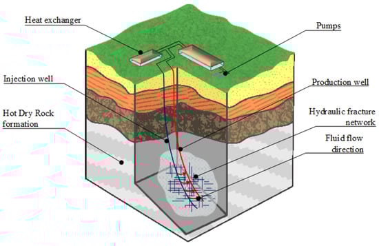
Figure 1.
A typical enhanced geothermal system setup with a doublet of deviated wells [2].
Usually, the first step in an EGS project development is the investigation of geological and geomechanical properties of the selected location and specifying if a relevant bedrock formation is present. After the preliminary research is completed, the exploration phase is being conducted to identify the best possible sites for production. To achieve this, a test well is drilled to the depth of 3–10 km where adequate temperatures and bedrock formation are typically found [3]. Thermal energy at these depths is most often stored in granitic or tight sandstone formations that have low or very low permeability and require enhancement to assure flow in the formation. Depending on whether original fluids in place are present or not, the encountered geothermal system may be defined either as hydrothermal or petrothermal [5]. If the testing phase confirms that HDR structure is in place, the prediction models forecast that thermal energy is accessible and extractable with profit, then the Enhanced Geothermal System is developed. To achieve this drilling of the second well, fracturing operation is required. Hydraulic fracturing improves the formation’s natural permeability by creating an artificial network of fractures or shearing the natural fractures, present in the formation. Understanding of the EGS technology is improving, and numerous approaches to this method are currently under research. Many of them originate from the Oil and Gas industry since the technology features solutions already investigated during petroleum operations [3]. The research presented in this article is an attempt to introduce a novel way of EGS development utilizing a horizontal well-doublet and demonstration of a method to model such system, using the standard modelling and simulation tools used in petroleum engineering [2].
1.2. EGS Modelling Methods
Over time, numerical simulation tools used in EGS modeling became more advanced and can provide more accurate and rational EOS for the fluid flow and heat transfer. For hydrothermal cases, the TOUGH2 code, TETRAD, STAR, and FEHM are the commonly used simulators, out of which, the most popular is TOUGH2 [6]. The TOUGH2 simulator was developed by the US Department of Energy and applies to geothermal reservoir simulation cases, but also groundwater and nuclear waste pits modelling. It allows fully coupled modeling of the multi-component and multi-phase fluid and heat flow in one, two or three-dimensional geometry of porous or fractured reservoirs [2,7].
The major challenge in the EGS reservoirs simulation was to reflect the permeability improvement achieved by the creation of artificial fractures which disallowed modelling the fracture network as an effective continuum and forced the explicit approach to be introduced. Explicit approaches usually involve the application of discrete fracture models and fracture grid refinement [8]. One of the standard methods for fracture network modeling is the application of the MINC (Multiple Interactive Continua) approach, featured in TOUGH2 code. It allows a modeling temperature transition between the hot rock matrix and cold injected fluid by matrix sequential partitioning [2,8]. The MINC method is an extension of the original double-porosity concept [9] which overcomes the quasi-steady limitation for multiphase, non-isothermal flow by computing the fluid flow in the porous structure in a fully transient way, by using the numerical approximation of the principal flow properties such as pressure and temperature gradients [10]. Currently, the most popular method for modelling hydraulic fractures in geothermal, especially HDR/EGS reservoirs is the Discrete Fracture Network (DFN) method. DFN refers to a numerical model that computes the individual fracture properties such as size, width, and orientation explicitly and represents the geometrical relationships between the fracture planes [11]. The DFN approach has proven to be applicable for modelling the heat extraction from the EGS reservoirs through hydraulic fractures and recent studies of Gong et al. [12] and Yao et al. [13] are excellent evidence for that. Yao et al. [13] had used discrete fracture modelling for creating a 2D fracture surface that would reflect the heat transfer through fluid circulation only in the dominant flow channel. In the work of Gong et al. [12], a Discrete Fracture Model was used to imitate the fractured geothermal reservoir, with isotropic fractures in a homogeneous rock matrix, while the reservoir was represented by a set of nodal points (finite element mesh) with the discrete fractures incorporated as two-dimensional boundary faces [12,13]. In addition, the model used by Gong et al. [12] consisted of a stimulated reservoir volume (SRV), which is an empirical replacement that allows good accuracy in modelling of the complex fracture networks [2,12]. One of the most recent works focusing on the horizontal wells fracturing optimization including the use of the SRV was published by Zhang and Sheng [14]. In their paper, a comprehensive analysis of the SRV effect on horizontal well optimization was suggested, and a mathematical model for estimating the Stimulated Reservoir Volume was proposed. They have established that SRV can be evaluated by combining the induced stress model, natural fracture durability, and hydraulic pressure model [2,14].
1.3. Horizontal Well-Doublet EGS
This article proposes a novel setup for an EGS reservoir development that includes a distinctive way of wells positioning and presents a sensitivity analysis of the primary production parameters. The main idea behind this research is to use the horizontal wells technology in the EGS reservoir, which was already considered in several articles on EGS modelling approaches [12,15,16,17,18]. However, this setup has been examined only for wells located parallel in the vertical plane or in the horizontal plane but with the injection well located below the production well. The proposed setup assumes using two horizontal wells located one above the other with the injection well located above the production well so that the working fluid streams down through the fracture network not only with the help of injection rate and pressure but also as an effect of the gravitational force presence and have an impact of injected fluid properties, where increasing temperature leads to change in fluid phase properties and generally creates more favorable flow conditions. Visualization of the proposed solution is presented in Figure 2.
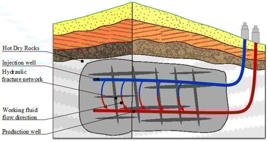
Figure 2.
Proposed well setup for EGS system development with a horizontal well-doublet [2].
Since the article proposes a novel way of EGS development that would require different operating parameters, from the standard approach, the sensitivity analysis of these parameters is included, in order to investigate their impact on the system’s performance [2].
2. Methodology
2.1. Utah FORGE Project
The Utah FORGE site was chosen as a source of the data for this work because the main focus of the FORGE project is to deliver an effective way of EGS utilization and finding the applicable solutions for the commercialization of this technology. Along with the fact that the Utah FORGE site features ideal conditions for an EGS reservoir development and meets all the requirements specified by the United States DOE, FORGE data sets provide great conditions for conducting research on EGS [2,19]. The data sets are available to use for research purposes under open license and are accessible at Geothermal Data Repository (GDR) [20].
The site of the project lays on sloping alluvial sediments and is located in between the Milford valley and crest of the Mineral Mountains. Local lithology consists of two major geological formations, the overlying alluvial sedimentary deposits, and basement granitic rock formation, broadly referred to as granitoid. The crystalline basement formation is dominated by the granitic rocks, mainly from the Miocene age, which are also the core of the Mineral Mountains. Two faults have been identified in the area of the project’s site: the Opal Mound fault and Negro Mag fault. These relatively short structures form natural boundaries between the Roosevelt Hot Springs hydrothermal system and the approximate location of the petrothermal EGS reservoir. Figure 3 presents a cross-section of the site location alongside with the location of the reference well for this work—58-32, as well as the approximate location of planned EGS reservoir [2,19]. All of the Utah FORGE data used in this research is open-sourced and available at Geothermal Data Repository [20].
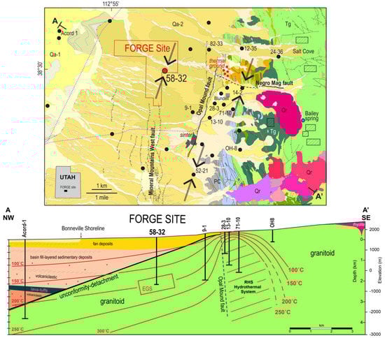
Figure 3.
Upper: Geological map of the Utah FORGE site area; Lower: Cross section of the Utah FORGE site area. Maximum horizontal stress is highlighted with the black arrows. Beige (Qa-1): silts and sands of Lake Bonneville; Yellow (Qa-2) fan deposits; Purple (Qr): Quaternary rhyolite lava; Dark teal and spring green (Tg): Tertiary granitoid; Grey (PC): Precambrian gneiss; wells are highlighted as black circles; only the reference 58-32 well is a red circle. Red rectangle in the cross section represents an approximate location of the planned enhanced geothermal system and the thermal profiles are represented by red lines [19].
2.2. Structure of the Model
2.2.1. Conceptual Model
The target simulation model is an excerpt of the FORGE project’s granitoid formation, limited by two temperature profiles (isotherms) between which the planned EGS reservoir is about to be located. The model utilizes the SRV concept which is achieved by introduction of the local grid refinement in the separated region, outside of which no-flow conditions are applied. The modelled setup is presented in Figure 4, along with the unique positioning of the horizontal wells. A discrete hydraulic fracture network is included in the SRV and intersects both with the injection and production well. While the fluid flow occurs only in the SRV region and is limited to the volume of the rock matrix breached by the fracture planes, the temperature influx is still existent both in the SRV and the outside region, which assures energy supply for the system. Setup of the wells is fixed for all simulation cases and assumes using two horizontal wells with a 1000 m long horizontal sections and an in-between distance of 300 m. Open perforations are located only inside the SRV region [2].
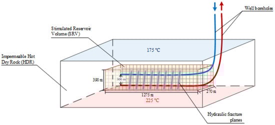
Figure 4.
Conceptual simulation model with highlighted well boreholes, SRV region, and hydraulic fractures.
2.2.2. Static Model
Geological model of the EGS reservoir was developed using the Petrel suite by Schlumberger. The first step was to create an overview model of the Milford area and locating the Utah FORGE site on the model’s surface. To achieve that, the surface data provided in GDR was used and next combined with the granitoid top surface location data, well locations and location of the two faults. The site location was constrained with the border polygon which allowed to load the faces of the isotherms 175 °C and 225 °C, located underneath the granitoid top. The model’s elements described above are presented in Figure 5, the faults are highlighted in pink and purple, and the bottom depth of the formation is not known. The model was limited by the polygon in a way that it would not exceed the actual FORGE site area and the Opal Mound fault that separates the approximate EGS location and the hydrothermal reservoir, which should not affect the reservoir properties and the simulation results [21].
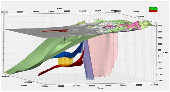
Figure 5.
Recreated model of the Milford area subsurface. Faults are represented by purple and pink planes. Yellow box is a representation of the EGS system location (the simulation model) and is limited from the top and bottom by two temperature profiles 175 (blue) and 225 °C (red) isotherms. Remaining surfaces represent respectively from the top: the Earth surface (with a highlighted exact location of the Utah FORGE site in red) and the top of granitoid formation in light green.
At this stage, injection (I1) and production well (P1) were added to the model. Both wells are horizontal and have their wellheads located in the location of the reference 58-32 well. The wells are positioned parallel to each other, and I1 is set above the P1 well. The injection well is located at depth 2302.41 m (TVD) and the production well lays 300 m below at depth of 2602.41 m (TVD). To reduce the computation time of the simulation, the model was further diminished and limited only to the near wellbore area in the granitoid formation. Grid properties, such as porosity and permeability, were fitted using random distribution, and their parameters are based on the granitoid data, which include the impact of naturally occurring faults [20,22,23]. The distribution of reservoir properties was conducted using the Sequential Gaussian simulation (SGS), which is a standard algorithm for modeling of the petrophysical parameters. The algorithm allows for estimating the distributions for a collection of points using the factorization of major probability of the data points and then data kriging for conditional distribution. It was chosen as it has proven to be efficient especially for irregular grids that include Local Grid Refinement [24]. As a result, a target simulation model containing 38,400 grid blocks, with the dimensions of 48 × 40 × 20 grid blocks in x, y and z directions, was received [2]. The porosity and vertical permeability distributions across the model are presented respectively in Figure 6 and Figure 7.
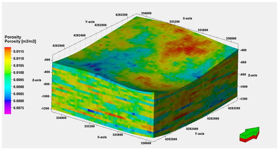
Figure 6.
Porosity distribution in the model’s grid [2].
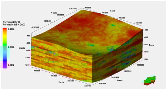
Figure 7.
Vertical permeability distribution in the model’s grid [2].
2.3. Hydraulic Fractures Design and Permeability Enhancement
Hydraulic fractures network was created using the Petrel’s fracture modeling tool, which is dedicated for generating DFNs of natural fractures. DFN modelling is an advanced approach for fracture modelling, of which different sets of fractures could be created. Each fracture is presented by a plane with specific parameters such as dip angle, dip azimuth and aperture, etc. The fracture model built by DFN approximates the real fracture distribution in plays. The petrophysical properties, e.g., porosity and permeability, can be calculated by upscaling the DFN model into cells in order to simulate the reservoir fluid flow. By adjusting the parameters for DFN distribution, a set of flat fracture planes was received, of which each one intersected both the injector and producer creating hydraulic fractured-like pathways for the working fluid, trying to follow a local stress distribution. Additionally, the fracture area is limited by the LGR region, which is in fact equivalent to the SRV. To receive more regular and uniform distribution of the fractures, the Fisher model was chosen. DFN distribution was modelled by application of a stochastic approach. Used parameters are presented in Table 1 below [2].

Table 1.
Geometrical properties of the fractures used as an input to Petrel’s DFNs modelling tool [2].
The main goal of introducing hydraulic fractures was an alteration of the permeability between the wells to create flow-through channels for the working fluid. Therefore, permeability properties of the generated DFN were incorporated into the global permeability matrix of the model. Figure 8 shows the distribution of permeability in the SRV range after the permeability alteration is included into the model [2].
Figure 8.
Permeability distribution in the SRV along the hydraulic fracture planes [2].
Fracture spacing used in this work is different than in most of the cases that can be found in the literature [4,15,23]. Since fluid flow in the modelled reservoir is downward and supported by the gravitational force, fracture spacing had to be increased to provide sufficient time for the working fluid to heat up and so the fractures are positioned 55 to 140 m from each other. Fractures distribution across the SRV and the corresponding change of the permeability are presented in Figure 9.
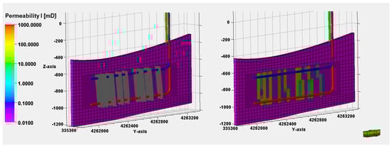
Figure 9.
Hydraulic fractures planes located in the model (left) and the permeability alteration along the fractures (right) [2].
Based on the permeability discrepancy across the model, two regions were created to separate the blocks affected by fracturing. This operation allowed full control of the properties of generated fractures and was used to determine model’s sensitivity to changes in the permeability. Initial permeability changes in the SRV were mostly visible only in the locations of fracture planes but also affected individual neighbour blocks of the grid. Created region covers all blocks that were touched by the alteration [2].
2.4. Reservoir Model Properties and Simulated Cases
2.4.1. Reservoir Properties
Reservoir properties of the simulation model correspond to the ones determined during phase 2 of the Utah FORGE project [19]. Based on laboratory and field measurements, and calibration of the official FORGE site earth model, parameters of the granitoid reservoir were specified. The calibration of the earth model mainly included applying the network of natural fractures as a DFN and upscaling the general reservoir properties to receive a final distribution of specific parameters such as porosity, permeability, and rock compaction [19,21,22]. The final reservoir parameters of the simulation model are presented in Table 2 [2].
Table 2.
Summary of the reservoir properties for the simulation model [2].
Thermal boundary conditions are determined by two isotherms, so the temperature varies from 175 °C to 225 °C and the average temperature of the reservoir is 200 °C. The initial reservoir pressure is constant for the whole model and equal to the pressure measured at the bottom of the reference 58-32 well at the end of the testing phase [19,22]. Additionally, specific heat capacity of the matrix in the last layer of the model was greatly increased to imitate the thermal energy influx from the lower layers of the granitic rock. The near-wellbore area, where the hydraulic fracturing effects were simulated, was refined with an LGR. Initial reservoir parameters of the LGR region are the same as the global properties of the model [2].
After introduction of the hydraulic fractures, initial permeability in the SRV region varied from 0.1 to 100 mD, while in most of the research, permeability of hydraulic fractures varies between 10 and 100,000 mD [23,25,26]. Based on the conclusions made by Nadmi et al. [23] and Guo et al. [26] and given the fact that, in case of this work, the propagation of the fractures is rather longitudinal than transverse, it was decided that the initial permeability values will be increased 10 times, and so the SRV permeability values for the reference case vary from 1 to 1000 mD. Reservoir properties of the SRV region for the base model are included in Table 3. Reservoir blocks outside the SRV are flagged as rock only, inactive blocks and do not take part in the fluid flow simulation [2].
Table 3.
Reservoir properties of the SRV region for the reference modelled case [2].
2.4.2. Reference Production Parameters and Simulated Cases
Reference parameters were modelled based on those used at the Soultz-sous-Forêts project because of the similar pressure and temperature conditions in the reservoir [19,27]. The main parameter that required adjustment was the injection/production flow rate, and the calibration run was performed with a flow rate initially set to 75 kg/s [28]. Because of the fact that, in the investigated well setup, the flow occurs downwards and is assisted by the gravitational force, the flow rate had to be significantly reduced. Greater flow affected the production temperature and, because of that, it has been gradually reduced until the satisfactory value of 25 kg/s was received. Higher flow rates are still included in the sensitivity analysis to demonstrate their effect on other parameters and the results. The operational properties summary for the reference is presented in Table 4 [2].
Table 4.
Summary of the production parameters for the reference simulation case [2].
One of the main objectives of this research was to analyse how the performance of the proposed system is affected by principal operational parameters; therefore, sensitivity to parameters such as injection rate, fluid injection temperature and production pressure has been checked. The goal was to check the influence of the fracture network’s permeability on the thermal efficiency and lifespan of the reservoir [29]. For the first set of simulations, the SRV permeability has been increased, so that the model allows for checking the impact of higher flow rates on the performance. The second set of simulations was completed using lower flow rate levels with optimized injection temperature and production pressure and with the original permeability distribution (Figure 8). Sets of operational properties for each of the simulation cases are presented in Table 5. For cases I–VI, the model with permeability enhancement of 10 times the initial value is used, while for cases VII, VIII & IX, original permeability is applied [2]. For all simulations, a commercial reservoir simulator Eclipse was used.
Table 5.
Summary of the simulation properties for each of the investigated cases [2].
3. Results and Discussion
In terms of reservoir engineering, there are two main parameters that define the performance of an EGS system. Those are the reservoir temperature decline and flow resistance. The flow resistance is determined mainly by the injection/production rate and, because of that, the rate should be possibly minimized. Temperature drawdown, however, is more complex to determine and control as it depends on various parameters, such as fracture distribution and conductivity but, in general, should be minimized as well [29]. The main indicator of the system’s efficiency in this analysis is the temperature decline curve; therefore, all results are presented in a form of Tpro vs. Time charts and temperature SRV profile for selected cases [2].
3.1. Reference Case Results
As we can see in Figure 10, the production temperature under reference conditions decreases from the initial value of 215 to 128 °C, which gives an almost 40% drop in the temperature from the start of the simulation. The stable stage of the production is very short and lasts not longer than 2.5 years; then, the declining stage occurs. The temperature chart is rather concave than convex, meaning that the conditions of the reference case will not provide an efficient level of production. As demonstrated in Figure 11, the temperature distribution indicates that four major fractures were created in the model through which large amounts of the injected fluid are flowing. Because of the unique well setup used in the project, high rates cause the working fluid to reach the production well too soon, which results in receiving part of the cold working fluid directly in the producer. The image shows that, after 10 years, the front line of cold water has already reached the production well in the locations of the two biggest fractures. This will obviously cause the gross power level to drop, due to production of a much cooler medium [2].
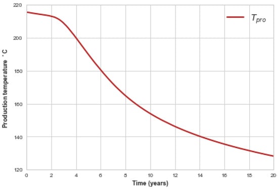
Figure 10.
Production temperature decline curve over 20 years of simulation (reference case) [2].
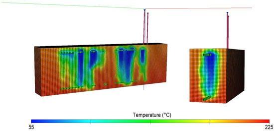
Figure 11.
Temperature distribution in the SRV after 10 years of simulation (reference case) [2].
3.2. Sensitivity Analysis Results
3.2.1. Sensitivity to Injection Temperature (Cases I & II)
Past research shows that lower injection temperatures may lead to higher efficiency but also cause a more rapid decrease in production temperature and lower energy production rates [23,29]. As shown in Figure 12, the lowest injection temperature caused a much bigger drop in the production temperature level over the simulation time. After 20 years, the temperature decreased to 106 °C, which is by about 51%, while in the case with the highest injection temperature, the temperature had decreased only by 35% from the initial value. This proves that the simulation results of the developed model correspond well with the literature information [2,23,29].
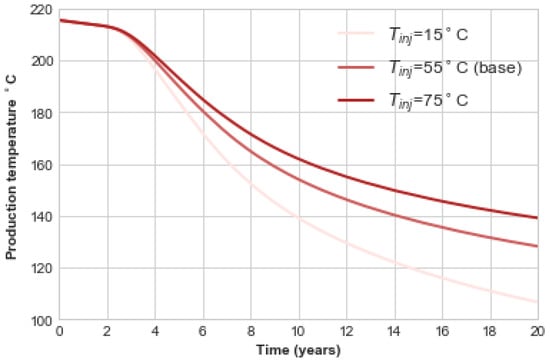
Figure 12.
Production temperature decline curve over 20 years of simulation for different injection temperatures [2].
3.2.2. Sensitivity to Injection/Production Flow Rate (Cases III & IV)
In this work, the production flow rate is almost equal to the injection rate which is a standard assumption for the EGS analysis, but fluid loss events might occur [23]. In the tested model, the loss is estimated to be less than 1% due to the fact that the flow occurs only in the SRV; therefore, fluid losses can be neglected and the assumption that is true [2].
As Figure 13 shows, the curve shape of the production temperature chart has slightly changed, meaning that the injection/production flow rate has a significant impact on the EGS performance. With the reduction of injection rate, duration of the stable stage of production has doubled, and the decline phase starts after 5–6 years of production. In addition, the decrease in the production temperature level is only by 14.4%, which, compared to the previous cases, is a significantly better result. Higher production rates seem to be ineffective, as the cool down of the reservoir happens much sooner, and the temperature decline level is concerning [2].
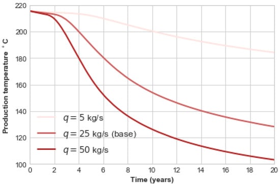
Figure 13.
Production temperature decline curve over 20 years of simulation for different production rates [2].
3.2.3. Sensitivity to Production Pressure (Cases V & VI)
Results of the simulations with different production pressures in the model had showed that overall performance of the EGS reservoir is insensitive to the level of reservoir pressure, which corresponds well with experiences from the past research [23,30]. Decreasing the production pressure will result in comparable drop in the injection pressure because of the fact that the pressure change only affects the SRV and not the whole reservoir. A similar effect can be usually observed in real-life, petrothermal EGS reservoirs [29,30]. Nevertheless, the model’s sensitivity to this parameter can be better understood using flow impedance as an indicator, which is defined as follows:
where Pinj and Ppro are the BHPs of the injector and producer, and q is the fluid production rate. It is a typical indicator for the EGS systems and represents the power required to provide one unit of production rate [15,27]. Changes in production pressure also affect the flow impedance. Flow impedance levels for cases V & VI are presented in Table 6. Looking at the results, we could have easily assumed that the decreases along with pressure but that is a case specific observation. Flow impedance is as low as is the pressure difference between the injection and production well [2,27].
Table 6.
Production pressure and flow impedance for sensitivity cases [2].
3.2.4. Cases VII, VIII and IX with Adjusted Permeability
After analysing the results from Cases I to VI, it is apparent that high flow rates for both injection and production cause the thermal efficiency of the whole system to decrease. This is a result of an unusual setup of the wells which accounts for the downward direction of the fluid flow that is additionally assisted by the presence of the gravitational force. Testing the effect of high flow rate levels required increasing the originally generated permeability, but, since the potentially optimal set of parameters will feature the flow rate levels below 20 kg/s, the permeability was again reduced to the original level to receive more uniform fluid distribution along the fractures. For all cases, with original permeability, the remaining parameters are applied at optimized levels; therefore, the injection temperature is equal to 55 °C, and the production pressure is 50 bar. Reducing the permeability is unequivocal to extending the time that the working fluid needs to flow through hydraulic fractures to the production well, which corresponds to prolonging the EGS system lifespan by maintaining the production temperature at a satisfactory level [2].
As demonstrated in Figure 14, production temperature for q = 5 kg/s is still above 200 °C after 20 years of production, which was not achieved in any of the previous cases. Compared to the results from case III where the temperature drop was at about 14.4%, here the decrease is as low as 6.3%. If we look at the shape of the curve, we can see that, for low flow rates, it is more flat, which indicates that the system is possibly more efficient than in the case of a strongly concave chart. Additionally, a stable stage of the production for cases VII and VIII is maintained for around 5–6 years, while, for case IX, it shortens to 4 years. Visualisation of how the production temperature looks in the SRV for case VIII (q = 10 kg/s) is presented in Figure 15. On the right, we can see that water saturation in the simulation blocks around the production well is high but at the same time temperature (left) holds at a satisfactory level. Compared to Figure 11, the distribution attained with lower flow rates is more uniform and at the same time favourable [2,4]. All in all, it is clear that lowering the injection rate will result in less significant temperature decline and prolonged EGS system lifetime.
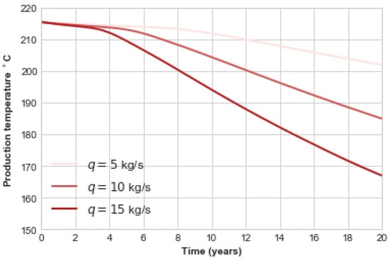
Figure 14.
Production temperature decline curve over 20 years of simulation for the scenarios with original permeability [2].
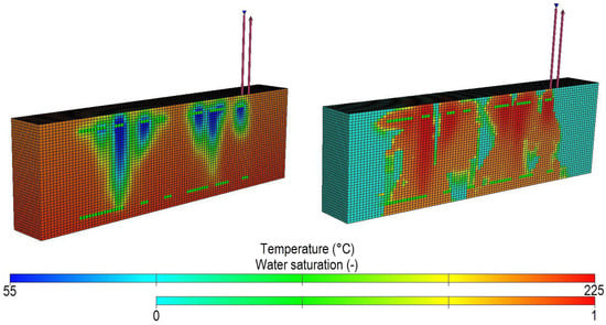
Figure 15.
Temperature distribution and water saturation in SRV region after 10 years for Case VIII [2].
By comparing the results of cases III (first run) and VIII (second run), the impact of fractures’ permeability can be analysed. Looking at Figure 13 and Figure 14, it is noticeable that, for q = 5 kg/s, the temperature at the end of simulation time is significantly lower when permeability had been increased. The difference in temperature drawdown over 20 years of simulation is of around 20 °C. According to the report published by MIT [3], the temperature decline should be no more than 10 °C compared to an average reservoir temperature [3,29]. If that is taken into consideration, fracture permeability has a great impact on the thermal efficiency of such system; hence, after the reduction of the permeability to original values, temperature decline for the lowest rate case was as low as 5 to 10 °C [2].
4. Conclusions
In this work, a novel EGS system development method, with horizontal wells, was proposed. With the help of common tools for reservoir modelling and simulation, a case study was performed which aimed to mimic the conditions at the actual EGS site. Using real-life data obtained from the open-source Utah FORGE project database, a fully coupled dynamic model with a discrete network of hydraulic fractures was created. To understand how primary production parameters would impact the performance of such a setup, a basic sensitivity study was presented. After an in-depth analysis of the results in terms of temperature decline over the EGS system lifespan and flow resistance in the SRV, the following conclusions were formulated [2]:
- (1)
- Production/injection rate is one of the most important parameters in EGS optimization and has the biggest impact on the temperature decline level in the reservoir.
- (2)
- The proposed setup of the wells requires using lower production and injection rates that should not exceed 20 kg/s. The optimal values of the flow rate for the suggested solution should vary from 5 to 10 kg/s.
- (3)
- Production and injection rates should be equal to maintain an efficient level of production. Inequality of these values might indicate that water loss events are occurring in the reservoir.
- (4)
- In the proposed solution, the flow rate of the working fluid also has an impact on the reservoir’s lifetime and duration of the stable stage of production and, for both, lower flow rates are favorable.
- (5)
- Injection temperature has an effect on the pace of temperature decrease in the reservoir. Lower injection temperatures will lead to a faster decline in the reservoir temperature and production of a low-temperature fluid in the early phase of reservoir development. At the same time, high injection temperature is unambiguous to higher maintenance costs.
- (6)
- The production and injection pressures have almost no effect on the production performance of the EGS.
- (7)
- The permeability of hydraulic fractures has a great impact on fluid distribution in the fracture network and the pace of temperature decline pace. Overall, the originally generated DFN’s permeability proved to be more effective.
- (8)
- In modelling of hydraulic fractures network using the Discrete Fracture Network technique, it is important to avoid the creation of big flow channels and aim for uniform distribution of the fluid in the whole fractured zone.
- (9)
- Reservoir simulation and modelling tools used in the oil and gas industry (Petrel and Eclipse by Schlumberger) prove to be effective in geothermal engineering [2].
Since this article only covers a preliminary analysis of the performance of such a solution and broadly covers the topic of reservoir behavior, there is still room for improvement and further research. The model could be improved by conducting a full analysis of the hydraulic fracturing process and attempting to model a design for the fracturing process. Analysis of the stresses around the wellbore and possible fracture propagation directions is also an interesting point for further research. The Utah FORGE data provide all necessary information for conducting such analysis on hydraulic fracturing conditions at the site. Further analysis of the system’s performance and both energy and economic analysis would be a beneficial extension to this research. Usually, the EGS development projects come with great investment risk; therefore, it is crucial to prepare a detailed economic model for such a solution to determine the project’s viability. In conclusion, a horizontal-well doublet with unique well positioning is likely to be applied as a method for a real-life Enhanced Geothermal System development.
Author Contributions
Conceptualization, J.K.; Methodology, J.K.; Validation, J.K.; Formal Analysis, J.K.; Writing—Original Draft Preparation, J.K.; Writing—Review and Editing, J.K. and D.J.; Supervision, D.J., P.W. All authors have read and agreed to the published version of the manuscript.
Funding
The paper was performed within the frame of AGH-UST statutory research Grant No. 16.16.190.779 Faculty of Drilling, Oil and Gas, Department of Petroleum Engineering.
Data Availability Statement
Not applicable.
Acknowledgments
We would like to acknowledge and thank all the contributors and the United States DOE FORGE Team for providing excellent quality data under open-license and their effort to engage the geothermal community to conduct research in the field of EGS systems.
Conflicts of Interest
The authors declare no conflict of interest.
Nomenclature
| BHP | Bottom Hole Pressure |
| DFN | Discrete Fracture Network |
| DOE | Department of Energy |
| EGS | Enhanced Geothermal System |
| EOS | Equations of State |
| FEHM | Finite Element Heat and Mass |
| FORGE | Frontier Observatory for Research in Geothermal Exploration |
| GDR | Geothermal Data Repository |
| HDR | Hot Dry Rocks |
| IR | Flow impedance (MPa/(kg/s)) |
| LGR | Local Grid Refinement |
| MINC | Multiple Interactive Continua |
| Pinj | Injection pressure (bar) |
| Ppro | Production pressure (bar) |
| q | Injection/ Production rate (kg/s) |
| qinj | Injection rate (kg/s) |
| qpro | Production rate (kg/s) |
| SGS | Sequential Gaussian Simulation |
| SRV | Stimulated Reservoir Volume |
| Tinj | Injection temperature ( °C) |
| Tpro | Production temperature ( °C) |
| TOUGH | Transport Of Unsaturated Groundwater and Heat |
| TVD | True Vertical Depth |
References
- Tester, J.; Anderson, B.; Batchelor, A.; Blackwell, D.; DiPippo, R.; Drake, E.; Garnish, J.; Livesay, B.; Moore, M.; Nichols, K.; et al. Impact of enhanced geothermal systems on US energy supply in the twenty-first century. Philos. Trans. Ser. A Math. Phys. Eng. Sci. 2007, 365, 1057–1094. [Google Scholar] [CrossRef] [PubMed]
- Kwasnik, J. Application of Horizontal Wells Technology in Petrothermal Reservoir Development. Master’s Thesis, AGH University of Science and Technology, Krakow, Poland, 2020. [Google Scholar]
- Batchelor, A.S.; Blackwell, D.D.; DiPippo, R.; Drake, E.M.; Garnish, J.; Livesay, B.; Moore, M.C.; Nichols, K.; Petty, S.; Toksoz, M.N.; et al. The Future of Geothermal Energy: Impact of Enhanced Geothermal Systems (EGS) on the United States in the 21st Century; Technical Report; Massachusetts Institute of Technology: Cambridge, MA, USA, 2006. [Google Scholar]
- Asai, P.; Panja, P.; Velasco, R.; McLennan, J.; Moore, J. Fluid flow distribution in fractures for a doublet system in Enhanced Geothermal Systems (EGS). Geothermics 2018, 75, 171–179. [Google Scholar] [CrossRef]
- Litvinenko, V. 115.1 Introduction. In Geomechanics and Geodynamics of Rock Masses, Volumes 1 and 2—Proceedings of the 2018 European Rock Mechanics Symposium (Eurock 2018, Saint Petersburg, Russia, 22–26 May 2018); CRC Press: Boca Raton, FL, USA, 2018; pp. 833–834. [Google Scholar]
- Aliyu, M.D. Hot Dry Rock Reservoir Modelling. Ph.D. Thesis, University of Greenwich, London, UK, 2018. [Google Scholar]
- Pruess, K. TOUGH2: A General-Purpose Numerical Simulator for Multiphase Fluid and Heat Flow; Technical Report; Lawrence Berkeley Laboratory, University of California: Berkeley, California, USA, 1991. [Google Scholar] [CrossRef]
- Sanyal, S.K.; Butler, S.J.; Swenson, D.; Hardeman, B. Review of the State-of-the-art of Numerical Simulation of Enhanced Geothermal Systems. In Proceedings of the World Geothermal Congress 2000, Kyushu-Tohoku, Japan, 28 May–10 June 2000. [Google Scholar]
- Warren, J.E.; Root, P.J. The Behavior of Naturally Fractured Reservoirs. Soc. Pet. Eng. J. 1963, 3, 245–255. [Google Scholar] [CrossRef]
- Pruess, K. Brief Guide to the MINC-Method for Modeling Flow and Transport in Fractured Media; Technical Report; Lawrence Berkeley Laboratory, University of California: Berkeley, California, USA, 1992. [Google Scholar] [CrossRef]
- Lei, Q.; Latham, J.P.; Tsang, C.F. The use of discrete fracture networks for modelling coupled geomechanical and hydrological behaviour of fractured rocks. Comput. Geotech. 2017, 85, 151–176. [Google Scholar] [CrossRef]
- Gong, F.; Guo, T.; Sun, W.; Li, Z.; Yang, B.; Chen, Y.; Qu, Z. Evaluation of geothermal energy extraction in Enhanced Geothermal System (EGS) with multiple fracturing horizontal wells (MFHW). Renew. Energy 2020, 151, 1339–1351. [Google Scholar] [CrossRef]
- Yao, J.; Zhang, X.; Sun, Z.; Huang, Z.; Liu, J.; Li, Y.; Xin, Y.; Yan, X.; Liu, W. Numerical simulation of the heat extraction in 3D-EGS with thermal-hydraulic-mechanical coupling method based on discrete fractures model. Geothermics 2018, 74, 19–34. [Google Scholar] [CrossRef]
- Zhang, H.; Sheng, J. Optimization of horizontal well fracturing in shale gas reservoir based on stimulated reservoir volume. J. Pet. Sci. Eng. 2020, 190, 107059. [Google Scholar] [CrossRef]
- Zeng, Y.C.; Su, Z.; Wu, N.Y. Numerical simulation of heat production potential from hot dry rock by water circulating through two horizontal wells at Desert Peak geothermal field. Energy 2013, 56, 92–107. [Google Scholar] [CrossRef]
- Lei, Z.; Zhang, Y.; Zhang, S.; Fu, L.; Hu, Z.; Yu, Z.; Li, L.; Zhou, J. Electricity generation from a three-horizontal-well enhanced geothermal system in the Qiabuqia geothermal field, China: Slickwater fracturing treatments for different reservoir scenarios. Renew. Energy 2020, 145, 65–83. [Google Scholar] [CrossRef]
- Cui, G.; Ren, S.; Zhang, L.; Ezekiel, J.; Enechukwu, C.; Wang, Y.; Zhang, R. Geothermal exploitation from hot dry rocks via recycling heat transmission fluid in a horizontal well. Energy 2017, 128, 366–377. [Google Scholar] [CrossRef]
- Xu, T.; Yuan, Y.; Jia, X.; Lei, Y.; Li, S.; Feng, B.; Hou, Z.; Jiang, Z. Prospects of power generation from an enhanced geothermal system by water circulation through two horizontal wells: A case study in the Gonghe Basin, Qinghai Province, China. Energy 2018, 148, 196–207. [Google Scholar] [CrossRef]
- Moore, J.; Nash, G.; Jones, C.; Kirby, S.; Kundsen, T.; Podgorney, R.; Allis, R.; McLennan, J.; Pankow, K.; Gwynn, M.; et al. Utah FORGE: Phase 2B Final Topical Report 2018; Technical Report; Energy & Geoscience Institute, University of Utah: Salt Lake City, UT, USA, 2018. [Google Scholar] [CrossRef]
- Open EI. Geothermal Data Repository. Available online: https://gdr.openei.org/ (accessed on 24 June 2020).
- Podgorney, R.; Finnila, A.; Mclennan, J.; Ghassemi, A.; Huang, H.; Forbes, B.; Elliott, J. A Framework for Modeling and Simulation of the Utah FORGE Site. In Proceedings of the 44th Workshop on Geothermal Reservoir Engineering, Stanford University, Stanford, CA, USA, 11–13 February 2019. [Google Scholar]
- Moore, J.; Jones, C.; Nash, G.; Erickson, B.; Miller, J.; Pankow, K.; Martin, T.; Simmons, S.; Skowron, G.; Hardwick, C.; et al. Utah FORGE: Phase 2C Final Topical Report— Section B: Results II. Dynamic Reservoir Modeling; Technical Report; Energy & Geoscience Institute, University of Utah: Salt Lake City, Utah, USA, 2019. [Google Scholar] [CrossRef]
- Nadimi, S.; Forbes, B.; Moore, J.; Podgorney, R.; McLennan, J. Utah FORGE: Hydrogeothermal modeling of a granitic based discrete fracture network. Geothermics 2020, 87, 101853. [Google Scholar] [CrossRef]
- Manchuk, J.G.; Deutsch, C.V. Implementation aspects of sequential Gaussian simulation on irregular points. Comput. Geosci. 2012, 16, 625–637. [Google Scholar] [CrossRef]
- Hofmann, H.; Babadagli, T.; Yoon, J.S.; Blöcher, G.; Zimmermann, G. A hybrid discrete/finite element modeling study of complex hydraulic fracture development for enhanced geothermal systems (EGS) in granitic basements. Geothermics 2016, 64, 362–381. [Google Scholar] [CrossRef]
- Guo, T.; Gong, F.; Wang, X.; Lin, Q.; Qu, Z.; Zhang, W. Performance of enhanced geothermal system (EGS) in fractured geothermal reservoirs with CO2 as working fluid. Appl. Therm. Eng. 2019, 152, 215–230. [Google Scholar] [CrossRef]
- Evans, K. Enhanced/engineered geothermal system: An introduction with overviews of deep systems built and circulated to date. In China Geothermal Development forum Beijing; China Geothermal Development Forum: Beijing, China, 2010. [Google Scholar]
- Lu, S.M. A global review of enhanced geothermal system (EGS). Renew. Sustain. Energy Rev. 2018, 81, 2902–2921. [Google Scholar] [CrossRef]
- Grant, M.A.; Bixley, P.F. Chapter 14—Well Stimulation and Engineered Geothermal Systems. In Geothermal Reservoir Engineering (Second Edition); Grant, M.A., Bixley, P.F., Eds.; Academic Press: Boston, MA, USA, 2011; pp. 269–281. [Google Scholar] [CrossRef]
- Pruess, K. On production behavior of enhanced geothermal systems with CO2 as working fluid. Energy Convers. Manag. 2008, 49, 1446–1454. [Google Scholar] [CrossRef]
Publisher’s Note: MDPI stays neutral with regard to jurisdictional claims in published maps and institutional affiliations. |
© 2022 by the authors. Licensee MDPI, Basel, Switzerland. This article is an open access article distributed under the terms and conditions of the Creative Commons Attribution (CC BY) license (https://creativecommons.org/licenses/by/4.0/).