
Optimal Design of Hybrid Renewable Energy Systems Considering Weather Forecasting Using Recurrent Neural Networks

Abstract
:1. Introduction
2. Background Framework
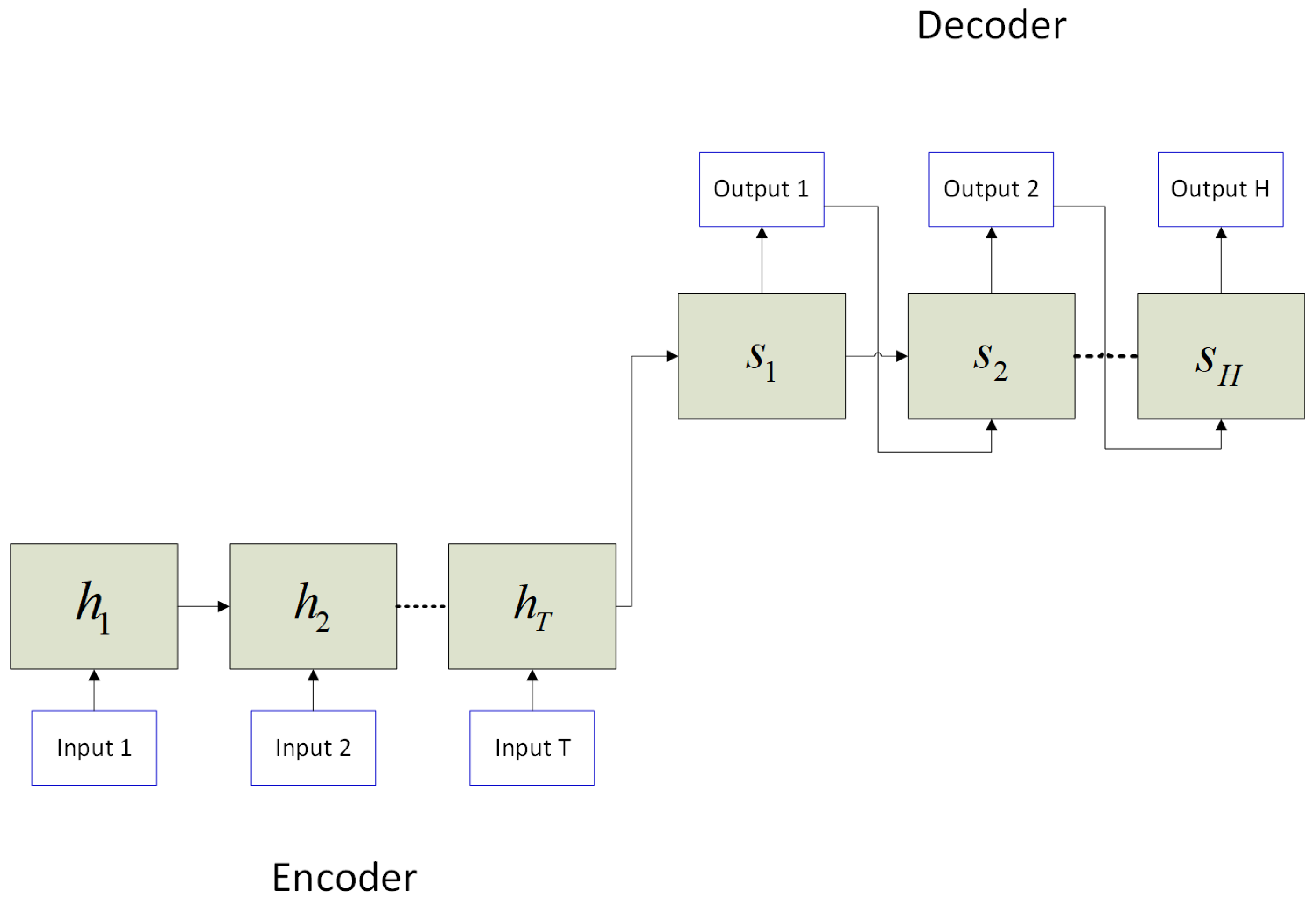
2.1. Recurrent Neural Networks
2.2. Benchmark Methods
2.3. Hierarchical Agglomerative Clustering
2.4. Optimization
3. NLP Model Formulation
3.1. Objective Function
3.1.1. Economic Dimension
3.1.2. Environmental Dimension
3.1.3. Social Dimension
3.2. Operational Constraints
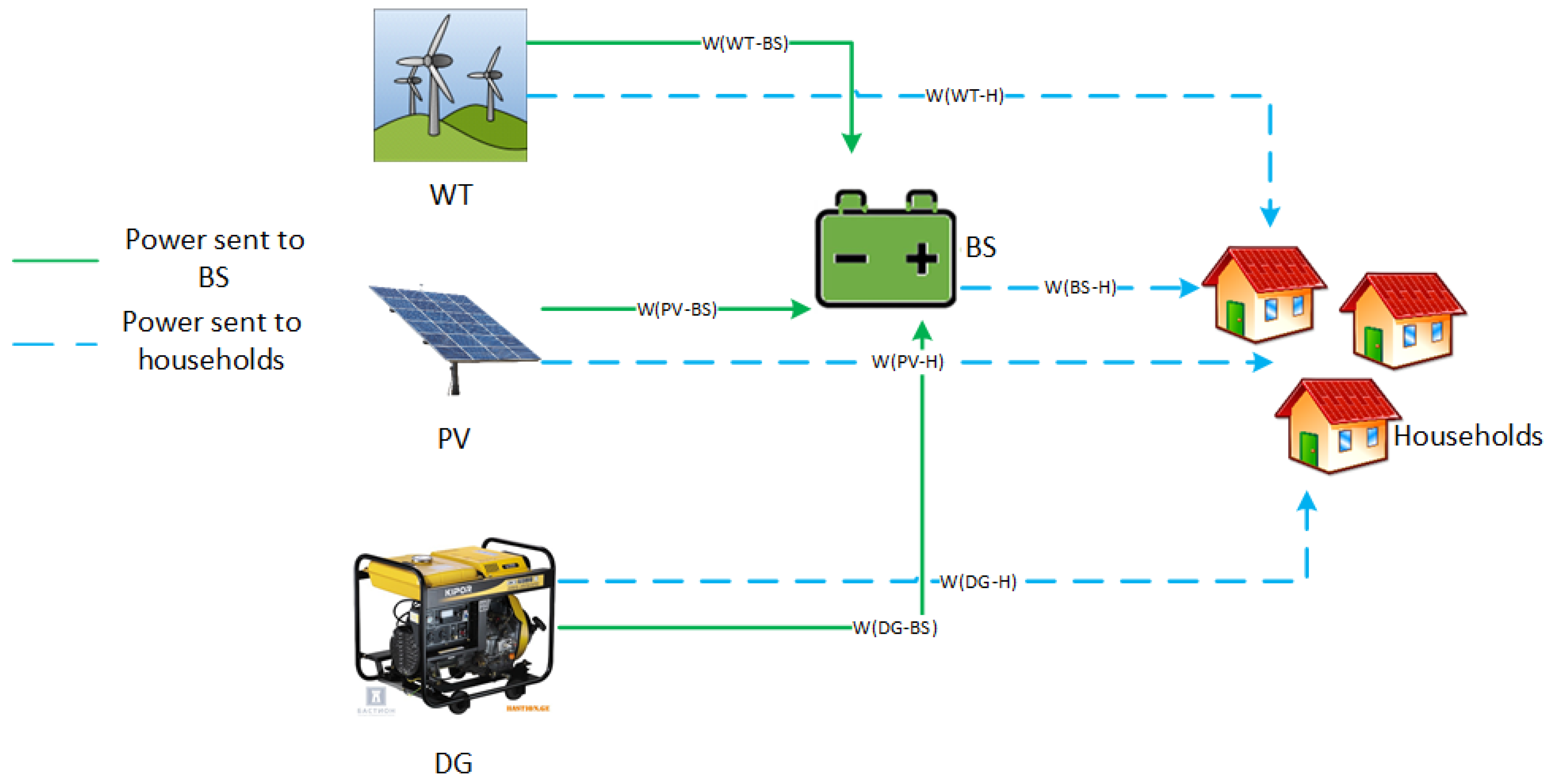
3.2.1. Power Generation
3.2.2. Energy Storage
3.2.3. Power Supply to Households
4. Case Study
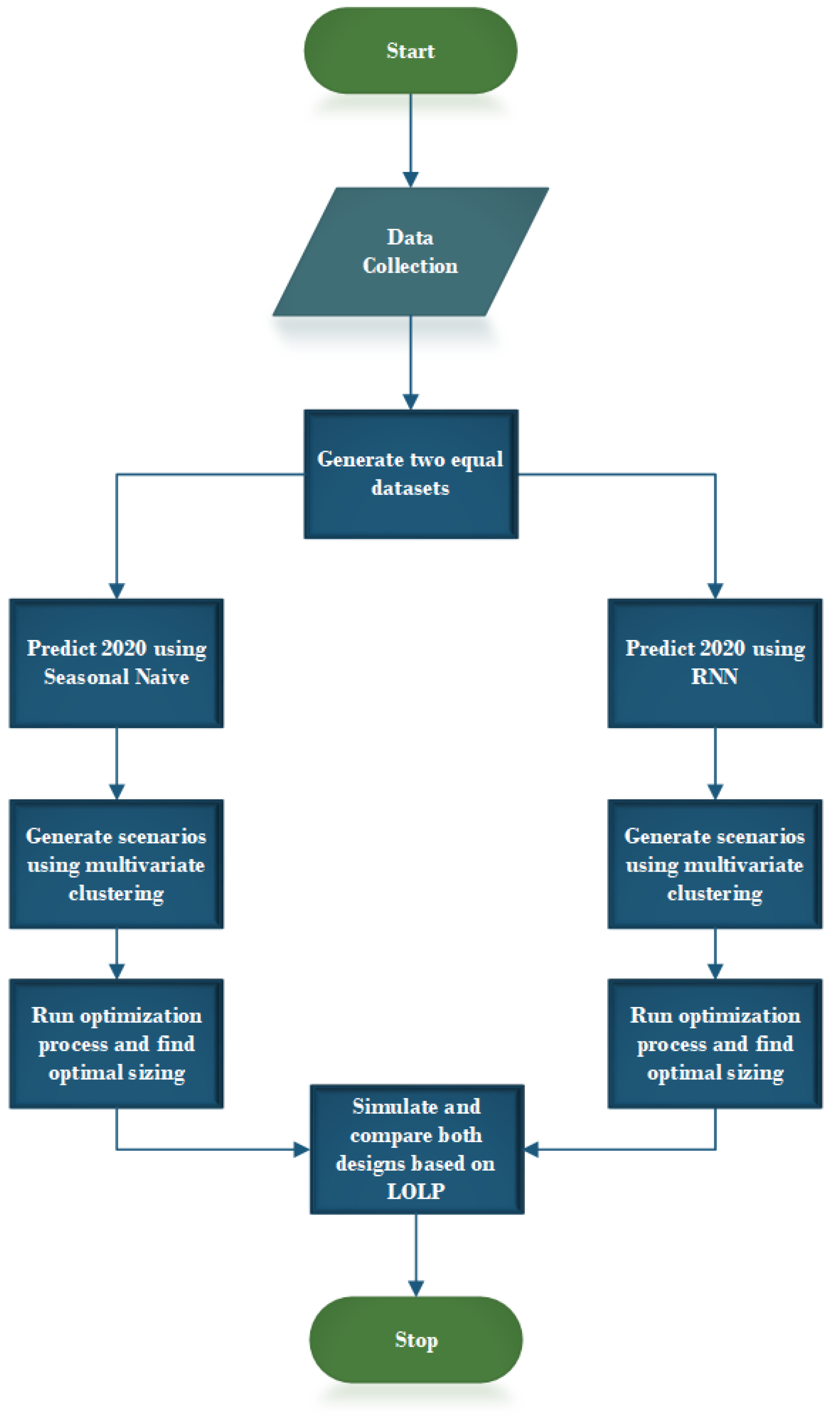
5. Methodology
6. Analysis of Results
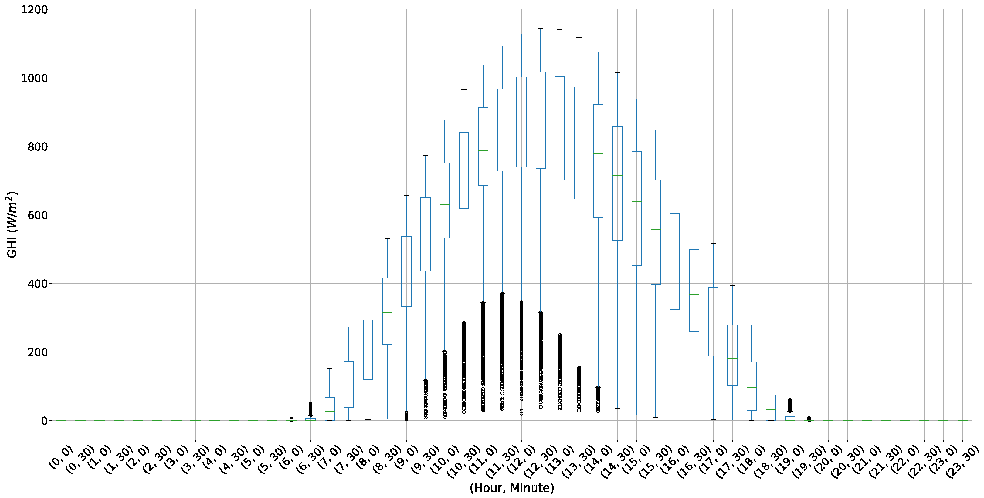
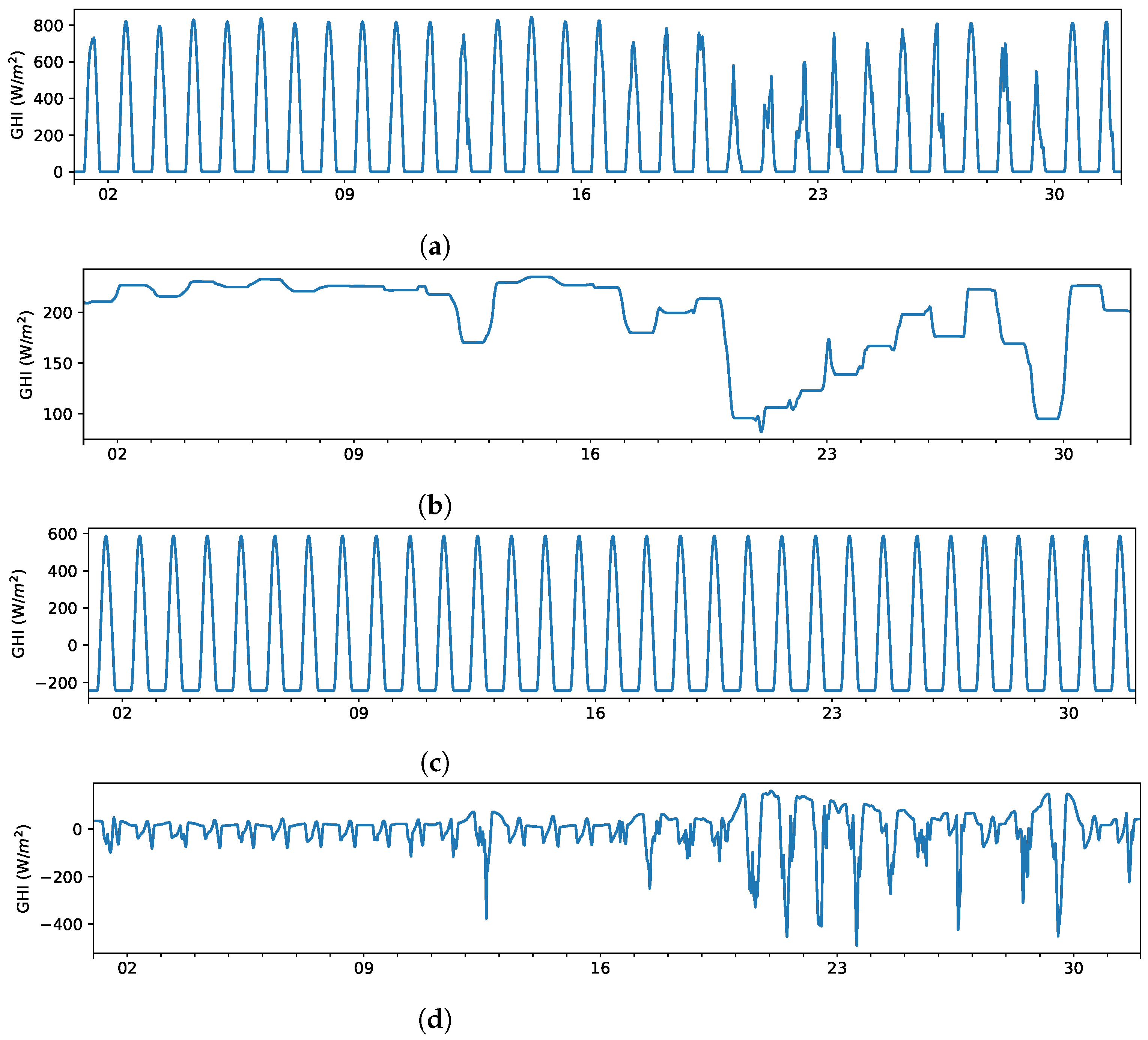
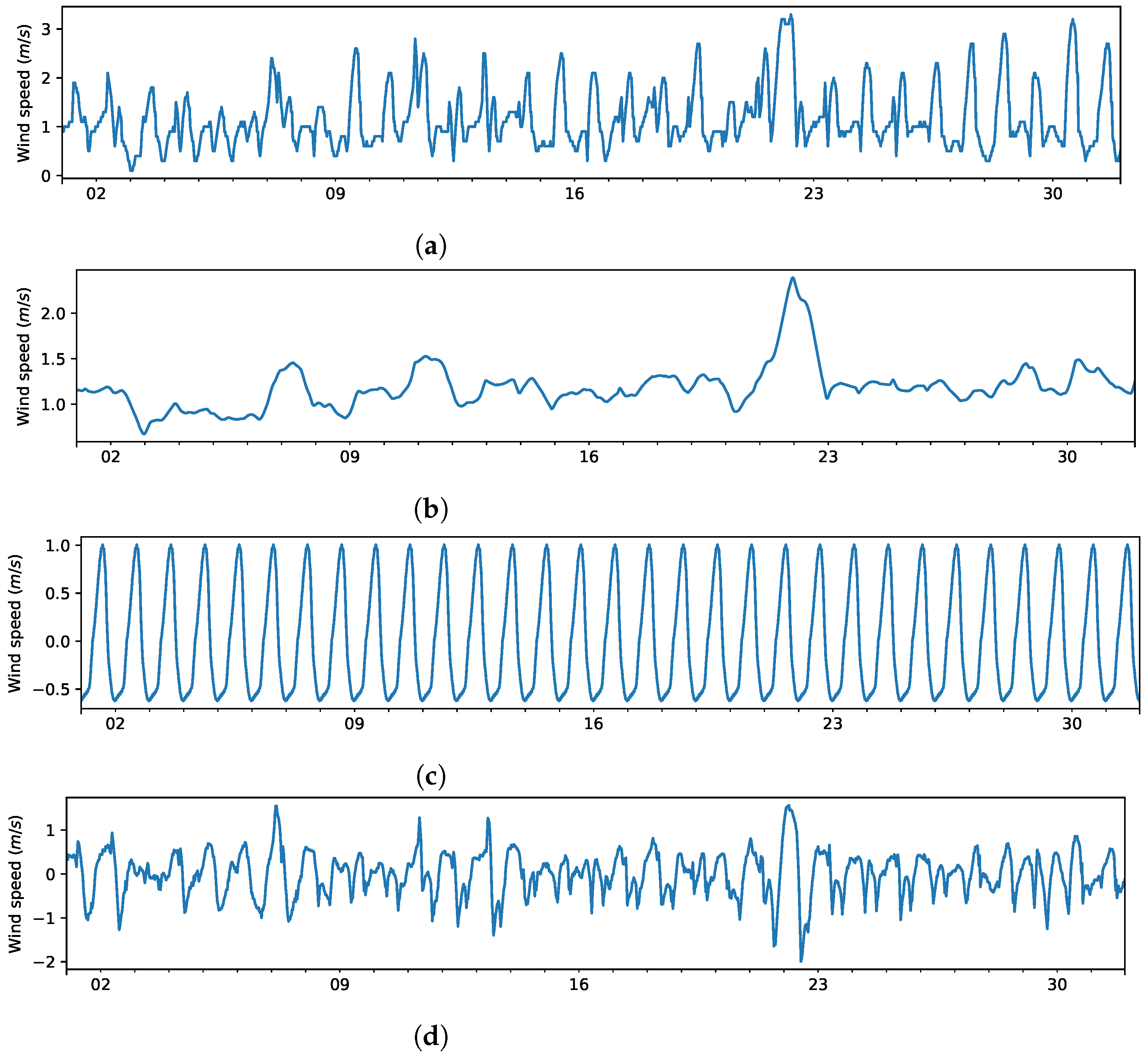
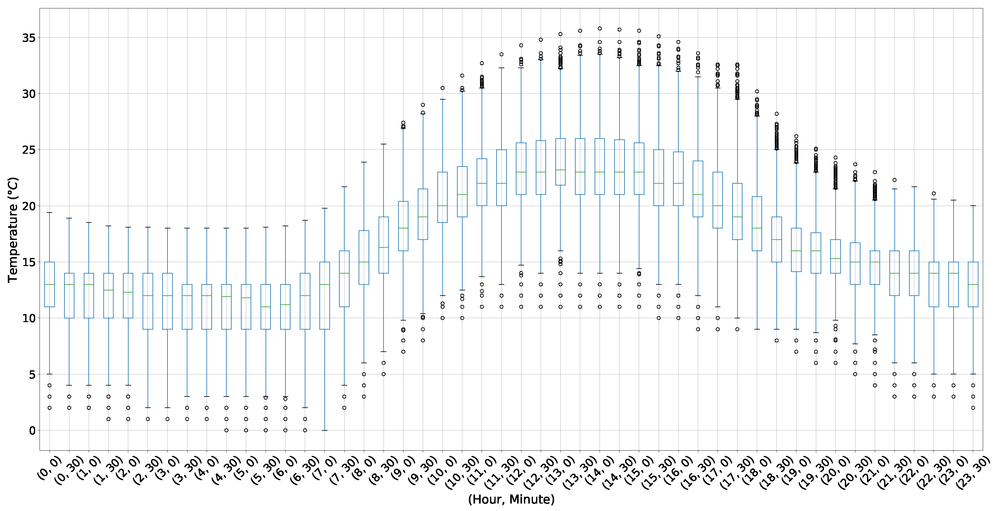
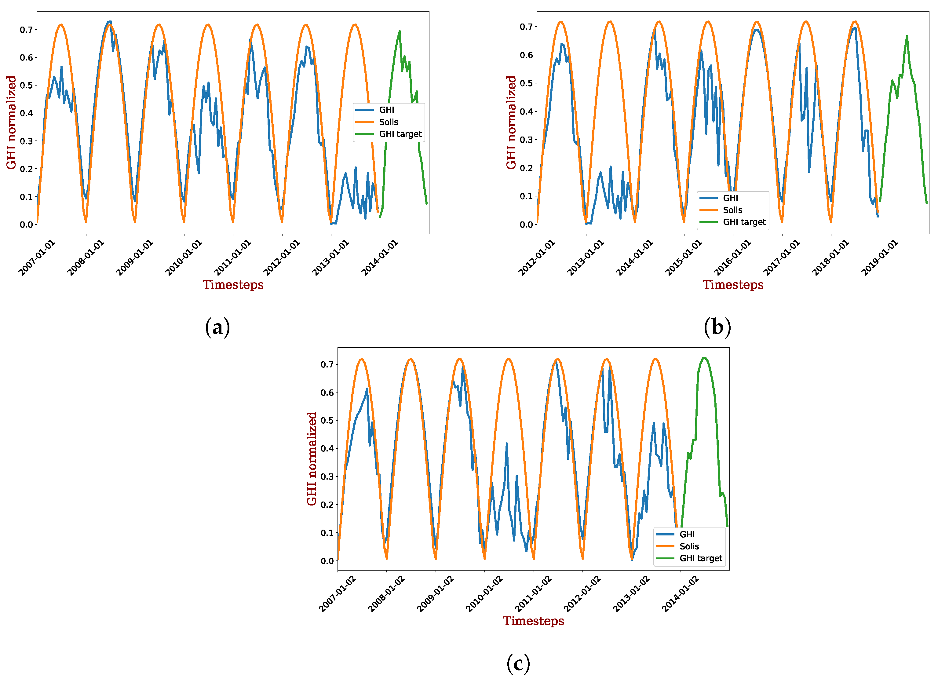
6.1. Data Exploration
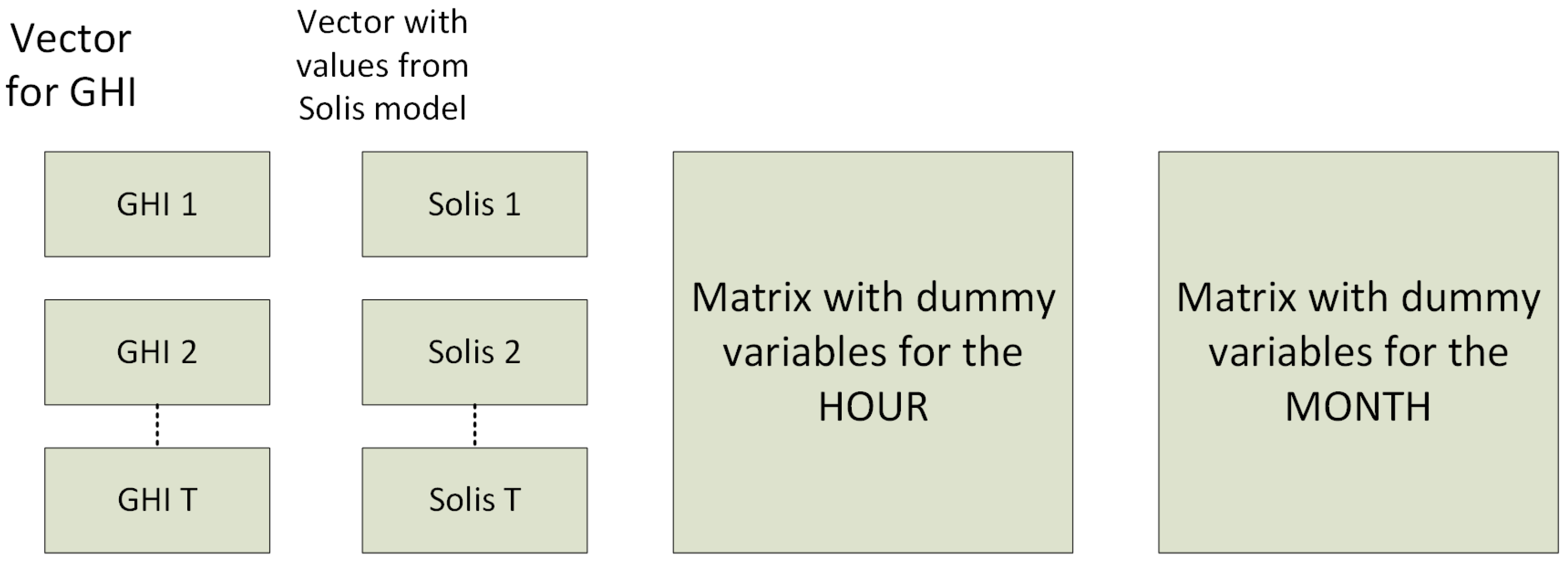
6.2. Data Preparation
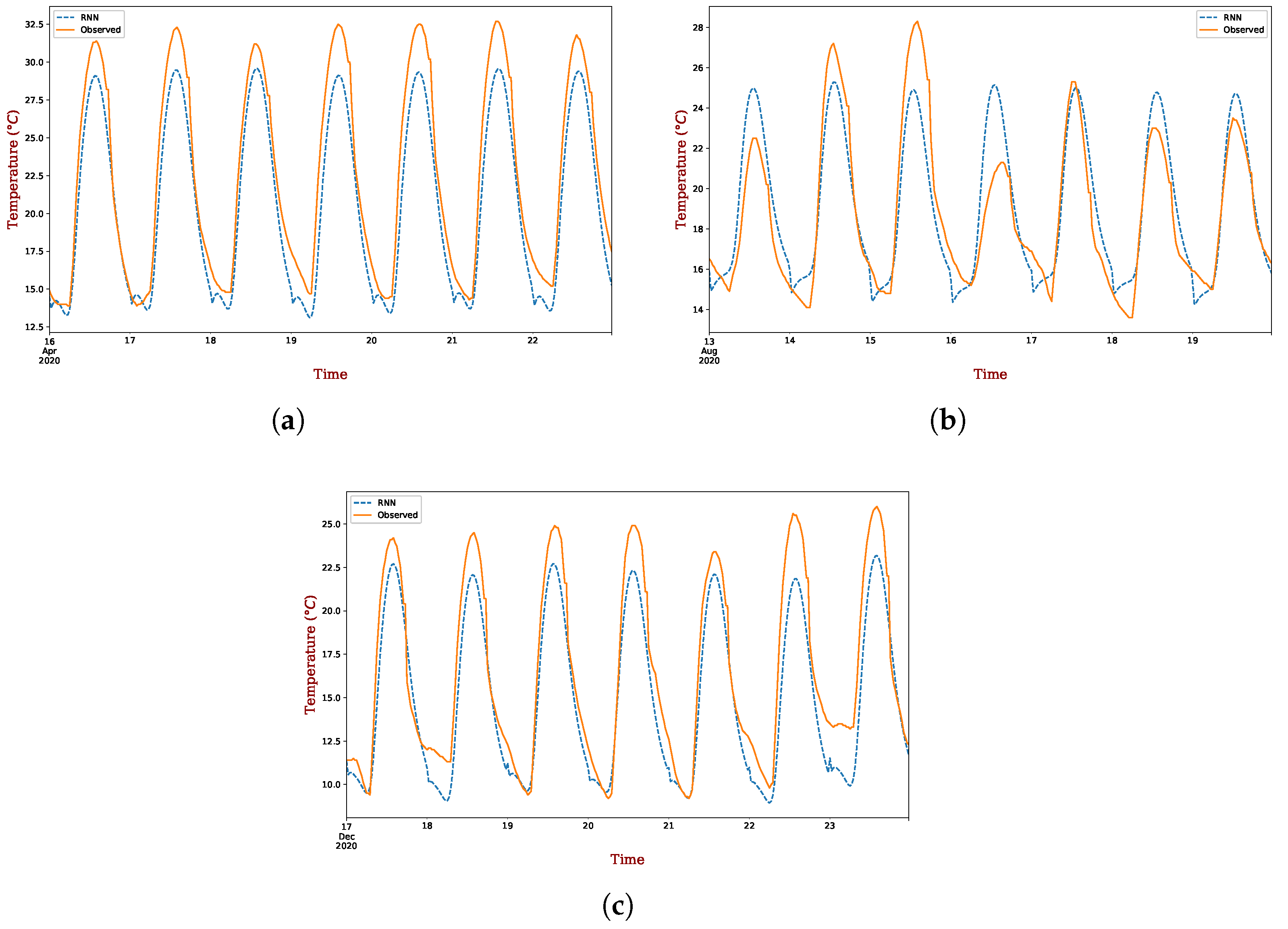
6.3. Evaluation
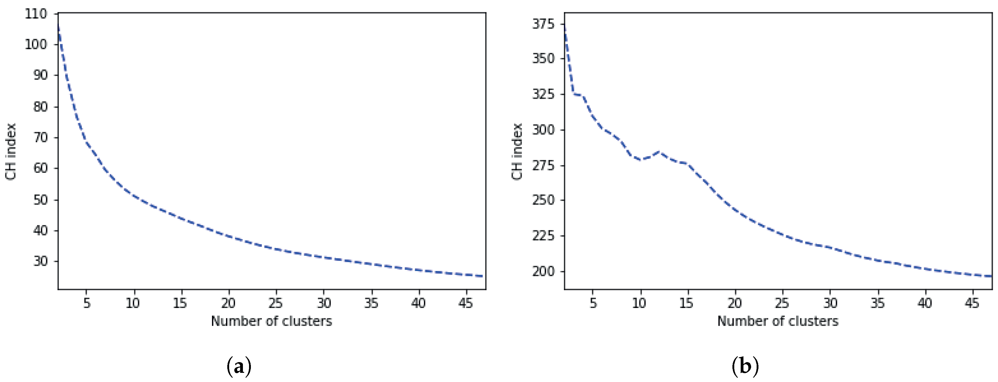
6.4. Hierarchical Clustering
6.5. Optimization Results
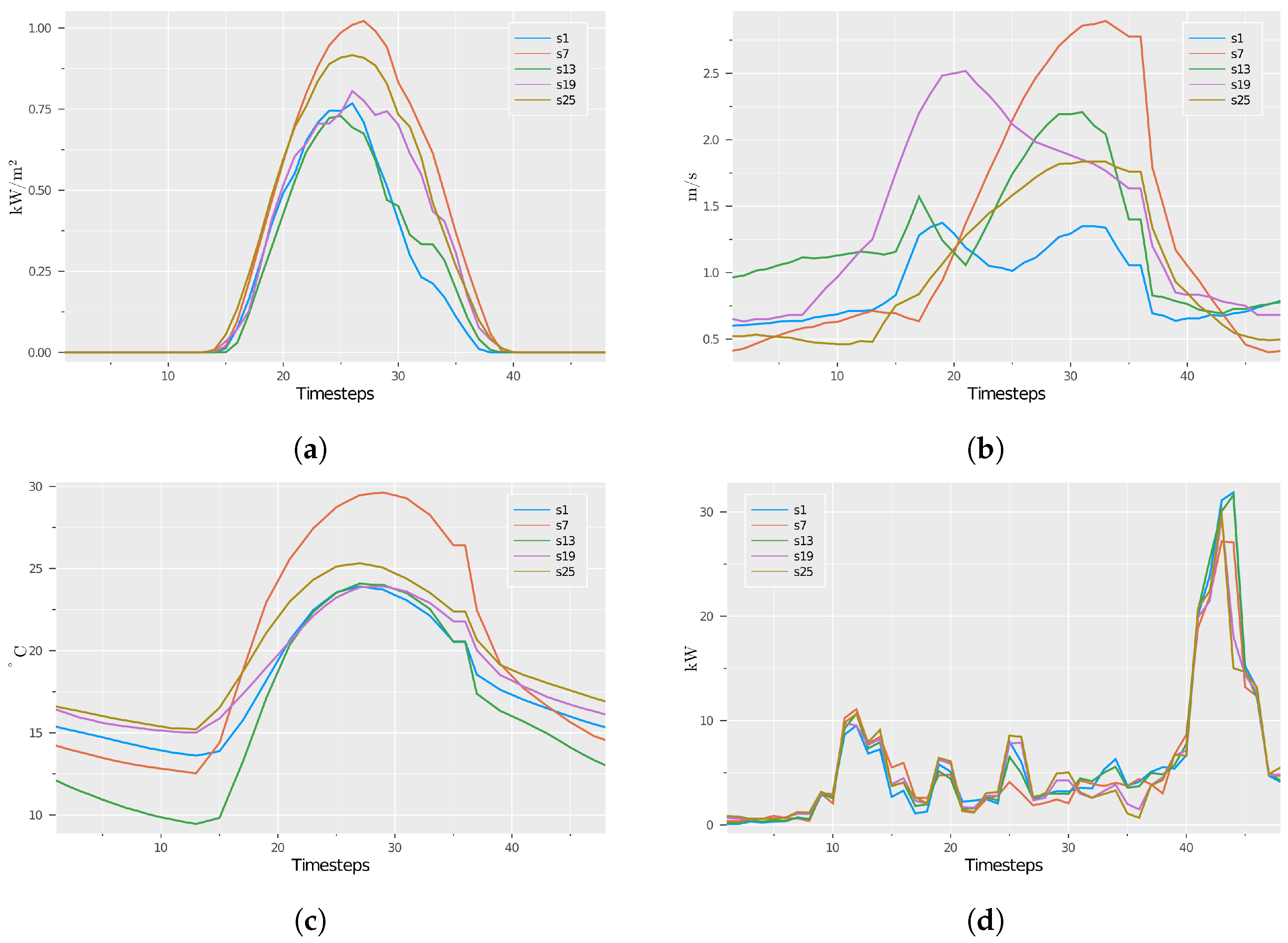
6.6. Simulation
7. Conclusions and Future Work
Author Contributions
Funding
Institutional Review Board Statement
Informed Consent Statement
Data Availability Statement
Acknowledgments
Conflicts of Interest
Abbreviations
| Sets | ||
| Symbol | Description | Units |
| t— | Time | 30 min period |
| s— | Scenario | Period of days |
| — | Power generation technologies | |
| Acronyms | ||
| Symbol | Description | Units |
| amb | Ambient conditions | |
| BS | Battery system | |
| H | Housing—households | |
| INV | Inverter | |
| LB | Lower bound | |
| MAX | Maximum | |
| MIN | Minimum | |
| NLP | Nonlinear programming | |
| O&M, OM | Operation and maintenance | |
| PV | Photovoltaic system | |
| SO | Social objective | |
| TAC | Total annual cost | |
| UB | Upper bound | |
| W | Electricity | |
| WT | Wind turbine | |
| Variables | ||
| A | Area allocated for a unit | m2 |
| Cost | $ | |
| Capital cost | $ | |
| E | Energy | kWh |
| f | Objective function | |
| Operation and maintenance cost | $ | |
| State of charge | ||
| Social objective | ||
| T | Temperature | °C |
| W | Electric flux | kW |
| Total annual cost | $/year | |
| Efficiency | ||
| Operative function | ||
| Parameter | ||
| Annualization factor | $ | |
| Security factor | ||
| Solar irradiance | kW/m2 | |
| Temperature coefficient of the PV system | ||
| Unit cost | $/kWh, $/kW | |
| Factor for land usage | kW/m2, kWh/m2 | |
| Duration of a time period t | h | |
| Variable cost | $/kW, $/m2, $/kWh | |
| Fixed cost | $ | |
| Density | kg/m3 | |
| Duration of each scenario s | days | |
| Wind speed | m/s | |
| Abbreviation | ||
| NL | Nonlinear | |
| LSTM | Long short-term memory | |
| FFNN | Feedforward neural network | |
| RNN | Recurrent neural network | |
| HRES | Hybrid renewable energy system |
References
- Ameur, H.B.; Han, X.; Liu, Z.; Peillex, J. When did the global warming start? A new baseline for carbon budgeting. Econ. Model. 2022, 116, 106005. [Google Scholar] [CrossRef]
- Lu, Z.Q.; Wu, C.G.; Wu, N.Y.; Lu, H.L.; Wang, T.; Xiao, R.; Liu, H.; Wu, X.H. Change trend of natural gas hydrates in permafrost on the Qinghai-Tibet Plateau (1960–2050) under the background of global warming and their impacts on carbon emissions. China Geol. 2022, 5, 475–509. [Google Scholar]
- IEA. World Energy Outlook 2020. Available online: https://www.iea.org/reports/world-energy-outlook-2020 (accessed on 1 October 2021).
- Kahwash, F.; Barakat, B.; Taha, A.; Abbasi, Q.H.; Imran, M.A. Optimising Electrical Power Supply Sustainability Using a Grid-Connected Hybrid Renewable Energy System—An NHS Hospital Case Study. Energies 2021, 14, 7084. [Google Scholar] [CrossRef]
- Lim, B.; Hong, K.; Yoon, J.; Chang, J.I.; Cheong, I. Pitfalls of the eu’s carbon border adjustment mechanism. Energies 2021, 14, 7303. [Google Scholar] [CrossRef]
- SENER. Reporte de Avance de Energías Limpias Primer Semestre 2018; SENER: Getxo, Spain, 2018; p. 21. [Google Scholar]
- Erdinc, O. Optimization in Renewable Energy Systems: Recent Perspectives; Butterworth-Heinemann: Oxford, UK, 2017. [Google Scholar]
- Bank, W. Sustainable Energy for all Database. 2017. Available online: https://data.worldbank.org/indicator/EG.ELC.ACCS.RU.ZS (accessed on 27 April 2020).
- Ferrer-Martí, L.; Domenech, B.; García-Villoria, A.; Pastor, R. A MILP model to design hybrid wind-photovoltaic isolated rural electrification projects in developing countries. Eur. J. Oper. Res. 2013, 226, 293–300. [Google Scholar] [CrossRef]
- Eriksson, E.; Gray, E.M. Optimization of renewable hybrid energy systems–A multi-objective approach. Renew. Energy 2019, 133, 971–999. [Google Scholar] [CrossRef]
- Emad, D.; El-Hameed, M.; Yousef, M.; El-Fergany, A. Computational methods for optimal planning of hybrid renewable microgrids: A comprehensive review and challenges. Arch. Comput. Methods Eng. 2019, 27, 1297–1319. [Google Scholar] [CrossRef]
- Al-Falahi, M.D.; Jayasinghe, S.; Enshaei, H. A review on recent size optimization methodologies for standalone solar and wind hybrid renewable energy system. Energy Convers. Manag. 2017, 143, 252–274. [Google Scholar] [CrossRef]
- Kusakana, K.; Vermaak, H.; Numbi, B. Optimal sizing of a hybrid renewable energy plant using linear programming. In Proceedings of the IEEE Power and Energy Society Conference and Exposition in Africa: Intelligent Grid Integration of Renewable Energy Resources (PowerAfrica), Bari, Italy, 7–10 September 2021; IEEE: Piscataway, NJ, USA, 2012; pp. 1–5. [Google Scholar]
- Domenech, B.; Ranaboldo, M.; Ferrer-Martí, L.; Pastor, R.; Flynn, D. Local and regional microgrid models to optimise the design of isolated electrification projects. Renew. Energy 2018, 119, 795–808. [Google Scholar] [CrossRef]
- Khatod, D.K.; Pant, V.; Sharma, J. Analytical approach for well-being assessment of small autonomous power systems with solar and wind energy sources. IEEE Trans. Energy Convers. 2009, 25, 535–545. [Google Scholar] [CrossRef]
- Luna-Rubio, R.; Trejo-Perea, M.; Vargas-Vázquez, D.; Ríos-Moreno, G. Optimal sizing of renewable hybrids energy systems: A review of methodologies. Sol. Energy 2012, 86, 1077–1088. [Google Scholar] [CrossRef]
- Nadjemi, O.; Nacer, T.; Hamidat, A.; Salhi, H. Optimal hybrid PV/wind energy system sizing: Application of cuckoo search algorithm for Algerian dairy farms. Renew. Sustain. Energy Rev. 2017, 70, 1352–1365. [Google Scholar] [CrossRef]
- Suman, G.K.; Guerrero, J.M.; Roy, O.P. Optimisation of solar/wind/bio-generator/diesel/battery based microgrids for rural areas: A PSO-GWO approach. Sustain. Cities Soc. 2021, 67, 102723. [Google Scholar] [CrossRef]
- Bahramara, S.; Moghaddam, M.P.; Haghifam, M. Optimal planning of hybrid renewable energy systems using HOMER: A review. Renew. Sustain. Energy Rev. 2016, 62, 609–620. [Google Scholar] [CrossRef]
- Lambert, T.W.; Hittle, D. Optimization of autonomous village electrification systems by simulated annealing. Sol. Energy 2000, 68, 121–132. [Google Scholar] [CrossRef]
- Das, B.K.; Al-Abdeli, Y.M.; Kothapalli, G. Optimisation of stand-alone hybrid energy systems supplemented by combustion-based prime movers. Appl. Energy 2017, 196, 18–33. [Google Scholar] [CrossRef]
- Lan, H.; Wen, S.; Hong, Y.Y.; David, C.Y.; Zhang, L. Optimal sizing of hybrid PV/diesel/battery in ship power system. Appl. Energy 2015, 158, 26–34. [Google Scholar] [CrossRef] [Green Version]
- Abd el Motaleb, A.M.; Bekdache, S.K.; Barrios, L.A. Optimal sizing for a hybrid power system with wind/energy storage based in stochastic environment. Renew. Sustain. Energy Rev. 2016, 59, 1149–1158. [Google Scholar] [CrossRef]
- Iqbal, M.M.; Sajjad, I.A.; Khan, M.F.N.; Liaqat, R.; Shah, M.A.; Muqeet, H.A. Energy management in smart homes with pv generation, energy storage and home to grid energy exchange. In Proceedings of the 2019 International Conference on Electrical, Communication, and Computer Engineering (ICECCE), Swat, Pakistan, 24–25 July 2019; IEEE: Piscataway, NJ, USA, 2019; pp. 1–7. [Google Scholar]
- Rasheed, M.B.; Javaid, N.; Ahmad, A.; Jamil, M.; Khan, Z.A.; Qasim, U.; Alrajeh, N. Energy optimization in smart homes using customer preference and dynamic pricing. Energies 2016, 9, 593. [Google Scholar] [CrossRef] [Green Version]
- Nasir, T.; Raza, S.; Abrar, M.; Muqeet, H.A.; Jamil, H.; Qayyum, F.; Cheikhrouhou, O.; Alassery, F.; Hamam, H. Optimal scheduling of campus microgrid considering the electric vehicle integration in smart grid. Sensors 2021, 21, 7133. [Google Scholar] [CrossRef]
- Muqeet, H.A.; Munir, H.M.; Javed, H.; Shahzad, M.; Jamil, M.; Guerrero, J.M. An energy management system of campus microgrids: State-of-the-art and future challenges. Energies 2021, 14, 6525. [Google Scholar] [CrossRef]
- Muqeet, H.A.; Javed, H.; Akhter, M.N.; Shahzad, M.; Munir, H.M.; Nadeem, M.U.; Bukhari, S.S.H.; Huba, M. Sustainable Solutions for Advanced Energy Management System of Campus Microgrids: Model Opportunities and Future Challenges. Sensors 2022, 22, 2345. [Google Scholar] [CrossRef]
- Fei, L.; Shahzad, M.; Abbas, F.; Muqeet, H.A.; Hussain, M.M.; Bin, L. Optimal Energy Management System of IoT-Enabled Large Building Considering Electric Vehicle Scheduling, Distributed Resources, and Demand Response Schemes. Sensors 2022, 22, 7448. [Google Scholar] [CrossRef] [PubMed]
- Balouch, S.; Abrar, M.; Abdul Muqeet, H.; Shahzad, M.; Jamil, H.; Hamdi, M.; Malik, A.; Hamam, H. Optimal Scheduling of Demand Side Load Management of Smart Grid Considering Energy Efficiency. Front. Energy Res. 2022, 10, 861571. [Google Scholar]
- Kamjoo, A.; Maheri, A.; Dizqah, A.M.; Putrus, G.A. Multi-objective design under uncertainties of hybrid renewable energy system using NSGA-II and chance constrained programming. Int. J. Electr. Power Energy Syst. 2016, 74, 187–194. [Google Scholar] [CrossRef]
- Hosseini, S.M.; Carli, R.; Dotoli, M. Robust optimal energy management of a residential microgrid under uncertainties on demand and renewable power generation. IEEE Trans. Autom. Sci. Eng. 2020, 18, 618–637. [Google Scholar] [CrossRef]
- Hosseini, S.M.; Carli, R.; Dotoli, M. Robust energy scheduling of interconnected smart homes with shared energy storage under quadratic pricing. In Proceedings of the 2019 IEEE 15th International Conference on Automation Science and Engineering (CASE), Vancouver, BC, Canada, 22–26 August 2019; IEEE: Piscataway, NJ, USA, 2019; pp. 966–971. [Google Scholar]
- Zakaria, A.; Ismail, F.B.; Lipu, M.H.; Hannan, M.A. Uncertainty models for stochastic optimization in renewable energy applications. Renew. Energy 2020, 145, 1543–1571. [Google Scholar] [CrossRef]
- Fuentes-Corté, L.F.; Ortega-Quintanilla, M.; Flores-Tlacuahuac, A. Water–Energy Off-Grid Systems Design Using a Dominant Stakeholder Approach. ACS Sustain. Chem. Eng. 2019, 7, 8554–8578. [Google Scholar] [CrossRef]
- Fuentes-Cortés, L.F.; Ponce-Ortega, J.M. Optimal design of energy and water supply systems for low-income communities involving multiple-objectives. Energy Convers. Manag. 2017, 151, 43–52. [Google Scholar] [CrossRef]
- Singla, P.; Duhan, M.; Saroha, S. A comprehensive review and analysis of solar forecasting techniques. Front. Energy 2021, 16, 187–223. [Google Scholar] [CrossRef]
- Aslam, M.; Seung, K.H.; Lee, S.J.; Lee, J.M.; Hong, S.; Lee, E.H. Long-term Solar Radiation Forecasting using a Deep Learning Approach-GRUs. In Proceedings of the 2019 IEEE 8th International Conference on Advanced Power System Automation and Protection (APAP), Xi’an, China, 21–24 October 2019; IEEE: Piscataway, NJ, USA, 2019; pp. 917–920. [Google Scholar]
- Kumar, N.M.; Subathra, M. Three years ahead solar irradiance forecasting to quantify degradation influenced energy potentials from thin film (a-Si) photovoltaic system. Results Phys. 2019, 12, 701–703. [Google Scholar] [CrossRef]
- Zhang, W.; Maleki, A.; Rosen, M.A. A heuristic-based approach for optimizing a small independent solar and wind hybrid power scheme incorporating load forecasting. J. Clean. Prod. 2019, 241, 117920. [Google Scholar] [CrossRef]
- Zhang, W.; Maleki, A.; Rosen, M.A.; Liu, J. Sizing a stand-alone solar-wind-hydrogen energy system using weather forecasting and a hybrid search optimization algorithm. Energy Convers. Manag. 2019, 180, 609–621. [Google Scholar] [CrossRef]
- Gupta, R.; Kumar, R.; Bansal, A.K. BBO-based small autonomous hybrid power system optimization incorporating wind speed and solar radiation forecasting. Renew. Sustain. Energy Rev. 2015, 41, 1366–1375. [Google Scholar] [CrossRef]
- Maleki, A.; Khajeh, M.G.; Rosen, M.A. Weather forecasting for optimization of a hybrid solar-wind–powered reverse osmosis water desalination system using a novel optimizer approach. Energy 2016, 114, 1120–1134. [Google Scholar] [CrossRef]
- Smyl, S. A hybrid method of exponential smoothing and recurrent neural networks for time series forecasting. Int. J. Forecast. 2020, 36, 75–85. [Google Scholar] [CrossRef]
- Hewamalage, H.; Bergmeir, C.; Bandara, K. Recurrent neural networks for time series forecasting: Current status and future directions. Int. J. Forecast. 2021, 37, 388–427. [Google Scholar] [CrossRef]
- Müllner, D. Modern hierarchical, agglomerative clustering algorithms. arXiv 2011, arXiv:1109.2378. [Google Scholar]
- Otto, K.N. Product Design: Techniques in Reverse Engineering and new Product Development; Prentice Hall: Hoboken, NJ, USA, 2003. [Google Scholar]
- Askarzadeh, A. Optimisation of solar and wind energy systems: A survey. Int. J. Ambient. Energy 2017, 38, 653–662. [Google Scholar] [CrossRef]
- Čepin, M. Assessment of Power System Reliability: Methods and Applications; Springer Science & Business Media: Berlin/Heidelberg, Germany, 2011. [Google Scholar]
- Maleki, A.; Pourfayaz, F. Optimal sizing of autonomous hybrid photovoltaic/wind/battery power system with LPSP technology by using evolutionary algorithms. Sol. Energy 2015, 115, 471–483. [Google Scholar] [CrossRef]
- INEGI (National Institute of Statistics). Anuario Estadìstico y Geogràfico de Michoacàn de Ocampo; INEGI (National Institute of Statistics): Aguascalientes, Mexico, 2017.
- IEA (International Energy Agency) National Solar Radiation Database. 2021. Available online: https://nsrdb.nrel.gov/ (accessed on 13 November 2022).
- Sengupta, M.; Xie, Y.; Lopez, A.; Habte, A.; Maclaurin, G.; Shelby, J. The national solar radiation data base (NSRDB). Renew. Sustain. Energy Rev. 2018, 89, 51–60. [Google Scholar] [CrossRef]
- INEGI (Instituto Nacional de EstadÍ y Stica Geografía). Anuario Estadístico y Geográfico de Michoacán de Ocampo 2017; Instituto Nacional de EstadÍ y Stica Geografía: Aguascalientes, Mexico, 2018; Volume 10, p. 132. [CrossRef] [Green Version]
- IRENA (International Renewable Energy Agency). Battery Storage for Renewables: Market Status and Technology Outlook; IRENA (International Renewable Energy Agency): Masdar City, Abu Dhabi, 2015. [Google Scholar]
- IRENA (International Renewable Energy Agency). Renewable Power Generation Costs in 2017 Report; International Renewable Energy Agency: Abu Dhabi, United Arab Emirates, 2018. [Google Scholar]
- Gbémou, S.; Eynard, J.; Thil, S.; Guillot, E.; Grieu, S. A Comparative Study of Machine Learning-Based Methods for Global Horizontal Irradiance Forecasting. Energies 2021, 14, 3192. [Google Scholar] [CrossRef]
- Medina-Santana, A.A.; Hewamalage, H.; Cárdenas-Barrón, L.E. Deep Learning Approaches for Long-Term Global Horizontal Irradiance Forecasting for Microgrids Planning. Designs 2022, 6, 83. [Google Scholar] [CrossRef]
- Medina-Santana, A.A.; Flores-Tlacuahuac, A.; Cárdenas-Barrón, L.E.; Fuentes-Cortés, L.F. Optimal design of the water-energy-food nexus for rural communities. Comput. Chem. Eng. 2020, 143, 107120. [Google Scholar] [CrossRef]
- Hyndman, R.J.; Athanasopoulos, G. Forecasting: Principles and Practice; Monash University: Clayton, Australia, 2018. [Google Scholar]
- Taieb, S.B.; Bontempi, G.; Atiya, A.F.; Sorjamaa, A. A review and comparison of strategies for multi-step ahead time series forecasting based on the NN5 forecasting competition. Expert Syst. Appl. 2012, 39, 7067–7083. [Google Scholar] [CrossRef] [Green Version]
- Tesorflow Documentation. Available online: https://www.tensorflow.org/api_docs/python/tf/keras/layers/LSTM/ (accessed on 3 January 2022).
- Dunning, I.; Huchette, J.; Lubin, M. JuMP: A Modeling Language for Mathematical Optimization. SIAM Rev. 2017, 59, 295–320. [Google Scholar] [CrossRef] [Green Version]
- Bukar, A.L.; Tan, C.W.; Lau, K.Y. Optimal sizing of an autonomous photovoltaic/wind/battery/diesel generator microgrid using grasshopper optimization algorithm. Sol. Energy 2019, 188, 685–696. [Google Scholar] [CrossRef]


| ID | 571501 |
| Latitude | 19.65 |
| Longitude | −101.66 |
| Description | Value |
|---|---|
| Price of fuel (USD/kWh) | 0.023 |
| Total area (m2) | 5000 |
| Annualization factor | 0.117 |
| Air density (kg/m3) | 1.225 |
| WT | PV | DG | BS | INV | |
|---|---|---|---|---|---|
| Nominal efficiency , | 0.112 | 0.21 | 0.35 | 0.8 | |
| Fixed Cost (USD) | 100 | 800 | 1250 | 30 | 30 |
| Variable cost (USD/kW, USD/kWh ) | 950 | 200 | 745 | 25 | 530 |
| O&M Cost, (USD/kWh, USD/kW) | 0.03 | 0.003 | 0.01 | 0.0012 | 0.3 |
| Land usage, (kW/m2, kWh/m2) | - | - | 0.025 | 25.36 | 31.07 |
| Epochs | Batch Size | Units Encoder | Units Decoder | Learning Rate | |
|---|---|---|---|---|---|
| GHI | 40, 80, 120 | 256, 512, 1024 | 16, 32, 64 | 16, 32, 64 | 0.0001, 0.001, 0.01 |
| Wind velocity | 40, 80, 120 | 256, 512, 1024 | 16, 32, 64 | 16, 32, 64 | 0.0001, 0.001, 0.01 |
| Temperature | 40, 80, 120 | 256, 512, 1024 | 16, 32, 64 | 16, 32, 64 | 0.0001, 0.001, 0.01 |
| Metric | GHI | Wind Speed | Temperature |
|---|---|---|---|
| RMSE | 170.033 | 0.668 | 2.057 |
| WAPE | 0.224 | 0.354 | 0.084 |
| MASE | 0.815 | 0.767 | 0.820 |
| MAE | 131.144 | 0.482 | 1.616 |
| APB | 2.795 | 5.566 | 3.041 |
| Computational Time | GHI | Wind Speed | Temperature |
|---|---|---|---|
| Training | 118.42 | 2103.35 | 726.71 |
| Testing | 2.03 | 1.92 | 3.09 |
| Variable | PV | WT | DG | BS | INV | |||||
|---|---|---|---|---|---|---|---|---|---|---|
| RNN | SN | RNN | SN | RNN | SN | RNN | SN | RNN | SN | |
| Area, A (m2) | 68.724 | 67.299 | 0.090 | 0.100 | 67.267 | 67.267 | 0.100 | 0.100 | 1.079 | 1.043 |
| Energy, E (kWh) | 29,462.760 | 29,462.698 | 0.231 | 0.293 | 14,731.495 | 14,731.495 | 0.100 | 0.100 | 99,911.352 | 99,916.457 |
| Capital cost, () | 14,544.881 | 14,259.820 | 194.999 | 195.000 | 2502.849 | 2502.849 | 93.400 | 93.400 | 18,274.549 | 17,686.509 |
| O&M cost () | 88.388 | 88.388 | 0.006 | 0.008 | 147.314 | 147.314 | 0.000 | 0.000 | 10.061 | 9.728 |
| Total Cost, () | RNN: | 4526.536 | SN: | 4424.052 | ||||||
Publisher’s Note: MDPI stays neutral with regard to jurisdictional claims in published maps and institutional affiliations. |
© 2022 by the authors. Licensee MDPI, Basel, Switzerland. This article is an open access article distributed under the terms and conditions of the Creative Commons Attribution (CC BY) license (https://creativecommons.org/licenses/by/4.0/).
Share and Cite
Medina-Santana, A.A.; Cárdenas-Barrón, L.E. Optimal Design of Hybrid Renewable Energy Systems Considering Weather Forecasting Using Recurrent Neural Networks. Energies 2022, 15, 9045. https://doi.org/10.3390/en15239045
Medina-Santana AA, Cárdenas-Barrón LE. Optimal Design of Hybrid Renewable Energy Systems Considering Weather Forecasting Using Recurrent Neural Networks. Energies. 2022; 15(23):9045. https://doi.org/10.3390/en15239045
Chicago/Turabian StyleMedina-Santana, Alfonso Angel, and Leopoldo Eduardo Cárdenas-Barrón. 2022. "Optimal Design of Hybrid Renewable Energy Systems Considering Weather Forecasting Using Recurrent Neural Networks" Energies 15, no. 23: 9045. https://doi.org/10.3390/en15239045