Abstract
In this paper, the theoretical properties of transients in three-phase networks, including the fourth wire and unbalanced source, are systematically investigated by resorting to several analytical tools. First, a Cartesian space vector is introduced to provide the geometrical three-dimensional representation of a three-phase voltage/current transient. It is shown that a voltage/current transient can be always represented as a three-dimensional trajectory leaving one plane (corresponding to the previous steady state) towards another plane (corresponding to the new steady state at the end of the transient). The quantity driving the trajectory from one plane to another is the Park/Clarke zero component. Second, the Clarke transformation is used to study the original three-phase circuit as a superposition of two independent transients: the transient of the Clarke space vectors and the transient of the Clarke zero components. Third, the Park transformation is used to evaluate the dq0 components of transient voltages/currents. Since the Park transformation is related to the Clarke transformation through a simple frequency shift, the effects on the frequency content of the steady-state and transient waveforms are put into evidence. Three case studies are presented and solved to prove the theoretical results.
1. Introduction
Modern power systems for the transmission and distribution of electrical power can be seen, from a circuit theory viewpoint, as interconnections of three-phase and single-phase networks [1]. Usually, electric power transmission is implemented by resorting to three-phase networks, whereas power distribution involves both three-phase and single-phase networks/components. A typical example of a single-phase network is the so-called fourth wire of a power system, which is connected to the pure three-phase system through wye (or star) connections. A single-phase load can also be connected from one phase of the three-phase network to the fourth wire. An important example of a huge single-phase load is a railway system.
A power system, as briefly described above, is a complex network requiring specific methodologies for an effective and meaningful solution within the framework of three-phase system analysis. In fact, in general terms, a power system could be solved by resorting to conventional techniques for circuit analysis (e.g., the nodal analysis), but this approach would not allow the exploitation of the specific properties and features of three-phase systems. For this reason, in the past decades, specific methodologies have been developed for three-phase systems in order to exploit the intrinsic configuration symmetry of many power systems. The most important approach for the solution of symmetrically configured three-phase systems (i.e., three-phase systems with three equal phases and with equal coupling between the phases) is based on the well-known Symmetrical Component Transformation (SCT) [2,3,4,5]. The main advantage of the SCT is its capability of resolving the three-phase system in three uncoupled circuits in the phasor domain (i.e., the so-called positive, negative, and zero-sequence circuits), whose solution is much simpler than the solution of the original coupled circuit. Moreover, since the SCT also operates on the voltages and currents, such transformed variables (called sequence voltages/currents) have a meaningful interpretation within the framework of three-phase circuit analysis. In fact, a positive-sequence phasor corresponds to three symmetrical (or balanced) phasors with the positive sequence abc in the original three-phase circuit. A negative-sequence phasor corresponds to three symmetrical (or balanced) phasors with the negative sequence acb. Finally, a zero-sequence phasor corresponds to three equal phasors (in magnitude and phase). Thus, a generic unbalanced set of three phasors in the original three-phase network is decomposed into the sum of two balanced sets and one set with three equal components.
The approach outlined above works in the phasor domain, thus it is suited for steady-state analysis. In power system analysis, however, transient analysis in the time domain is of paramount importance. In fact, it is well-known that connecting and disconnecting apparatus and loads to the main network can result in overvoltages/overcurrents, which can lead to the malfunctioning or damage of system components [6,7,8,9,10]. Therefore, the early-stage prediction and evaluation of network transients is a critical issue in modern power systems.
Until a few years ago, the conventional approach for transient analysis of power systems was the so-called quasi-static model [11,12,13]. In the quasi-static model, the key assumption is that phasors change slowly in comparison to the system frequency. Therefore, the system is modeled through time-varying phasors. The main advantage of this approach is that the frequency is assumed constant. Thus, conventional methods such as the nodal analysis can be used directly since the nodal admittance matrix is unchanged. The main drawback, however, is that the quasi-static approach can model only slow phenomena that occur in time frames of seconds to minutes, typical of machine stability studies.
In recent years, with the increasing penetration of small, distributed generators and power electronics devices working at a high switching frequency, the quasi-static phasor approach is becoming more and more inadequate to model the fast dynamical behavior of power networks. For this reason, today, the most common approach for the transient analysis of power systems is based on the so-called dynamic phasors [13,14,15,16]. The basic idea underlying the dynamic phasors is using the Fourier series expansion for each variable involved in a transient and retaining only a small number of significant harmonics. The time-domain equations, where the dynamic phasors are used, are written for the dq0 components. The dq0 components of time-domain voltages and currents can be obtained by using the Park transformation on three-phase time-domain voltages and currents. Notice that the Park transformation was originally introduced to analyze rotating machines, but since it can be used to model static components too and since it operates in the time domain, the Park transformation can be used to model a complete power system in the time domain for transient analysis. Within this framework, several authors pointed out that the dynamic phasors are used only to obtain a more efficient formulation for the numerical solution of the dq0 time-domain equations (e.g., see [13]).
A recent paper [17] proposed a thorough and comprehensive comparison between the performances of the quasi-static model, the dynamic phasor model, and the time-domain model consisting in the solution of the dq0 differential equations through conventional numerical methods. As expected, it was proven that the dynamic phasor model can capture faster transients than the quasi-static model, but it cannot deliver the same accuracy as the time-domain model. Moreover, when fast electromagnetic transients are considered, the computational performance of the dynamic phasor approach does not surpass the time-domain model. Thus, it was made clear that, as far as fast electromagnetic transients are considered, the time-domain approach is still unsurpassed by other approximate approaches.
Given its superiority in terms of accuracy in the analysis of fast electromagnetic transients, the time-domain approach to power system transients is investigated in this paper from a methodological and theoretical viewpoint. In particular, the theoretical properties of transients in three-phase networks, including the fourth wire and unbalanced source, are systematically investigated by resorting to analytical tools such as the Cartesian space vector and the Clarke and Park transformations. More specifically, the main findings of the proposed analytical investigation can be summarized as follows.
First, a Cartesian space vector is introduced to provide the geometrical three-dimensional representation of a three-phase voltage/current [18,19]. It is shown that, under steady-state conditions, the trajectory of the Cartesian space vector lies always on a plane. This plane is the plane of the well-known Clarke transformation (i.e., the Park transformation with fixed axes) in the case of a Park/Clarke zero component equal to zero. Otherwise, in the case of a zero component different from zero, the plane is different from but it can be still properly defined [20]. Thus, a voltage/current transient can be always represented as a three-dimensional trajectory leaving one plane (corresponding to the previous steady state) towards another plane (corresponding to the new steady state at the end of the transient). The quantity driving the trajectory from one plane to another is the Park/Clarke zero component.
Second, the Clarke transformation is used to study the original three-phase circuit as a superposition of two uncoupled circuits: the space-vector equivalent circuit (taking into account possible unbalanced sources) and the zero-component equivalent circuit (taking into account the fourth wire, if any) [21,22]. Thus, the original three-phase transient is split into the superposition of two independent transients: the transient of the Clarke space vectors and the transient of the Clarke zero components. This approach allows us to put into evidence the relationship between the Clarke space vector and the Cartesian space vector. In fact, in the case of null zero components, the trajectory of the Clarke space vector equals the trajectory of the Cartesian space vector. Otherwise, in the case of zero components different from zero, the trajectory of the Clarke space vector is the projection on the plane of the Cartesian space-vector trajectory.
Third, the Park transformation is used to evaluate the dq0 components of transient voltages/currents. Since the Park transformation is related to the Clarke transformation through a simple frequency shift (i.e., a negative frequency shift , where is the angular frequency of the source), the effects on the frequency content of the steady-state and transient waveforms are put into evidence. In particular, as far as the steady state is concerned, a positive-sequence component leads to constant values of dq variables, whereas a negative-sequence component leads to dq variables with double frequency. As far as transient components are considered, real eigenvalues lead to damped oscillating components, whereas complex conjugate eigenvalues lead to damped oscillations with shifted frequencies.
The paper is organized as follows. In Section 2, the analytical tools mentioned above and the related theoretical derivations are presented in detail. In Section 3, three case studies are presented and solved to prove the theoretical results obtained in Section 2. In particular, two three-phase networks are presented: the first leading to a first-order circuit in the space-vector domain; the second leading to a second-order circuit in the space-vector domain. Moreover, the solution of a three-bus power system is presented. In all the cases, the fourth wire and the effect of an unbalanced source are considered and discussed. Concluding remarks are drawn in Section 4.
2. Space-Vector Analysis of Three-Phase Transients
Let us consider a generic set of three-phase voltages in the time domain, under steady-state or transient conditions (the following derivations also hold for a generic set of three-phase currents ). By introducing an orthogonal abc space where each axis is associated to a phase voltage, the set of three-phase voltages can be represented by the Cartesian space vector [18].
where is the set of unit vectors of the orthogonal abc space. If no specific assumptions are made about the set of voltages , the trajectory (or locus) of is a non-planar trajectory (e.g., see Figure 1).
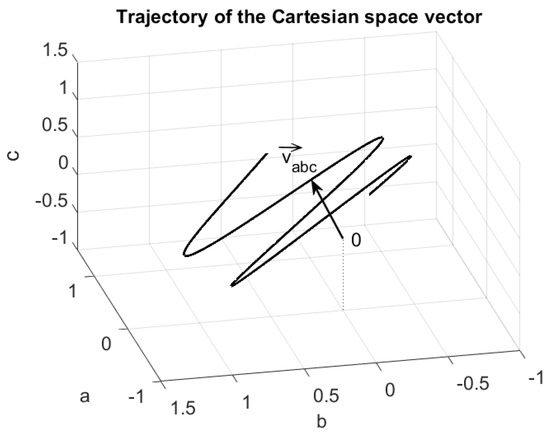
Figure 1.
Example of trajectory of the Cartesian space vector in the orthogonal abc space. If no specific assumptions are made, the trajectory is not within a plane.
The analysis of three-phase quantities in the time domain is often performed by resorting to the Clarke transformation, defined as [10]:
where the transformation matrix is given in its power-invariant form, i.e., . Notice that, from the inverse of Equation (2), we obtain:
where
is an orthonormal basis, i.e.,
In the special case where the zero component in Equation (2) is null, the set of three-phase voltages is such that , i.e., the trajectory of the Cartesian space vector lies on the plane with equation and is defined by the unit vectors (see Figure 2). Therefore, in this case, the three-phase voltages can be completely represented by the two voltages , i.e., by the voltage space vector, defined as:
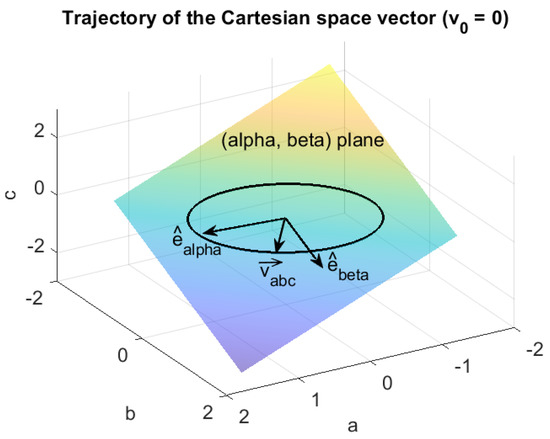
Figure 2.
Example of trajectory of the Cartesian space vector in the orthogonal abc space in case of sinusoidal and null zero component (i.e., ). In this case, the trajectory is lying on the plane with equation and is defined by the unit vectors .
In the general case, i.e., when , the Cartesian space vector does not lie on the plane since the component is also present in Equation (3). In fact, it can be easily shown from Equation (3) that the general equations to recover the phase variables from the space vector Equation (6) and the zero component can be written:
where . Thus, the locus of the zero component is the line along the direction perpendicular to the plane , moving the trajectory of the Cartesian space vector outside the plane . Notice that this property holds regardless of the time behavior of the variables, i.e., under steady-state or transient conditions.
2.1. Balanced and Unbalanced Sinusoidal Steady State
Let us consider a set of sinusoidal three-phase voltages with angular frequency and a zero component (i.e., the balanced case). In this case, the trajectory of the Cartesian space vector lies on the plane (Figure 2), and the corresponding space vector Equation (6) is given by:
where, according to the well-known Symmetrical Component Transformation (SCT) operating on the phasors , and are the phasors of the positive and negative (complex conjugate)-sequence components given by [1]:
where the transformation matrix S is in its power-invariant form, i.e., .
The trajectory of the space vector in Equation (8) is elliptical (Figure 2), with semi-major and semi-minor axes given by [22]:
and the inclination angle by:
As a special case, when the negative-sequence component , the trajectory of the space vector becomes circular with a radius .
In the more general case, where the set of sinusoidal three-phase voltages , with angular frequency , has a zero component (i.e., the unbalanced case), the trajectory of the Cartesian space vector is still planar, but the plane is different from the plane. Thus, the effect of a sinusoidal steady-state zero component is the definition of a new plane where the trajectory of lies. This point can be proven by observing that, since each phase voltage (i.e., , , or ) is a sine wave with angular frequency , such voltage can be seen as a solution of a simple harmonic oscillator defined by a homogeneous second-order differential equation. Since this is true for each phase voltage, the second-order differential equation can be written for the Cartesian space vector [20]:
Thus, the solution can be written as a linear combination of two sine waves:
where and are constant vectors given by the initial conditions:
Equation (13) is the vector representation of a plane defined by the vectors , and the axes origin. Therefore, the trajectory of the Cartesian space vector is always planar and lying on the plane . Such a plane becomes the plane in the special case of the null zero component (i.e., ), whereas the difference with the plane increases as the zero component increases, i.e., for increasing unbalance (see Figure 3). Notice that, in Figure 3, the vectors terminate on the ellipse because of Equation (14), whereas the unit vectors define the plane and, in general, they do not terminate on the ellipse on the plane.
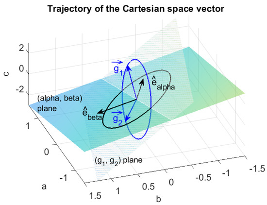
Figure 3.
Trajectory of the Cartesian space vector in the orthogonal abc space in the case of sinusoidal waves . The black line ellipse refers to the case of the null zero component (see Figure 2), whereas the blue line ellipse refers to the case . The zero component results in an elliptical trajectory lying on the plane defined by the vectors instead of the plane.
2.2. Transient Conditions
The dynamics of a three-phase network can be analyzed through the Clarke transformation Equation (2) and the use of voltage/current space vectors defined as in Equation (6). In fact, under the assumption of a symmetrically configured three-phase network, it is well-known that the original network can be studied as two uncoupled networks [21]:
- The space vector network, where all the voltages and currents are defined as space vectors, and the three-phase components are diagonalized by the Clarke transformation (e.g., a three-phase symmetrical mutual inductor with phase self-inductances and mutual inductances , corresponds to the inductance in the space-vector domain after diagonalization through the Clarke transformation);
- The zero-component network, where all the circuit variables are the zero-component variables, the three-phase components are given by Clarke diagonalization (e.g., in the example mentioned above), and single-phase networks (e.g., the fourth wire) connected to the three-phase network are taken into account.
Once the two uncoupled equivalent circuits (i.e., the space-vector and the zero-component circuits) are defined, the conventional state-space equations can be written and solved. Therefore, for the space-vector circuit, we can write the dynamic model [21]:
where is the vector of the space-vector state variables, and is the vector of the space-vector inputs. The matrices A and B are given by the conventional matrices of the state-space approach.
The solution for each state variable (i.e., the generic component of the vector ) can be written as:
where, for the sake of simplicity, the case of N distinct eigenvalues was considered, and the complex coefficients can be determined by setting the initial conditions. Notice that the steady-state component of the solution Equation (16) has the form of Equation (8), whereas the transient component decreases to zero for a stable network.
As far as the zero components are considered, the solution of the corresponding state-space model for the generic state variable can be written in the following form:
where the eigenvalues are different from the eigenvalues in Equation (16) since the zero-component circuit has different topology/parameters.
According to the properties previously derived, the space-vector solution Equation (16) lies on the plane, whereas the zero-component solution Equation (17) (if present) provides a component orthogonal to the plane, leading to a non-planar total solution for the corresponding Cartesian space vector. In general terms, by assuming a transient starting at , the total transient solution Equations (16) and (17) describe the trajectory of the corresponding Cartesian space vector from the steady-state plane for towards a new steady-state plane for , where the steady-state plane can be the plane in the special case of the null zero component.
2.3. The Park Transformation
Let us consider an orthogonal reference frame dq (i.e., direct and quadrature axes) rotating at angular speed on the plane. The components of the Cartesian space vector on the rotating axes dq can be readily obtained by rotating the components by the angle . Thus, the Park transformation can be seen as a composite transformation, where the Clarke transformation is followed by axes rotation [18]:
Notice that, in Equation (18), the zero component remains unchanged. Moreover, for , the dq components equal the components.
The space vector defined on the rotating frame dq is given by:
According to Equation (18), the relationship between the space-vector Equation (6), defined on the fixed axes , and the space-vector Equation (19), defined on the rotating axes dq, can be written:
Using Equation (20) in Equation (16) (i.e., multiplying Equation (16) by ) allows us to highlight the following important properties of transient space-vector solutions when the Park transformation is used:
- The positive-sequence component of the steady-state solution becomes the constant phasor . Thus, the dq components and are constant values.
- The negative-sequence component of the steady-state solution becomes the space vector rotating at double negative speed. Corresponding dq components are second-harmonic sine waves.
- Transient components have a negative frequency shift equal to . In particular:
- For real eigenvalues : each term becomes , thus we obtain a damped space vector rotating at negative speed , and the corresponding dq components are damped sine waves at .
- For a couple of complex conjugate eigenvalues : we obtain the terms and , corresponding to damped space vectors rotating at the shifted angular speeds and . The related dq components contain damped sine waves with shifted angular frequencies and .
3. Test Cases and Discussion
The theoretical properties and results derived in Section 2 are validated and highlighted in this section by resorting to three significant case studies. The first case study consists in a three-phase network leading to a first-order circuit in the space-vector domain, whereas the second case study leads to a second-order circuit in the space-vector domain. In both the cases, the fourth wire is also involved in the transients. The third case study is a three-bus power system. The proposed networks are solved analytically by resorting to the general approach based on the Clarke transformation and the space vectors. The analytical results, however, have been properly checked through numerical simulations with Matlab/Simulink.
3.1. First Case Study: First-Order Circuit in the Space-Vector Domain
Figure 4a shows a three-phase network including a three-phase mutual inductor and resistive elements. The three-phase resistor and the grounding resistor are both inserted at by closing the corresponding switches. The equivalent circuits in the space-vector domain and in the zero-component domain are shown in Figure 4b,c, respectively. In particular, notice that, for the space vectors, the inductance , whereas for the zero components, . Moreover, it is well-known that the single-phase ground network has no effect on the space-vector equivalent circuit since each three-phase wye connection is equivalent to a short circuit for space vectors. On the contrary, in the zero-component equivalent circuit, the single-phase ground network holds its topology, but resistive parameters must be multiplied by the factor 3 (i.e., ).
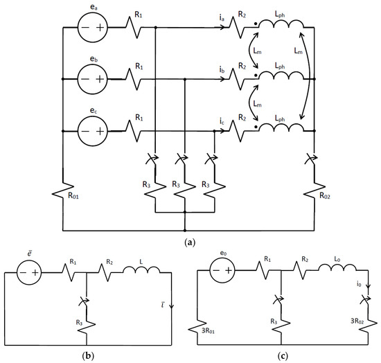
Figure 4.
Three-phase network (a) leading to a first-order circuit in both the space-vector domain (b) and the zero-component domain (c).
The space-vector equivalent circuit in Figure 4b is a first order circuit whose analytical solution for the inductor current can be written in the usual form:
where is the initial condition, , and is the steady-state solution given by:
where , //, and:
The initial condition in Equation (21) can be readily calculated by evaluating the steady-state solution at before the operation of the switch (i.e., by considering the switch as an open circuit):
The zero-component equivalent circuit in Figure 4c is a conventional first-order circuit whose analytical solution can be written as:
where is the initial condition ( in this specific case), , and is the steady-state solution corresponding to the phasor solution:
where , and .
Once the space vector and the zero component are calculated, the phase variables abc can be recovered through Equation (7) when written in terms of currents. Therefore, the Cartesian space vector , the and components of the space vector , and the Park space vector with the corresponding d and q components can be readily calculated from the relevant relationships reported in Section 2.
A total of two different source conditions were considered for the three-phase network in Figure 4. First, a three-phase voltage source with a negative-sequence component . Second, a three-phase voltage source with . In both cases, the zero component of the three-phase voltage source was different from zero. This choice was made to put into evidence the effects of source unbalancing and the source zero component. The circuit parameters were selected as follows: . Notice that the numerical values of the circuit parameters were not related to a specific application, but they were selected with the only objective of putting clearly into evidence the properties of the circuit under analysis.
3.1.1. Three-Phase Voltage Source with
Figure 5 shows the trajectory of the Cartesian space vector . The black line corresponds to the previous steady state (i.e., the steady-state condition for ). At , the curve (in red color) leaves the black trajectory and shows a transient trajectory towards the new steady state. Notice that, for , the trajectory lies on the plane because the zero component (in fact, all the switches were open for ). On the contrary, since the new steady-state condition has (due to the connection of ), the corresponding steady-state trajectory lies on the plane defined by Equation (14) when written for .
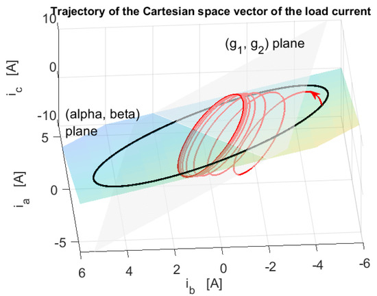
Figure 5.
Trajectory of the Cartesian space vector in the case . The black line shows the steady-state trajectory for , whereas the red line shows the transient behavior, starting at , converging towards the new steady state. The black steady-state curve lies on the plane because for , whereas the new steady-state trajectory lies on the new plane .
Figure 6a shows the trajectory of the space vector on the plane. The steady-state trajectory at the end of the transient is circular since, in this case, the negative-sequence component of the current is zero (as a consequence of the assumption ). The corresponding time-domain behavior of the real and the imaginary parts of the space vector , i.e., the components and , is shown in Figure 6b.
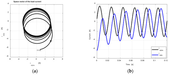
Figure 6.
Trajectory of the space vector on the plane (a) and time-domain behavior of the corresponding and components (b) in the case . In this case, the space-vector trajectory of the new steady state is circular.
Figure 7 shows the behavior of the zero-component current , which is responsible for driving the Cartesian space vector in Figure 5 from the plane to the plane.
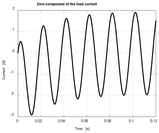
Figure 7.
Transient behavior of the zero-component current responsible for driving the Cartesian space vector in Figure 5 from the plane to the plane.
Figure 8a shows the trajectory of the Park space vector on the dq plane. The trajectory converges towards the positive-sequence phasor (blue line) corresponding to the new steady-state solution. Figure 8b shows the corresponding time-domain behavior of the d and q components of the Park space vector , i.e., the currents and , converging towards the real part and the imaginary part of the positive-sequence phasor in Figure 8a (blue line).
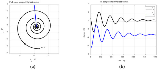
Figure 8.
Trajectory of the Park space vector on the plane (a) and time-domain behavior of the corresponding and components (b) in the case . The straight blue line in (a) shows the steady-state phasor at the end of the transient, i.e., the positive-sequence phasor.
3.1.2. Three-Phase Voltage Source with
Figure 9 shows the trajectory of the Cartesian space vector . Also in this case, as in Figure 5, for , the trajectory lies on the plane because the zero component , and since the new steady-state condition has , the corresponding steady-state trajectory lies on the plane defined by Equation (14) when written for .
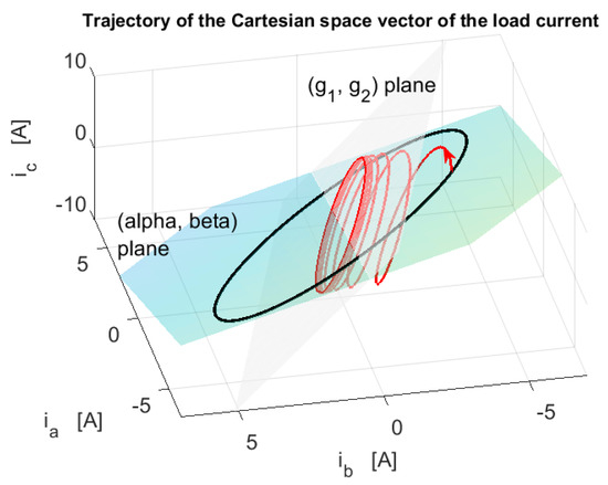
Figure 9.
Trajectory of the Cartesian space vector in the case . The black line shows the steady-state trajectory for , whereas the red line shows the transient behavior, starting at , converging towards the new steady state. The black steady-state curve lies on the plane because for , whereas the new steady-state trajectory lies on the new plane .
Figure 10a shows the trajectory of the space vector on the plane. In this case, the steady-state trajectory at the end of the transient is elliptical since the negative-sequence component of the current is different from zero (as a consequence of the assumption ). The corresponding time-domain behavior of the real and the imaginary parts of the space vector , i.e., the components and , is shown in Figure 10b.
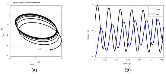
Figure 10.
Trajectory of the space vector on the plane (a) and time-domain behavior of the corresponding and components (b) in the case . In this case, the space-vector trajectory of the new steady state is elliptical.
Notice that the zero-component current is not affected by the negative-sequence component in the voltage source; therefore, its time-domain behavior is still the behavior represented in Figure 7.
Figure 11a shows the trajectory of the Park space vector on the dq plane. The straight blue line shows the positive-sequence phasor. In this case, however, the new steady-state trajectory is a circular trajectory (centered on the positive-sequence phasor) corresponding to the negative-sequence phasor rotating at double (negative) angular frequency . This is apparent in Figure 11b where, according to the theory presented in Section 2, both a transient and a steady-state component can be distinguished.
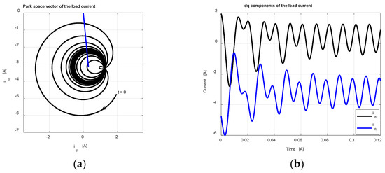
Figure 11.
Trajectory of the Park space vector on the plane (a) and time-domain behavior of the corresponding and components (b) in the case . The straight blue line in (a) shows the positive-sequence phasor of the steady-state solution. In this case, the new steady-state trajectory is a circular trajectory (centered on the positive-sequence phasor) corresponding to the negative-sequence phasor rotating at double (negative) angular frequency . This is apparent in (b) where, according to the theory, both a transient and a steady-state component at can be distinguished.
3.2. Second Case Study: Second-Order Circuit in the Space-Vector Domain
Figure 12a shows a three-phase network including a three-phase mutual inductor, a three-phase capacitor, and resistive elements. The three-phase capacitor and the ground resistor are inserted at by closing the switch. The equivalent circuits in the space-vector domain and in the zero-component domain are shown in Figure 12b,c, respectively. In particular, notice that, for the space vectors, the inductance , whereas for the zero components, . Moreover, the single-phase ground network has no effect on the space-vector equivalent circuit since each three-phase wye connection is equivalent to a short circuit for space vectors. On the contrary, in the zero-component equivalent circuit, the ground resistance must be multiplied by the factor 3, whereas the wye connection of the mutual inductor corresponds to an open circuit.
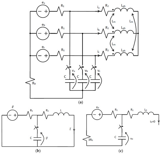
Figure 12.
Three-phase network (a) leading to a second-order circuit in the space-vector domain (b) and a first-order circuit in the zero-component domain (c).
The space-vector equivalent circuit in Figure 12b is a second-order circuit whose conventional state-space representation, according to Equation (15), is given by [21]:
The analytical solution for the inductor current and the capacitor voltage can be written in the usual form:
where are the eigenvalues of the state matrix A (here, distinct eigenvalues are assumed), and are the steady-state solutions, and are the constant coefficients depending on the initial state:
where .
The initial condition in (30) can be readily calculated by evaluating the steady-state solution at before the operation of the switch (i.e., by considering the switch as an open circuit):
whereas the initial condition is a given data. For the sake of simplicity, hereafter, we assume .
The zero-component equivalent circuit in Figure 12c is a conventional first-order RC circuit (in fact ) whose analytical solution can be written as:
where is the initial condition ( in this specific case), , and is the steady-state solution corresponding to the phasor solution:
Once the space vectors , and the zero components , were calculated, the phase variables abc can be recovered through Equation (7) when written in terms of currents and voltages. Therefore, the Cartesian space vectors , , the and space-vector components, and the Park space vectors , with the corresponding d and q components can be readily calculated from the relevant relationships reported in Section 2.
Similar to Section 3.1, two different source conditions were considered for the three-phase network in Figure 12. First, a three-phase voltage source with a negative-sequence component . Second, a three-phase voltage source with . In both cases, the zero component of the three-phase voltage source was different from zero. This choice was made to put into evidence the effects of source unbalancing and the source zero component.
The circuit parameters were selected as follows: , . Notice that the numerical values of the circuit parameters were not related to a specific application, but they were selected with the only objective of putting clearly into evidence the properties of the circuit under analysis. In particular, the selected parameters lead to complex conjugate eigenvalues . Thus, since the imaginary part 316 is very close to the source angular frequency (where ), according to Equation (2), the Park space vectors contain a damped component with a frequency close to zero and a damped component with nearly double frequency . This point is clarified by the results reported in the following sections.
3.2.1. Three-Phase Voltage Source with
Figure 13 shows the trajectory of the Cartesian space vector . The black line corresponds to the previous steady state (i.e., the steady-state condition for ). At , the curve (in red color) leaves the black trajectory and shows a transient trajectory towards the new steady state. Notice that the transient trajectory also lies on the plane because the zero component (in fact, the wye connection of the mutual inductor is not connected to the single-phase network).
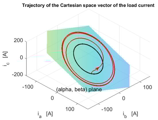
Figure 13.
Trajectory of the Cartesian space vector in the case . The black line shows the steady-state trajectory for , whereas the red line shows the transient behavior, starting at , converging towards the new steady state. Both the black steady-state trajectory and the transient trajectory lie on the plane because .
Figure 14a shows the trajectory of the space vector on the plane. The steady-state trajectory at the end of the transient is circular since, in this case, the negative-sequence component of the current is zero (as a consequence of the assumption ). The corresponding time-domain behavior of the real and the imaginary parts of the space vector , i.e., the components and , is shown in Figure 14b.
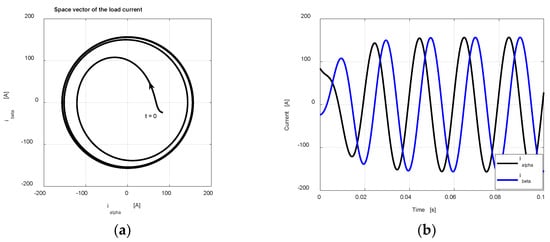
Figure 14.
Trajectory of the space vector on the plane (a) and time-domain behavior of the corresponding and components (b) in the case . In this case, the space-vector trajectory of the new steady state is circular.
Figure 15a shows the trajectory of the Park space vector on the dq plane. The trajectory converges towards the positive-sequence phasor (blue line) corresponding to the new steady-state solution. Figure 15b shows the corresponding time-domain behavior of the d and q components of the Park space vector , i.e., the currents and , converging towards the real part and the imaginary part of the positive-sequence phasor in Figure 15a (blue line). As mentioned before, due to the specific numerical values of the imaginary part of the eigenvalues, we expect transient components at . This is apparent in Figure 15b, where an oscillating behavior with a period (i.e., half period with respect to the source frequency ) is put into evidence.
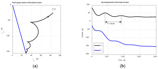
Figure 15.
Trajectory of the Park space vector on the plane (a) and time-domain behavior of the corresponding and components (b) in the case . The straight blue line in (a) shows the steady-state phasor at the end of the transient, i.e., the positive-sequence phasor.
Figure 16 shows the trajectory of the Cartesian space vector . Since the assumed initial condition is , the transient trajectory starts at the axes’ origin. Moreover, due to the zero component in the voltage source, the capacitor voltages have a transient behavior including the zero component This component is responsible for a transient trajectory converging to a plane different from the plane.
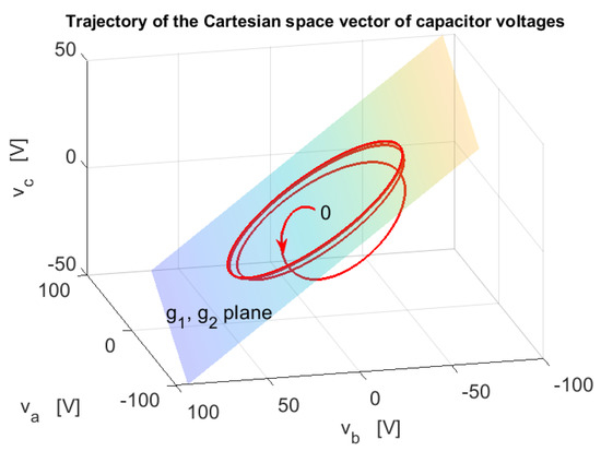
Figure 16.
Trajectory of the Cartesian space vector in the case . The red line shows the transient behavior, starting at , converging towards the new steady state on the plane.
Figure 17a shows the trajectory of the space vector on the plane. The steady-state trajectory at the end of the transient is circular since, in this case, the negative-sequence component of the voltage is zero (as a consequence of the assumption ). The corresponding time-domain behavior of the real and the imaginary parts of the space vector , i.e., the components and , is shown in Figure 17b.
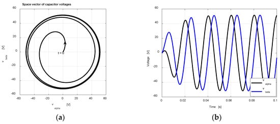
Figure 17.
Trajectory of the space vector on the plane (a) and time-domain behavior of the corresponding and components (b) in the case . In this case, the space-vector trajectory of the new steady state is circular.
Figure 18 shows the behavior of the zero-component voltage , which is responsible for driving the Cartesian space vector in Figure 16 from the axes’ origin to the plane instead of the plane.
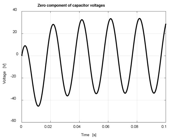
Figure 18.
Transient behavior of the zero-component voltage responsible for driving the Cartesian space vector in Figure 16 from the axes’ origin to the plane instead of the plane.
Figure 19a shows the trajectory of the Park space vector on the dq plane. The trajectory converges towards the positive-sequence phasor (blue line) corresponding to the new steady-state solution. Figure 19b shows the corresponding time-domain behavior of the d and q components of the Park space vector , i.e., the voltages and , converging towards the real part and the imaginary part of the positive-sequence phasor in Figure 19a (blue line). Also in this case, due to the specific numerical values of the imaginary part of the eigenvalues, we expect transient components at . This is apparent in Figure 19b, where an oscillating behavior with a period (i.e., half period with respect to the source frequency ) is put into evidence.
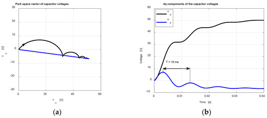
Figure 19.
Trajectory of the Park space vector on the plane (a) and time-domain behavior of the corresponding and components (b) in the case . The straight blue line in (a) shows the steady-state phasor at the end of the transient, i.e., the positive-sequence phasor.
3.2.2. Three-Phase Voltage Source with
Figure 20 shows the trajectory of the Cartesian space vector . The black line corresponds to the previous steady state (i.e., the steady-state condition for ). At , the curve (in red color) leaves the black trajectory and shows a transient trajectory towards the new steady state. Notice that the transient trajectory also lies on the plane because the zero component (in fact, the wye connection of the mutual inductor is not connected to the single-phase network).
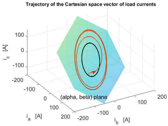
Figure 20.
Trajectory of the Cartesian space vector in the case . The black line shows the steady-state trajectory for , whereas the red line shows the transient behavior, starting at , converging towards the new steady state. Both the black steady-state trajectory and the transient trajectory lie on the plane because .
Figure 21a shows the trajectory of the space vector on the plane. The steady-state trajectory at the end of the transient is elliptical since, in this case, the negative-sequence component of the current is not zero (as a consequence of the assumption ). The corresponding time-domain behavior of the real and the imaginary parts of the space vector , i.e., the components and , is shown in Figure 21b.
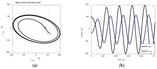
Figure 21.
Trajectory of the space vector on the plane (a) and time-domain behavior of the corresponding and components (b) in the case . In this case, the space-vector trajectory of the new steady state is elliptical.
Figure 22a shows the trajectory of the Park space vector on the dq plane. The trajectory converges towards a circle centered on the positive-sequence phasor (blue line). The circular steady-state trajectory is due to the negative-sequence component of the solution. Figure 22b shows the corresponding time-domain behavior of the d and q components of the Park space vector , i.e., the currents and , converging towards the real part and the imaginary part of the positive-sequence phasor in Figure 22a (blue line), with a superimposed double-frequency solution due to the negative-sequence component. As mentioned before, due to the specific numerical values of the imaginary part of the eigenvalues, we expect transient components at . This is apparent in Figure 22b, where such a transient oscillating component with a period (i.e., half period with respect to the source frequency ) is superimposed on the double-frequency steady-state solution due to the negative-sequence component.
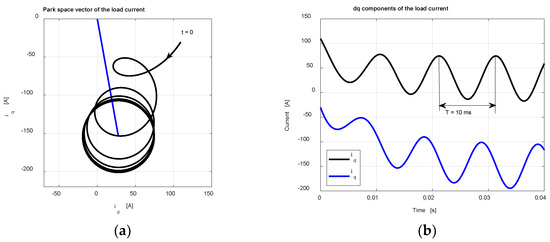
Figure 22.
Trajectory of the Park space vector on the plane (a) and time-domain behavior of the corresponding and components (b) in the case . The straight blue line in (a) shows the positive-sequence phasor where the steady-state circular trajectory is centered.
Figure 23 shows the trajectory of the Cartesian space vector . Since the assumed initial condition is , the transient trajectory starts at the axes’ origin. Moreover, due to the zero component in the voltage source, the capacitor voltages have a transient behavior including the zero component This component is responsible for a transient trajectory converging to a plane different from the plane.
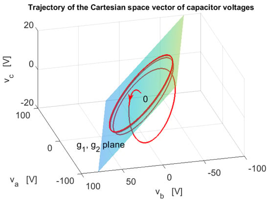
Figure 23.
Trajectory of the Cartesian space vector in the case . The red line shows the transient behavior, starting at , converging towards the new steady state on the plane.
Figure 24a shows the trajectory of the space vector on the plane. The steady-state trajectory at the end of the transient is elliptical since, in this case, the negative-sequence component of the voltage is not zero (as a consequence of the assumption ). The corresponding time-domain behavior of the real and the imaginary parts of the space vector , i.e., the components and , is shown in Figure 24b.
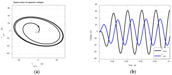
Figure 24.
Trajectory of the space vector on the plane (a) and time-domain behavior of the corresponding and components (b) in the case . In this case, the space-vector trajectory of the new steady state is elliptical.
The zero-component voltage , which is responsible for driving the Cartesian space vector in Figure 23 from the axes’ origin to the plane instead of the plane, is not affected by the negative-sequence component in the voltage source. Therefore, its time behavior is the same as in Figure 18.
Figure 25a shows the trajectory of the Park space vector on the dq plane. The trajectory converges towards a circular trajectory, due to the negative-sequence component, centered on the positive-sequence phasor (blue line). Figure 25b shows the corresponding time-domain behavior of the d and q components of the Park space vector , i.e., the voltages and , converging towards the real part and the imaginary part of the positive-sequence phasor in Figure 25a (blue line), with a superimposed double-frequency steady-state solution due to the negative-sequence component. Also in this case, due to the specific numerical values of the imaginary part of the eigenvalues, we expect transient components at . This is apparent in Figure 25b, where both the transient oscillating behavior and the steady-state oscillating behavior with a period (i.e., half period with respect to the source frequency ) can be identified.
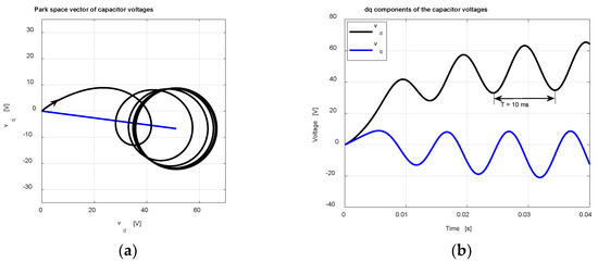
Figure 25.
Trajectory of the Park space vector on the plane (a) and time-domain behavior of the corresponding and components (b) in the case . The straight blue line in (a) shows the positive-sequence phasor where the steady-state circular trajectory is centered.
3.3. Third Case Study: Three-Bus Power System
Figure 26 shows a three-bus medium-voltage (MV) 60 Hz power system [23]. The analytical methods outlined in Section 2 can be used to study the transient behavior of the power system once it is energized by the generator at . Also in this case, the analytical results have been checked against numerical results obtained by means of Matlab/Simulink simulations.
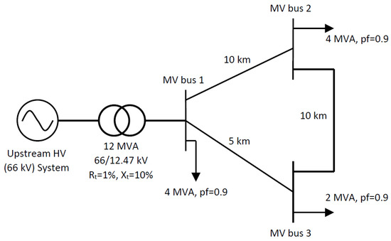
Figure 26.
Three-bus MV power system. Loads are given in terms of apparent power and lagging power factor (pf).
Generator and loads data are reported in Figure 26. The positive-sequence and the zero-sequence impedances of the lines are and , respectively. Notice that, in order to use the analytical results derived in Section 2, the loads must be converted into equivalent impedances. This can be easily done by recalling that the complex power and the impedance of a given load are related by , where is the reference phase-to-phase voltage (i.e., in this case), and the asterisk denotes a complex conjugate. Figure 27 shows the topology of the space-vector equivalent circuit. Notice that the same topology holds for the zero components in case the ground is involved in the current path.
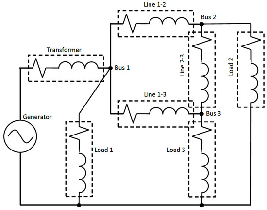
Figure 27.
Topology of the space-vector equivalent circuit of the three-bus power system reported in Figure 26.
The space-vector equivalent circuit corresponding to Figure 27 can be solved by resorting to the conventional state-space approach, leading to the dynamical model in Equation (15). Notice that the effective dynamical order of the circuit in Figure 27 is four (instead of seven) because the seven inductive currents have three independent constraints given by the Kirchhoff Laws at the three buses. By assuming that the network is energized by the generator at , and by setting the generator with a 5% negative-sequence voltage component, the trajectory of the Cartesian space vector of the generator currents is represented in Figure 28. Notice that, since the generator currents have a null zero component, the Cartesian space vector lies on the plane. The space vector of the generator currents is represented in Figure 29a, whereas the corresponding and components are represented in Figure 29b as functions of time. Notice that the steady-state trajectory in Figure 29a is elliptical because of the 5% negative-sequence component in the generator voltage. Figure 30a shows the trajectory of the Park space vector of the generator currents, whereas Figure 30b shows the time-domain behavior of the corresponding dq components. Notice that, in Figure 30a, the negative-sequence component in the steady-state currents results in the small circle around the phasor (blue line) corresponding to the positive-sequence component solution. The negative-sequence component can also be observed in Figure 30b, where oscillations at frequency can be detected. Notice that, in this case, the oscillations have only the component at frequency , whereas the phenomenon of frequency shifting cannot be observed because the eigenvalues of the network in Figure 27 are real eigenvalues (complex conjugate eigenvalues would be possible only for an RLC network).
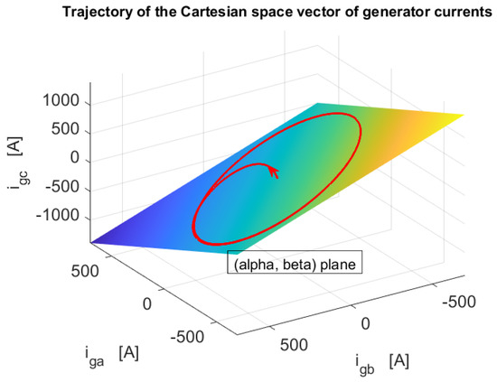
Figure 28.
Trajectory of the Cartesian space vector of the generator currents. The trajectory lies on the plane because the zero component of the currents is null.
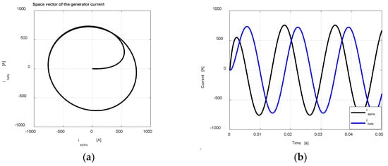
Figure 29.
Space vector of the generator currents on the plane (a) and time-domain behavior of the corresponding and components (b).
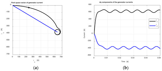
Figure 30.
Park space vector of the generator currents on the plane (a) and time-domain behavior of the corresponding and components (b). The circle in (a) corresponds to the negative-sequence component in the steady-state solution.
Finally, the effect of the zero-component current can be investigated by considering the ground connections of the load and of the secondary of the transformer (normally wye-connected to avoid the circulation of zero-component currents). In this case, the zero-component current has a transient behavior (see Figure 31), leading to a Cartesian space vector lying on the plane (see Figure 32) instead of the plane, as in Figure 28.
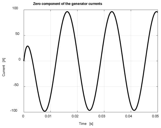
Figure 31.
Time-domain behavior of the zero-component current.
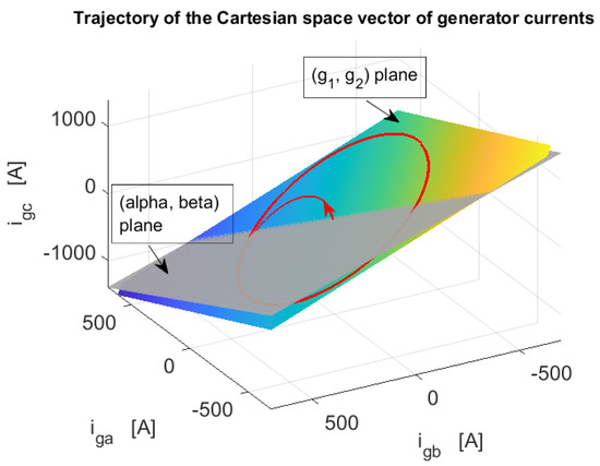
Figure 32.
Trajectory of the Cartesian space vector of the generator currents. The trajectory lies on the plane instead of the plane because of the zero component of the generator currents.
4. Conclusions
The analytical tools used in the paper allow a comprehensive investigation of the properties of three-phase transients with unbalanced sources and involving the fourth wire. In particular, a complete geometrical representation is given by the Cartesian space vector of a three-phase variable, whereas the space vectors based on the Clarke transformation allow us to study the original three-phase transient as a superposition of two independent transients. The dq0 representation provided by the Park transformation was also discussed, and the effects of the frequency shift with respect to the Clarke transformation were shown through specific case studies.
The methodology and the properties derived and discussed in the paper provide a general theoretical framework for three-phase transient analysis. Thus, the paper is intended to provide a theoretical contribution, whereas the selection of numerical methods for the effective solution of time-domain equations is the topic of the cited relevant literature.
Funding
This research received no external funding.
Conflicts of Interest
The author declares no conflict of interest.
References
- Bellan, D.; Pignari, S.A.; Superti-Furga, G. Consistent circuit technique for zero-sequence currents evaluation in interconnected single/three-phase power networks. J. Electr. Syst. 2016, 12, 230–238. [Google Scholar]
- Fortescue, C.L. Method of symmetrical coordinates applied to the solution of polyphase networks. Trans. AIEE 1918, 37, 1027–1140. [Google Scholar]
- Bellan, D. Circuit modeling and statistical analysis of differential-to-common-mode noise conversion due to filter unbalancing in three-phase motor drive systems. Electronics 2020, 9, 1612. [Google Scholar] [CrossRef]
- Das, J.C. Understanding Symmetrical Components for Power System Modeling; Wiley: Hoboken, NJ, USA, 2017. [Google Scholar]
- Chicco, G.; Mazza, A. 100 Years of Symmetrical Components. Energies 2019, 12, 450. [Google Scholar] [CrossRef]
- Bollen, M.H.J.; Yu-Hua Gu, I. On the analysis of voltage and current transients in three-phase power systems. IEEE Trans. Power Deliv. 2007, 22, 1194–1201. [Google Scholar] [CrossRef]
- Mahseredjian, J.; Dinavahi, V.; Martinez, J.A. Simulation tools for electromagnetic transients in power systems: Overview and challenges. IEEE Trans. Power Deliv. 2009, 24, 1657–1669. [Google Scholar] [CrossRef]
- Van der Sluis, L. Transients in Power Systems; John Wiley & Sons Ltd: Chichester, UK, 2001. [Google Scholar]
- Greenwood, A. Electrical Transients in Power Systems, 2nd ed.; Wiley India (P.) Ltd.: New Delhi, India, 1991. [Google Scholar]
- Bellan, D. Clarke transformation solution of asymmetrical transients in three-phase circuits. Energies 2020, 13, 5231. [Google Scholar] [CrossRef]
- Ilic, M.; Zaborszky, J. Dynamics and Control of Large Electric Power Systems; Wiley-IEEE Press: New York, NY, USA, 2000. [Google Scholar]
- Baimel, D.; Belikov, J.; Guerrero, J.M.; Levron, Y. Dynamic Modeling of Networks, Microgrids, and Renewable Sources in the dq0 Reference Frame: A Survey. IEEE Access 2017, 5, 21323–21335. [Google Scholar] [CrossRef]
- Vega-Herrera, J.; Rahmann, C.; Valencia, F.; Strunz, K. Analysis and Application of Quasi-Static and Dynamic Phasor Calculus for Stability Assessment of Integrated Power Electric and Electronic Systems. IEEE Trans. Power Syst. 2021, 36, 1750–1760. [Google Scholar] [CrossRef]
- Stankovic, A.M.; Lesieutre, B.C.; Aydin, T. Modeling and analysis of single-phase induction machines with dynamic phasors. IEEE Trans. Power Syst. 1999, 14, 9–14. [Google Scholar] [CrossRef]
- Miao, Z.; Piyasinghe, L.; Khazaei, J.; Fan, L. Dynamic Phasor-Based Modeling of Unbalanced Radial Distribution Systems. IEEE Trans. Power Syst. 2015, 30, 3102–3109. [Google Scholar] [CrossRef]
- Levron, Y.; Belikov, J. Modeling power networks using dynamic phasors in the dq0 reference frame. Electr. Power Syst. Res. 2017, 144, 233–242. [Google Scholar] [CrossRef]
- Hassani, R.; Mahseradjian, J.; Tshibungu, T.; Karaagac, U. Evaluation of time-domain and phasor-domain methods for power system transients. Electr. Power Syst. Res. 2022, 212, 108335. [Google Scholar] [CrossRef]
- O’Rourke, C.J.; Qasim, M.M.; Overlin, M.R.; Kirtley, J.L., Jr. A geometric interpretation of reference frames and transformations: dq0, Clarke and Park. IEEE Trans. Energy Convers. 2019, 34, 2070–2083. [Google Scholar] [CrossRef]
- Mohanty, R.; Sahu, N.K.; Pradhan, A.K. Time-Domain Techniques for Line Protection Using Three-Dimensional Cartesian Coordinates. IEEE Trans. Power Deliv. 2022, 37, 3740–3751. [Google Scholar] [CrossRef]
- Casado-Machado, F.; Martinez-Ramos, J.L.; Barragán-Villarejo, M.; Maza-Ortega, J.M.; Rosendo-Macías, J.A. Reduced Reference Frame Transform: Deconstructing Three-Phase Four-Wire Systems. IEEE Access 2020, 8, 143021–143032. [Google Scholar] [CrossRef]
- Bellan, D.; Superti-Furga, G. Space-vector state-equation analysis of three-phase transients. J. Electr. Syst. 2018, 14, 188–198. [Google Scholar]
- Bellan, D. Probability Density Function of Three-Phase Ellipse Parameters for the Characterization of Noisy Voltage Sags. IEEE Access 2020, 8, 185503–185513. [Google Scholar] [CrossRef]
- Paranavithana, P.; Perera, S.; Koch, R.; Emin, Z. Global Voltage Unbalance in MV Networks Due to Line Asymmetries. IEEE Trans. Power Deliv. 2009, 24, 2353–2360. [Google Scholar] [CrossRef]


Publisher’s Note: MDPI stays neutral with regard to jurisdictional claims in published maps and institutional affiliations. |
© 2022 by the author. Licensee MDPI, Basel, Switzerland. This article is an open access article distributed under the terms and conditions of the Creative Commons Attribution (CC BY) license (https://creativecommons.org/licenses/by/4.0/).