Article

Application of Modelling and Simulation in Durability Tests of Vehicles and Their Components

1
Faculty of Transport, Warsaw University of Technology, ul. Koszykowa 75, 00-662 Warsaw, Poland
2
Łukasiewicz Research Network—Automotive Industry Institute PIMOT, ul. Jagiellońska 55, 03-301 Warsaw, Poland
Energies 2022, 15(24), 9398; https://doi.org/10.3390/en15249398
Submission received: 15 October 2022 / Revised: 29 November 2022 / Accepted: 6 December 2022 / Published: 12 December 2022
(This article belongs to the Special Issue Motor Vehicles Energy Management)

Abstract

:
The use of simulation and modelling has been proposed for determining the excitations to be applied in the procedures of laboratory testing of a car’s structural components, without the need to test the complete vehicle. The paper presents the general concept as well as an example of the procedure. It covers determining the spectrum and time-domain realization of a load on a selected node of the vehicle structure under durability tests. The author used both the mathematical and physical model of the tractor-semitrailer unit, where the input was considered as a random process resulting from the road profile. He calculated the transmittance modules and the power spectral densities of the vertical force on the joint between the tractor’s fifth wheel and the kingpin of the semitrailer and the extreme values of the dynamic components of this force. The inverse discrete Fourier transform makes it possible to generate the realization of the said force. It can be used in durability studies. The limitation of the work to the testing of a specific structural node reduces the scope and, in consequence, the cost of the process. The method presented may also be used for various types of vehicle models, including hybrid and electric vehicles.

1. Introduction

The new or modified structures of vehicles and their components are subjected to accelerated tests carried out in real or simulated conditions, corresponding to the anticipated conditions of use [1,2,3,4,5,6,7,8,9,10,11,12,13]. For the granting of certificates of various types (e.g., a safety certificate) to a product, an appropriate series of tests must be carried out to confirm the suitability of the product for service in the target operating conditions [10]. Moreover, the product structure should also be tested for its durability and the prototype should undergo validation tests [1,3,4,5,6,7,10,11,12,13]. The tests carried out in real operating conditions (on roads or testing grounds) are very much time-consuming, expensive, and more dangerous than any others. The simulation tests, where simulation stands are used, greatly accelerate the product testing process and ensure good repeatability of results [6,7]. The manufacturers of vehicle’s structural components (component units, subassemblies, and individual parts) are chiefly interested in the testing of their specific products, rather than disregarding the other parts of the vehicle’s structure, which are considered as lying within the responsibilities of the final vehicle manufacturer [4,12,13]. The author formulates here a proposal to use the simulation and modelling for determining the conditions of testing the structural components (component units, subassemblies, and individual parts) without the need to test the complete vehicle. The general concept of this approach has been presented in a condensed form in the publication [14]. Here, an example of its application will be demonstrated. The formulation of a mathematical model that would represent the vehicle’s motion in typical operating conditions will make it possible to carry out simulation tests in the time and/or frequency domain [2,14,15,16,17,18,19,20,21,22] and thus, to determine the time histories of the loads on selected items. The load vs. time curves thus obtained may be used to test the vehicle’s structural nodes of interest, such as vehicle axles, wheel hubs, tires, springs, and damping suspension components, or vehicle coupling devices (e.g., couplings between the fifth wheel and the kingpin, between the towing hook and the trailer’s drawbar towing hitch, etc.). The anticipated benefit would be a limitation of the work scope to the testing of a specific structural node, which will reduce the scope and, in consequence, the “multidimensionality” and cost of the process. This method may be very useful for the testing of both simple and complicated structures of modern vehicles, e.g., the electrical or hybrid ones.

2. Up-to-Date State and the Essence of the Method Proposed

2.1. Examples of Stands for the Simulation of Operating Loads on Vehicles and Their Structural Nodes

The simulation tests of vehicles, their component units, and subassemblies have been carried out all over the world for several decades [1,3,6,7]. In Poland, the role of a leader has been played for many years by the Automotive Industry Institute PIMOT (currently named as Łukasiewicz Research Network—Automotive Industry Institute PIMOT), in the field of both research methodology [6,7] and practical applications [6,7,10]. In the recent years, even private manufacturers operating in the automotive sector have been building research centres and have been implementing the methodology of durability and validation testing of prototypes [12,13]. With this objective in view, a wide variety of advanced test equipment inclusive of control software, being currently available, is made use of (see e.g., [5,11]).
However, the methods of the most accurate replication of the real-world loads acting on vehicles and their structural nodes are continuously sought for the structures being tested to be verified within the shortest time and at the lowest cost possible.

2.2. Methods of the Carrying out of Bench Simulation Tests of the Operating Loads on Vehicles and Their Structural Nodes

It is worth quoting here the words from the publication, the authors of which were engaged in simulation tests for many years [7]: “Bench tests in which vehicle components, assemblies, and complete vehicles are tested in conditions more or less different from those in use, but are carried out in laboratories. This gives better research possibilities and, at the same time, the possibility of evaluating the vehicle in a relatively short time (…). Generally, bench tests are poor in input signals, and are also artificially shaped. However, they provide much greater possibilities of measuring output signals, both in terms of their number and type; moreover, they have a very important feature: repeatability of tests”. The same authors have remarked that every experimental test can be regarded as a simulation of real events, the only difference being in its accuracy, scope, and purpose for which it is carried out.
The simulation stands are specifically designed for their planned use, taking into account in particular the purpose of the tests and the question whether the object under test is to be a complete vehicle or a vehicle part. So, there are facilities intended for cars taken as a whole (i.e., with complete equipment), vehicles partially disassembled, complete component units (such as e.g., engines, transmissions, drive axles, etc.), as well as selected individual component parts.
The experimental simulation tests (on laboratory stands) are carried out in two variants (see Figure 1 based on description published in [7]):
variant 1 (simulation based on the input signals): The signals that control the vibrators of the test stand are predetermined, e.g., based on measurements of the geometric profile of the road surface to be simulated;
variant 2 (simulation based on the output signals): The machine is controlled by external inputs specially shaped so that the values of specific output parameters obtained on the test stand are in compliance with those previously measured during the corresponding road test (carried out in predefined conditions).
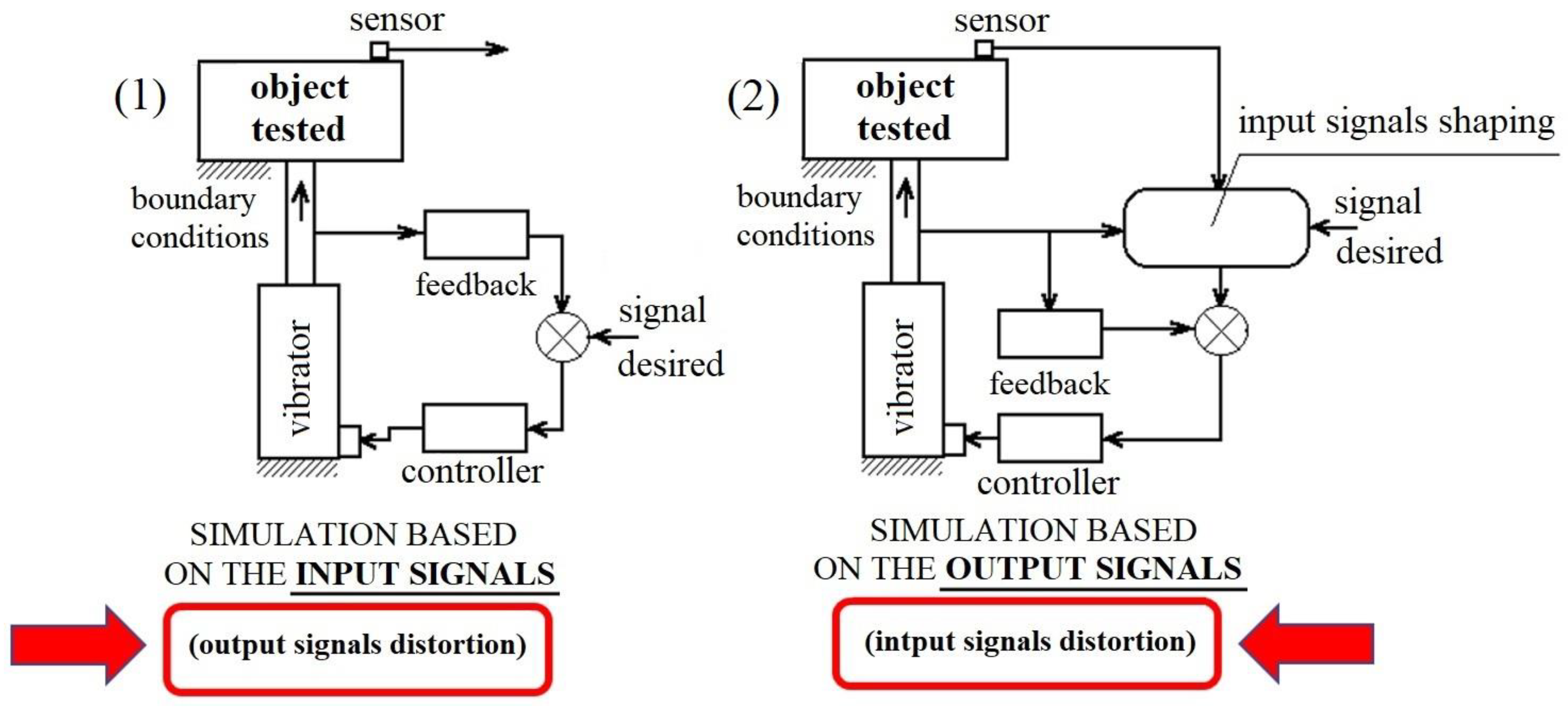
The authors of publication [7] emphasize the fact that in variant 1, there is a risk of distorting the actuators’ output signals if the conditions of the excitation applied to the object under test on the test stand considerably differ from those in reality. The most common example cited is the fact that vehicle’s road wheels do not rotate during bench tests, which significantly affects the dynamic characteristics of the pneumatic tire. On the other hand, it is worth noting that in modern test facilities, the input is applied to a rotating wheel. However, this significantly increases the cost of the stand and of the test itself. For similar reasons, the input signals in variant 2 are intentionally deformed, because the compliance of the selected signal during the bench test with that measured in the corresponding road test conditions is important.
Figure 1. Variants of the approach to the experimental simulation tests. (1)—simulation based on the input signals, (2)—simulation based on the output signals.
Energies 15 09398 g001

2.3. The Essence of the Method Proposed

A digital computer simulation will be carried out, where a mathematical model of the real object, including separate models of inputs and outputs, will be used. The simulation will be built according to variant 1 (based on the input signals), using models of input signals (excitations) that would represent road profile, aerodynamic impact, and internal forces (caused by e.g., driving and braking torques, steering angles applied, etc.) resulting from vehicle driver’s activities.
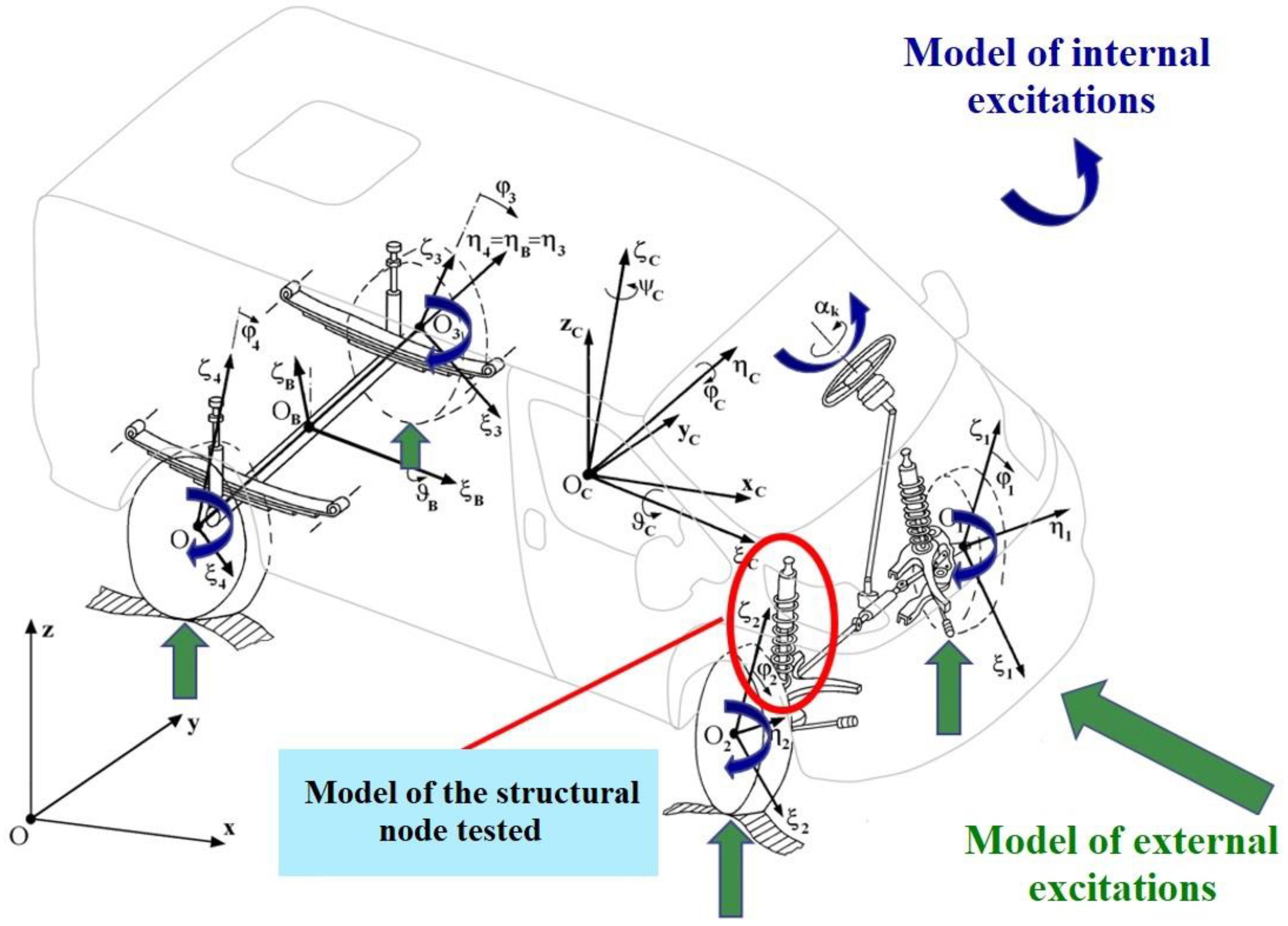
The mathematical model or simulation model of the vehicle contains the model of the structural node of interest together with the model of inputs (excitations) and outputs (Figure 2 and Figure 3). Assuming the excitations that would be representative for the conditions of operation of the object under test, we use the model for determining the excitation acting on the vehicle construction node of interest. The said excitation may be used in the experimental simulation of loads on the structural node on a laboratory test stand, which will reduce the “multidimensionality” and cost of the testing process. This will be very important for the most modern vehicles, e.g., electrical or hybrid designs.
The method as described above may be used to test such vehicle’s structural nodes as vehicle axles, wheel hubs, tires, springs, and damping suspension components, or vehicle coupling devices (e.g., couplings between the fifth wheel and the kingpin, between the towing hook and the trailer’s drawbar towing hitch, etc.).

3. Possible Useful Simulation Models and an Example Procedure of the Method Proposed

3.1. Examples of the Possible Useful Simulation Models of Motion and Dynamics of Road Vehicles

Models of this kind have been used for the last several decades in the research on vehicle motion and dynamics. They have been presented in publications [2,8,15,16,17,22,23,24,25,26]. The author of this paper has built many of his own, original models and simulation programs. He described them in publications [17,18,19]. They can be employed to determine the input signal acting on a selected node of the vehicle structure, as it has been shown schematically in Figure 3 for the case of the spring-damping element of the front wheel suspension of a passenger car.

3.2. Example Procedure Followed When the Modelling and Simulation Is Employed to Determine the Spectrum and Time History of the Load on a Selected Node of the Vehicle Structure Tested for Durability

3.2.1. Structure of the Physical Model of a Tractor-Semitrailer Unit

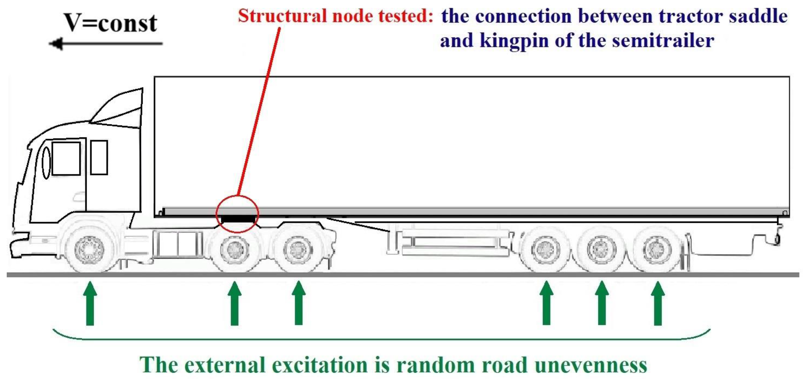
Let us consider the tractor-semitrailer combination in a rectilinear motion with a constant speed V (Figure 4). The structural node examined is the connection between tractor’s fifth wheel and the kingpin of the semitrailer. The excitation is applied as random displacements representing road profile heights.
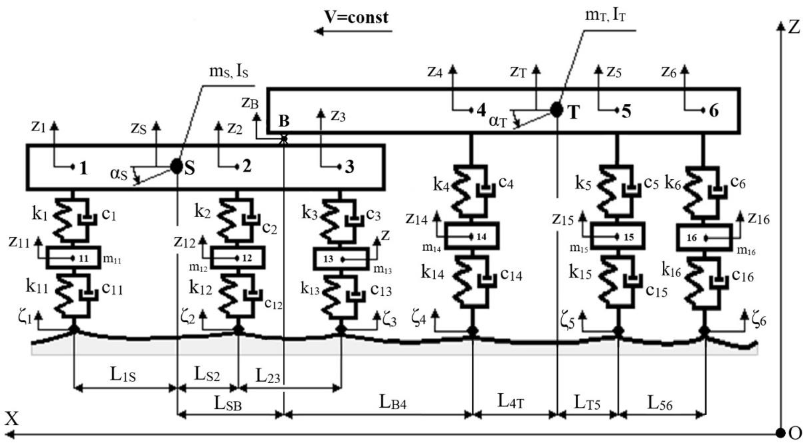
Figure 5 shows a physical model proposed by the author to represent the tractor-semitrailer unit in a rectilinear motion with a constant speed V. It corresponds to the illustration in Figure 4. It should be noted that the structure of this model enables the description of the dynamics of a three-axle truck towing a three-axle trailer with a rigid drawbar connected to the towing vehicle by a ball joint (for flat models: a swivel joint).
The highlighted points of the model are S (centre of mass of the tractor body mass); T (semitrailer body solid’s centre of mass); B (connection between tractor’s fifth wheel and semitrailer’s kingpin); 1, 2, and 3 (points of the tractor body structure located above individual tractor axles); 4, 5, and 6 (points of the body structure of the semitrailer located above individual axles of the semitrailer); 11, 12, and 13 (centres of the unsprung masses of successive tractor axles); 14, 15, and 16 (centres of the unsprung masses of successive axles of the semitrailer). The following coordinates were adopted to describe the movement of the elements of this model: z1, z2, and z3 (vertical displacements of points 1, 2, and 3 of the tractor body, located above the tractor axles); z4, z5, and z6 (vertical displacements of points 4, 5, and 6 of the semitrailer body, the points being located above the semitrailer axles); z11, z12, and z13 (vertical displacements of points 11, 12, and 13, i.e., the tractor axles); z14, z15, and z16 (vertical displacements of points 14, 15, and 16, i.e., the semitrailer axles); zS, zT, and zB (vertical displacements of points S, T, and B); αS (pitch angle of the tractor body solid); and αT (pitch angle of the semitrailer body). All the above displacements (i.e., z1-z6, z11-z16, zS, zT, and zB) and pitch angles (αS and αT) were considered as measured from the state of static equilibrium on a perfectly even, horizontal road surface.
The road profile heights under successive axles of the tractor-semitrailer unit are denoted as ζi, i = 1, …, 6. The movement of the unit as a whole is described in the OXZ coordinate system attached to the road; the vertical movements of the highlighted points (as already mentioned) are specified as relative to the positions of static equilibrium on a perfectly even, horizontal road surface. The symbols mS and mT mean the masses of the truck tractor and semitrailer body solids, respectively. IS and IT are, respectively, the moments of inertia of the tractor and semitrailer body solids with respect to the horizontal transverse axes through points S and T. The values of the unsprung masses associated with successive wheel axles are denoted as mi, where i = 11, 12, …, 16. The stiffness of the suspensions of successive wheel axles is denoted as ki, where i = 1, 2, …, 6. The radial stiffness of the tires of successive wheel axles is denoted as ki, where i = 11, 12, …, 16. The viscous damping coefficients for suspensions are denoted as ci, where i = 1, 2, …, 6. The viscous damping coefficients in the radial direction of the tires of successive wheel axles are denoted as ci, i = 11, 12, …, 16. Figure 5 also shows the horizontal distances Lij between the marked points “i” and “j”.

3.2.2. Main Simplifying Assumptions

  • The speed of the vehicle combination in the analysed rectilinear motion is constant, V = const.
  • The road surface is non-deformable and uneven. The road profile is considered as a Gaussian (normal), stationary, and ergodic random process. It is described as recommended by ISO [27,28]. Its shortest and longest wavelength is 0.1 m and 100 m, respectively. Apart from this unevenness, the road surface is level with no longitudinal slope.
  • The spring and damping suspension elements have linear characteristics.
  • The spring and damping properties of the road wheels are linear in the radial direction.
  • The phenomena of road wheel lift-off and hop and the wheel suspension blocking during compression or rebound are ignored.
  • The described translational and angular displacements are considered in relation to the static equilibrium position, for the horizontal and ideally smooth road surface.
  • The said relative displacements are so small that Simplifications (1) and (2) may be adopted.
    sin αS = αS,  cos αS = 1
    sin αT = αT,  cos αT = 1
  • The longitudinal components of the movement of points 1–6, 11–16, S, T, and B are omitted.
  • The smoothing properties of the tires are considered in the form of a “fixed footprint tire model (FFTM)” [17], leading to the filtration of the power spectral density (PSD) of the road profile heights.
  • If the model of the vehicle combination is interpreted not as a tractor-semitrailer unit but as a car towing a trailer (coupled by a ball hook-drawbar joint or a rotary joint in the case of a two-dimensional model as discussed herein), then the drawbar of the trailer is rigidly connected to the trailer body. There are no articulated joints (in the trailer), as is the case with trailers with at least two axles.

3.2.3. Indication of Generalized Coordinates and Their Relations with the Adopted Coordinates Describing the Movement of the Vehicle Combination under Analysis

The following set of independent coordinates (generalized coordinates) was adopted: z1, z2, zT, z11, z12, z13 z14, z15, and z16. They have been defined in the description of the model in Figure 5. For the aforementioned assumptions, these coordinates do not depend on each other and fully describe the analysed motion of the vehicle combination with a constant speed of V. The model adopted (Figure 5) has, therefore, nine degrees of freedom. For a mathematical model of the system under analysis to be built, it is necessary to define, in the description of its dynamics, the quantities needed (apart from the generalized coordinates) for the calculation of elastic and damping forces (in the wheel suspension and tires), kinetic energy, potential energy, Rayleigh dissipation function, and inertia forces. These are the coordinates zS, z3, z4, z5, z6, αS, αT presented above, related to the generalized coordinates by Equations (3)–(13).
zS = (z1·LS2 + z2·L1S)/L12
αS = (z2 − z1)/L12
αT = (zT − zB)/LBT = zT/LBT − αS·LSB/LBT − zS/LBT
z3 = zS + αS·LS3
z4 = zT − αT·L4T
z5 = zT + αT·LT5
z6 = zT + αT·LT6
where
LBT = LB4 + L4T
L12 = L1S + LS2
LS3 = LS2 + L23
LT6 = LT5 + L56
By analogy to Equations (3)–(9) (plus (10)–(13)), the relations concerning the first and second derivatives (with respect to time) of coordinates zS, z3, z4, z5, z6, αS, αT may be formulated as functions of the first and second derivatives of the generalized coordinates and parameters of the system analysed.

3.2.4. Other Important Relationships to Be Defined before Deriving the Equations of Motion

It is necessary to determine additional quantities that are needed to calculate the kinetic energy, potential energy, and Rayleigh dissipative function. These are suspension deflections ui for the ith axle (i = 1, …, 6), radial deflections uj of the road wheel associated with the jth unsprung mass (j = 11, …, 16), and their first derivatives with respect to time. The first and second groups of the said quantities are described by Equations (14)–(25).
u1 = z11 + αS·L1S − zS
u2 = z12 − αS·LS2 − zS
u3 = z13 − αS·LS3 − zS
u4 = z14 + αT·L4T − zT
u5 = z15 − αT·LT5 − zT
u6 = z16 − αT·LT6 − zT
u11 = ζ1 − z11
u12 = ζ2 − z12
u13 = ζ3 − z13
u14 = ζ4 − z14
u15 = ζ5 − z15
u16 = ζ6 − z16
Attention should be paid to the phase shift θi between the kinematic inputs ζi(t) on the road wheels of successive axles, in relation to the first axle. The inputs are described by Equations (26)–(30). Note: the following symbols have been adopted: V [km/h], v [m/s].
ζ2(t) = ζ1(t − θ2) where θ2 = L12/v
ζ3(t) = ζ1(t − θ3) where θ3 = (L12 + L23)/v
ζ4(t) = ζ1(t − θ4) where θ4 = (L1S + LSB + LB4)/v
ζ5(t) = ζ1(t − θ5) where θ5 = (L1S + LSB + LB4 + L4T + LT5)/v
ζ6(t) = ζ1(t − θ6) where θ6 = (L1S + LSB + LB4 + L4T + LT5 + L56)/v
The relations concerning the first derivatives (with respect to time) of the suspension deflection ui for the ith vehicle axle (i = 1, …, 6) and of the radial deflections uj of the road wheel associated with the jth unsprung mass (j = 11, …, 16) are analogous to Equations (14)–(25) (plus (26)–(30)).

3.2.5. Equations of Motion—Mathematical Model

Lagrange equations of the second kind were used:
D dt ( E k q ˙ i ) E k q i + E p q i + R q ˙ i = Q i i = 1 ,   2 ,   ,   9
The generalized coordinates are:
q1 = z1, q2 = z2, q3 = zT, q4 = z11, q5 = z12, q6 = z13, q7 = z14, q8 = z15, q9 = z16
Kinetic energy of the system:
E k = ½ · ( m S · z ˙ S 2 + I S · α ˙ S 2 + m 11 · z ˙ 11 2 + m 12 · z ˙ 12 2 + m 13 · z ˙ 13 2 +                               + m T · z ˙ T 2 + I T · α ˙ T 2 + m 14 · z ˙ 14 2 + m 15 · z ˙ 15 2 + m 16 · z ˙ 16 2 )
Potential energy of the system:
E p = ½ · ( k 1 · u 1 2 + k 2 · u 2 2 + k 3 · u 3 2 + k 11 · u 11 2 + k 12 · u 12 2 + k 13 · u 13 2 + + k 4 · u 4 2 + k 5 · u 5 2 + k 6 · u 6 2 + k 14 · u 14 2 + k 15 · u 15 2 + k 16 · u 16 2 )
Rayleigh dissipative function:
R = ½ · ( c 1 · u ˙ 1 2 + c 2 · u ˙ 2 2 + c 3 · u ˙ 3 2 + c 11 · u ˙ 11 2 + c 12 · u ˙ 12 2 + c 13 · u ˙ 13 2 + + c 4 · u ˙ 4 2 + c 5 · u ˙ 5 2 + c 6 · u ˙ 6 2 + c 14 · u ˙ 14 2 + c 15 · u ˙ 15 2 + c 16 · u ˙ 16 2 )
Due to the assumptions made:
Qi = 0   i = 1, 2, …, 9
When Equations (32)–(36) were substituted to (31), taking into account (3)–(25) (and analogous relations concerning the first derivatives), the following equations were obtained (after complex transformations), which can be written in the matrix form (37):
M · q ¨ + C · q ˙ + K · q = C ζ · ζ ˙ + K ζ · ζ
Equation (37) uses the matrix symbols (their dimensions are also given here): inertia M9×9, viscous damping C9×9, stiffness K9×9, kinematic excitation impact modified by damping in the pneumatic tire Cζ9×6, and kinematic excitation impact modified by the radial elasticity of the pneumatic tire Kζ9×6. The vectors of coordinates (displacements), velocities, and generalized accelerations are denoted as q , q ˙ , q , ¨ respectively. The kinematic excitations of road roughness are denoted as ζ , ζ ˙ , respectively.
q = col[qi] i = 1, 2, …, 9
ζ = col[ζi] i = 1, 2, …, 6
This is the most concise form of writing the equations of motion of the system under analysis, i.e., its mathematical model.

3.2.6. Equations of Motion in the Frequency Domain

The Laplace transform of Equation (37) was computed assuming zero initial conditions. Following the transformations, Equation (40) was obtained, where the domain s = r + i·ω has a real part r and an imaginary part ω, i2 = −1 (ω is the radian frequency [rad/s]).
( M · s 2 + C · s + K ) · q ( s ) = ( C ζ · s + K ζ ) · ζ ( s )
Its solution takes the form (41):
q ( s ) = ( M · s 2 + C · s + K ) 1 · ( C ζ · s + K ζ ) · ζ ( s )
The operator transmittance (transfer function) for displacements is (42):
H q ( s ) = ( M · s 2 + C · s + K ) 1 · ( C ζ · s + K ζ )
The operator transmittances for velocities and accelerations are represented by Relations (43) and (44), respectively:
H q ˙ ( s ) = s · H q ( s )
H q ¨ ( s ) = s 2 · H q ( s )
It is easy to go from the Laplace transform to the Fourier transform. The operator transmittances become spectral transmittances. Formally, this is expressed by the transition from the domain of s to the argument i·ω, assuming the real part r in the equation s = r + i·ω as zero. After this substitution, the dependencies (40)–(44) remain valid, assuming the forms expressed by Equations (45)–(47).
H q ( i · ω ) = ( M · ω 2 + C · i · ω + K ) 1 · ( C ζ · i · ω + K ζ )
H q ˙ ( i · ω ) = i · ω · H q ( i · ω )
H q ¨ ( i · ω ) = ω 2 · H q ( i · ω )
The solution (41) is expressed by the Formula (48):
q ( i · ω ) = H q ( i · ω ) · ζ ( i · ω ) = ( M · ω 2 + C · i · ω + K ) 1 · ( C ζ · i · ω + K ζ ) · ζ ( i · ω )
After the Laplace transformation, Equations (26)–(30) take the form (49)–(53):
ζ2(i∙ω) = ζ1(i∙ω)∙e−i·ω·θ2
ζ3(i∙ω) = ζ1(i∙ω)∙e−i·ω·θ3
ζ4(i∙ω) = ζ1(i∙ω)∙e−i·ω·θ4
ζ5(i∙ω) = ζ1(i∙ω)∙e−i·ω·θ5
ζ6(i∙ω) = ζ1(i∙ω)∙e−i·ω·θ6
Therefore, relation (48) can take the form (54) and (55) including (56) and (57).
q ( i · ω ) 9 × 1 = H q ( i · ω ) 9 × 6 · ζ ( i · ω ) 6 × 1 = H q ( i · ω ) 9 × 6 · d ( i · ω ) 6 × 1 · ζ 1 ( i · ω )
q ( i · ω ) 9 × 1 = h ( i · ω ) 9 × 1 · ζ 1 ( i · ω )
where
d ( i · ω ) 6 × 1 = col   [ 1 ,   e i · ω · θ k ]   k = 2 ,   3 ,   , 6  
h ( i · ω ) 9 × 1 = H q ( i · ω ) 9 × 6 · d ( i · ω ) 6 × 1
The vector d(i∙ω)6×1 describes the time shifts (i.e., delays in this case) of the inputs ζk, k = 2, 3, …, 6, relative to ζ1. h(i∙ω)9×1 is the vector of the generalized six-input transmittances of the system computed with respect to ζ1. The relations for the first and second derivative of q with respect to time, i.e., for q   ˙ and   q ¨ have an analogous form, taking into account (43) and (44).

3.2.7. Vertical Force on the Connection between Tractor’s Fifth Wheel and the King Pin of the Semitrailer

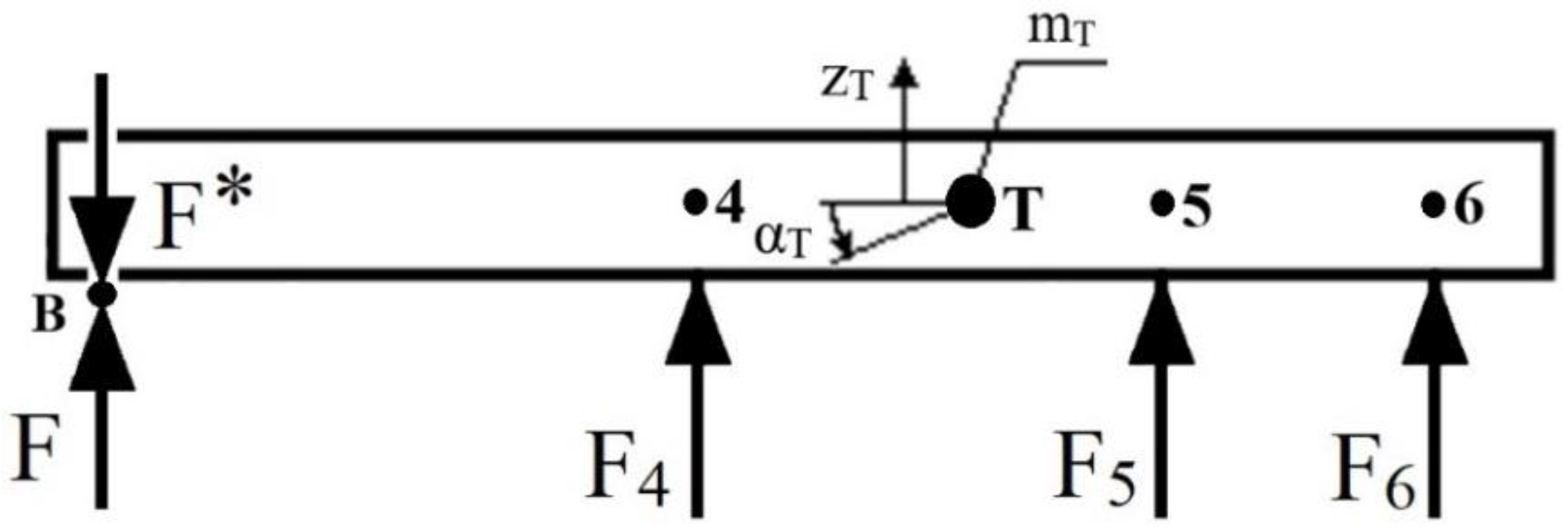
Figure 6 shows the schematic diagram used to calculate the vertical force F on the joint between the tractor’s fifth wheel and the kingpin of the semitrailer.
The form of Equations (58)–(61) indicates that the transmittance of the force F (62) is a linear combination of the transmittances (i.e., six-input ones calculated with respect to ζ1) of the quantities z4, z5, z6, z14, z15, z16, their first derivatives with respect to time and the second time derivative of zT.
F = m T · z ¨ T F 4 F 5 F 6
F 4 = k 4 · ( z 14 z 4 ) +   c 4 · ( z ˙ 14 z ˙ 4 )
F 5 = k 5 · ( z 15 z 5 ) +   c 5 · ( z ˙ 15 z ˙ 5 )
F 6 = k 6 · ( z 16 z 6 ) +   c 6 · ( z ˙ 16 z ˙ 6 )
H F ( i · ω ) = f ( H z 4 ,   H z 5 ,   H z 6 ,   H z 14 ,   H z 15 ,   H z 16 ,   H z ˙ 4 ,   H z ˙ 5 ,   H z ˙ 6 ,   H z ˙ 14 , H z ˙ 15 ,   H z ˙ 16 ,   H z ¨ T

3.2.8. Description of the Random Input from Uneven Road Surface

According to the assumptions adopted, the road profile is a realization of a stationary, Gaussian (normal) random process. The relevant ISO standards [27,28] provide a number of classes of road profile roughness, from A to H, i.e., from very good (A), through good (B), average (C), poor (D), to very poor (E and further, i.e., F, G, and H). The road of a given class is described in the ISO standard [27,28] as a function of the power spectral density Sd(Ω) [m3/rad] of a single longitudinal trace parallel to the road axis:
Sd(Ω) = Sd0)·(Ω/Ω0)−w [m3/rad]
where Ω = 2π/L is the angular frequency of the longitudinal road profile (or, in brief, angular road frequency, also referred to as “angular wave number”), [rad/m]; L is the road roughness wavelength, [m]; Ω0 is the reference road frequency (most common Ω0 = 1.0), [1/m]; Sd0) is the road roughness indicator, indicating the road pavement condition (whether it is generally good or poor), [m3/rad], and w is the road waviness indicator, indicating whether the spectrum is dominated by short or long waves, [-].
In the said ISO standard [27,28], roads of different classes differ in the Sd0) parameter. The exponent w has a constant value of w = 2. Figure 7 shows the power spectral densities of random road roughness profiles according to the ISO classification [27,28] in a two-logarithmic scale for various forms of the independent variable. As stated in the assumptions, it was assumed that the wavelength values L range from 0.1 m to 100 m. This is referred to as road roughness microprofile [2,7,8,15,23,24,25].

3.2.9. Smoothing Properties of the Tire

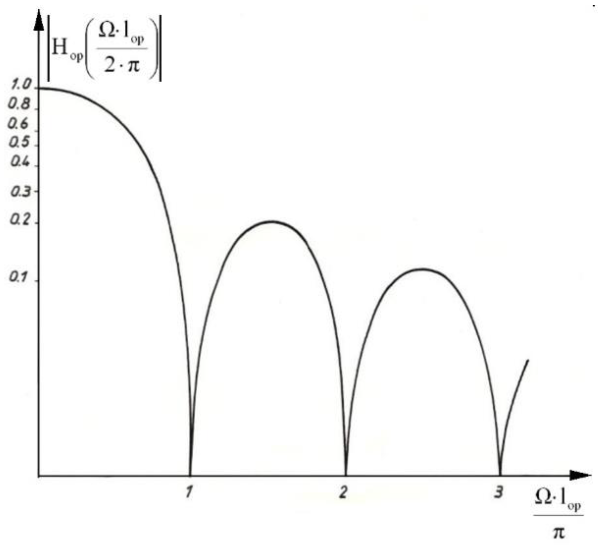
In the pneumatic tire wheel model, the “point contact model” is usually employed for the radial direction [2,6,7,8,15,16,23,24,25]. The road roughness wavelength taken into account must therefore be limited from below. The smoothing properties of the tire can be considered using a “fixed footprint tire model” [17,19] (averaging the road profile height over the length of the tire footprint) by filtering the spectra of the road profile. A filter with the following transmittance module was used [17,19]:
|Hop(Ω)| = |sin(Ω·lop)/(Ω lop)| [-]
where lop is half of the length of the footprint (i.e., tire-road interaction area) on an even horizontal road surface under static load conditions, [m].
Figure 8 shows the transmittance module of the filter representing the smoothing properties of the tire, corresponding to the “fixed footprint tire model” (FFTM). Equation (65) is a formal description of the said filtration, leading to the use of the power spectral density of the road roughness Sdf(Ω) and taking into account the smoothing properties of the tire.
Sdf(Ω) = |Hop(Ω)|2 Sd(Ω) [m3/rad]
The introduction of Sdf(Ω), i.e., the filtration effect, as the excitation enables the use of the point contact model of the tire-road interaction in the calculations [2,6,7,8,15,16,23,24,25].
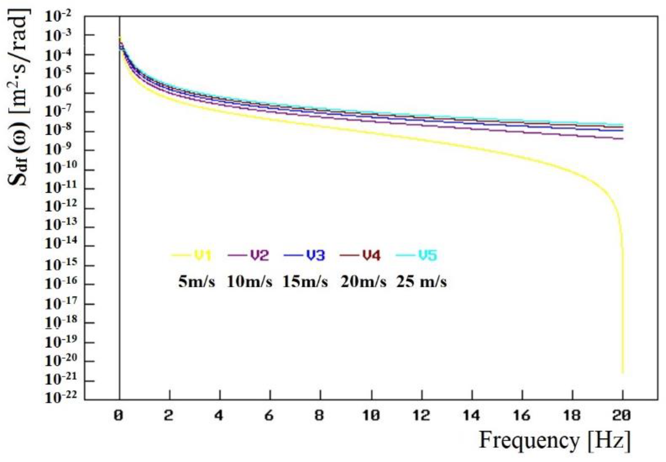
The transition from Sdf(Ω) [m3/rad] to Sdf(ω) [m2·s/rad], i.e., the change of the independent variable from Ω [rad/m] (angular road frequency) to the radian frequency ω [rad/s] requires the multiplying of Ω by the movement speed v [m/s] and simultaneous dividing of Sdf(Ω) by v [m/s].
{ ω = Ω · v           [ rad s ]                                                       S df ( ω ) = 1 v S df ( Ω = ω v )           [ m 2 · s rad ]
As a result, the definite integrals of Sdf(Ω) and Sdf(ω) in the Ω and ω bands under consideration (corresponding to each other) have the same value, i.e., the variance of the road profile height ( σ ζ 2 ) .

3.2.10. Power Spectral Density of the System Response

Due to the assumptions made (what is meant here is mainly the adopting of the excitation as having the form of a Gaussian stationary random process, linearity of the system, and V = const), the power spectral density of the system response is the product of the power spectral density of the excitation and the squared spectral transmittance module of the given output quantity [2,6,7,8,9,15,16,17,19,20,21,22,23,25,29,30,31,32]. For the estimated vertical force F on the connection between tractor’s fifth wheel and semitrailer’s kingpin, the power spectral density is expressed by Formula (67).
S F ( ω ) = | H F ( i · ω ) | 2 · S df ( ω ) [ N 2 · s / rad ]

3.2.11. Standard Deviation and Extreme Values of the System Response

The definite integrals of SF(ω) in the ω frequency band observed are the variance of the vertical force F on the joint between the tractor’s fifth wheel and the semitrailer’s kingpin ( σ F 2 ), and the square root of the variance is the standard deviation of this force ( σ F ) [2,6,7,8,9,15,19,32].
σ F = 0 ω max S F ( ω ) · d ω = 0 ω max | H F ( i · ω ) | 2 · S df ( ω ) · d ω   [ N ]
Since the system under consideration is linear and the input is a Gaussian (normal) process, the response is also a Gaussian (normal) process. For the Gaussian (normal) distribution of the force F, Equations (69) and (70) hold:
Δ Fmax / min = ± 3 · σ F   [ N ]  
F max / min = F stat ± 3 · σ F [ N ]  
where Fstat is the static load on the connection between the tractor’s fifth wheel and the semitrailer’s kingpin.

3.2.12. Natural Frequencies of the System Tested

Equation (37), if the excitation and damping are disregarded, takes the form (71), where 0 is a vector with zero components.
M · q ¨ + K · q = 0  
The solving of the ω frequency Equation (72) gives us the natural frequencies of the system [15,33], i.e., ωi [rad/s], i = 1,2, …, 9.
| K ω 2 · M | = 0
The values of the Hertz natural frequency of the system, i.e., fi [Hz], where i = 1,2, …,9, may be found from Relation (73).
f i = ω i 2 · π   Hz ]

3.2.13. Generating the Realization of a Random Process That Is the Response of the System under Analysis in the Time Domain

The response of the system under analysis in the frequency domain is the power spectral density of the vertical force F on the joint between the tractor’s fifth wheel and the semitrailer’s kingpin. It is expressed by Formula (67). To generate a realization of the system time-domain response, the Inverse Discrete Fourier Transform may be used. The algorithm known as Fast Fourier Transform (FFT) is an effective tool. The author used J. Pokorski’s subroutines presented in the publication [15].

4. Example Calculation Results

4.1. The Data Adopted for the Model of the Tractor-Semitrailer Combination

The data adopted correspond to the typical construction of a tractor-semitrailer combination found in Europe. Inertial parameters: mS = 5470 kg, mT = 25,035 kg, IS = 10,500 kg∙m2, IT = 244,800 kg∙m2, m11 = 430 kg, m12 = 1100 kg, m13 = 1100 kg, m14 = 600 kg, m15 = 600 kg, m16 = 600 kg. Suspension stiffness values: k1 = 411,800 N/m, k2 = 715,550 N/m, k3 = 715,550 N/m, k4 = 385,140 N/m, k5 = 385,140 N/m, k6 = 385,140 N/m. Values of the radial stiffness of successive pairs of road wheels: k11 = 2,140,000 N/m, k12 = 4,542,000 N/m, k13 = 4,542,000 N/m, k14 = 250,000 N/m, k15 = 250,000 N/m, k16 = 250,000 N/m. Suspension viscous damping coefficients: c1 = 23,225 N∙s/m, c2 = 52,560 N∙s/m, c3 = 52,560 N∙s/m, c4 = 43,440 N∙s/m, c5 = 43,440 N∙s/m, c6 = 43,440 N∙s/m. Viscous damping coefficients in the radial direction of successive pairs of road wheels: c11 = 1000 N∙s/m, c12 = 1800 N∙s/m, c13 = 1800 N∙s/m, c14 = 1200 N∙s/m, c15 = 1200 N∙s/m, c16 = 1200 N∙s/m. Horizontal distances between the highlighted points of the model: L1S = 1.502 m, LS2 = 1.798 m, L23 = 1.35 m, LSB = 2.473 m, LB4 = 4.89 m, L4T = −1.047 m, LT5 = 2.357 m, L56 = 1.31 m.
The vehicle motion was analysed for the speeds v equal to: 5 m/s, 10 m/s, 15 m/s, 20 m/s, and 25 m/s, i.e., for V equal to 18 km/h, 36 km/h, 54 km/h, 72 km/h and 90 km/h.
The length of the tire footprints under static conditions was assumed as 2·lop = 0.25 m.
Three road sections with the following values of the power spectral density parameters of the road roughness were selected for the calculations:
-
road 1: road B (good); Sd0) = 0.000004, Ω0 = 1.0, w = 2;
-
road 2: road C (average); Sd0) = 0.000016, Ω0 = 1.0, w = 2;
-
road 3: road D (poor); Sd0) = 0.000064, Ω0 = 1.0, w = 2.
The shortest road profile wavelength is L = 0.1 m and the longest one is L = 100 m.
The frequency band assumed for the analysis was 0–20 Hz (0–125.66 rad/s).

4.2. Natural Frequencies of the System under Analysis

For the data adopted, the following solution (74) of the eigenproblem within the natural frequency range assumed was obtained:
f1 = 1.28 Hz,  f2 = 1.62 Hz,  f3 = 1.95 Hz
 f4 = 11.01 Hz,  f5 = 11.02 Hz,   f6 = 11.04 Hz,
  f7 = 11.04 Hz,  f8 = 11.05 Hz,  f9 = 12.29 Hz
The first three frequencies can be associated with the vertical (and, consequently, also angular) movement of the vehicle combination body solids (q1 = z1, q2 = z2, q3 = zT). The other six frequencies are related to the movement of the unsprung masses of the tractor unit and the semitrailer (q4 = z11, q5 = z12, q6 = z13, q7 = z14, q8 = z15, q9 = z16).

4.3. Power Spectral Densities of the Random Excitation due to Road Surface Irregularities, for the Adopted Speed Values of the Vehicle Combination Tested

For the road of a given type and the vehicle under consideration (the lop is meant here), the power spectral density of the input Sdf(Ω) [m3/rad] in the domain of Ω [rad/m] (angular road frequency) is constant (see (63) and (65)). The transition to the independent variable in the form of radian frequency ω [rad/s] involves the adopting of a vehicle combination speed v [m/s] different from 1 m/s (we are talking only about the calculation side, without going into the area of analysis as such and into the units of the quantities described). The form of the power spectral density function of the excitation Sdf(ω) [m2·s/rad] changes. It depends on the speed v of movement of the combination tested, which is described by Relation (66).
Figure 9 shows (on a semi-logarithmic scale) examples of the power spectral density function of the excitation Sdf(ω) for road C (average) and the five vehicle speed values v considered: 5 m/s, 10 m/s, 15 m/s, 20 m/s, and 25 m/s.
As the speed increases, the value of the power spectral density increases too, which results from the fact that a given frequency f [Hz] (and thus the radian frequency ω [rad/s]) corresponds, with the growth of speed v, to an increasingly longer wave L (and, in consequence, decreasing angular road frequency Ω [rad/m])—see Figure 7 and the description of Equation (63). For the lowest speed v = 5 m/s, the tire filtration effect (averaging the road profile height over the length of the tire footprint) is visible when the “fixed footprint tire model” (FFTM) is used—see Equations (64) and (65) and Figure 8. Short road roughness wavelengths, comparable to the footprint length 2∙lop, translate into kinematic excitation with frequencies being within the range under consideration, i.e., 0–20 Hz.

4.4. Modules of Transmittance of the Vertical Force F on the Joint between Tractor’s Fifth Wheel and Semitrailer’s Kingpin

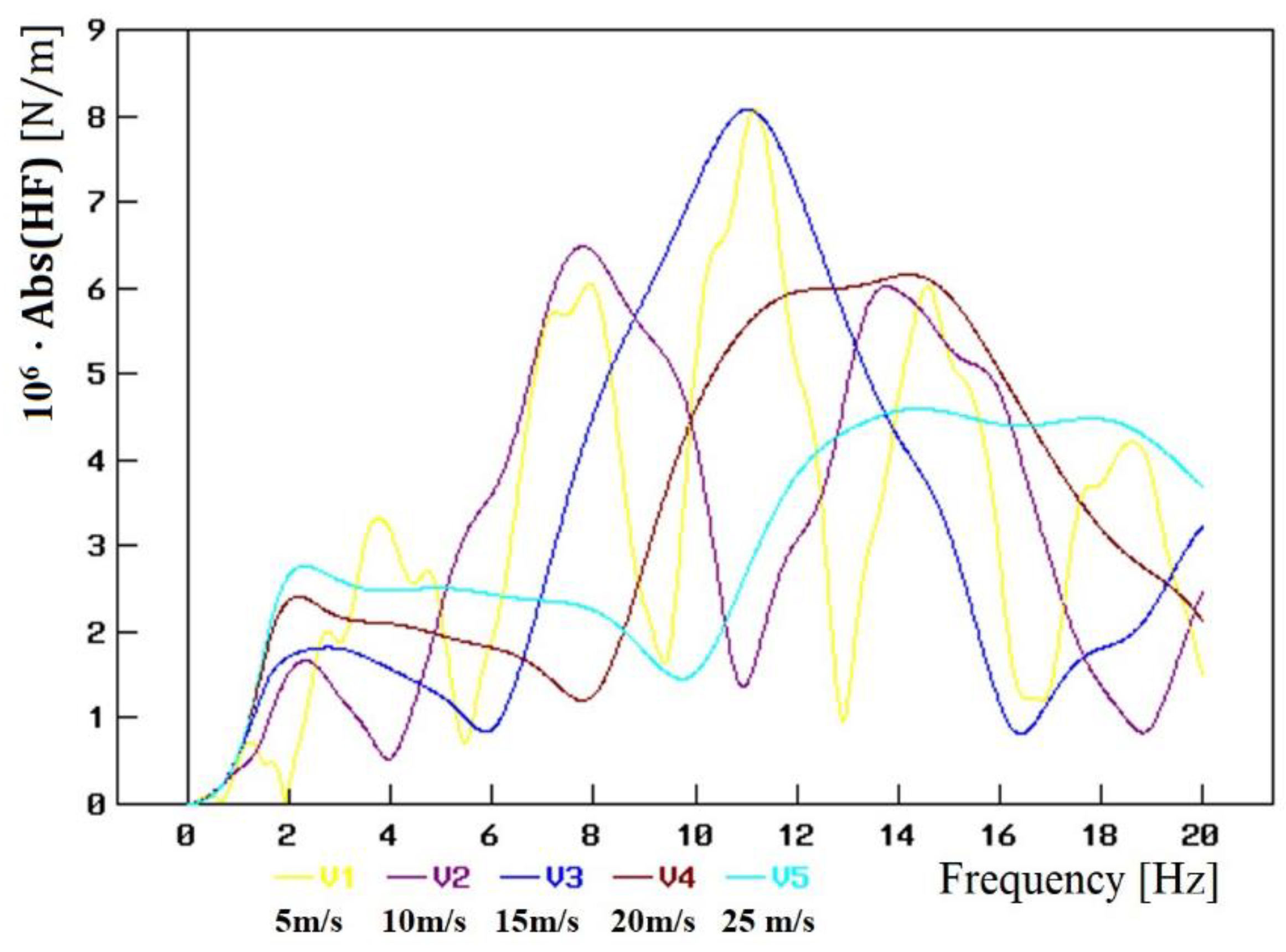
The transmittance HF(i∙ω) of the force F on the joint between the tractor’s fifth wheel and the semitrailer’s kingpin is a linear combination of the transmittances (i.e., six-input ones calculated with respect to ζ1) of the quantities z4, z5, z6, z14, z15, z16, their first derivatives with respect to time, and the second time derivative of zT, which is described by Equation (62). Figure 10 shows the modules of this transmittance for the five-speed values v considered: 5 m/s, 10 m/s, 15 m/s, 20 m/s, and 25 m/s.
Attention is drawn to the high values of the modules of this transmittance for all of the five speeds of movement of the vehicle combination. The higher the speed, the fewer maximums of the transmittance analysed. However, their values remain at a similar level. It should be reminded here that the influence of the vehicle speed manifests itself in changes in phase shifts of the kinematic excitations, which is described by Equations (26)–(30), (49)–(53), and (54)–(57). The influence of the natural frequencies of the system is less visible (74). However, polyharmonic components appear for the first three of them.

4.5. Power Spectral Densities of the Vertical Force F on the Joint between the Tractor’s Fifth Wheel and the Semitrailer’s Kingpin, for the Assumed Values of Speed of the Vehicle Combination under Analysis

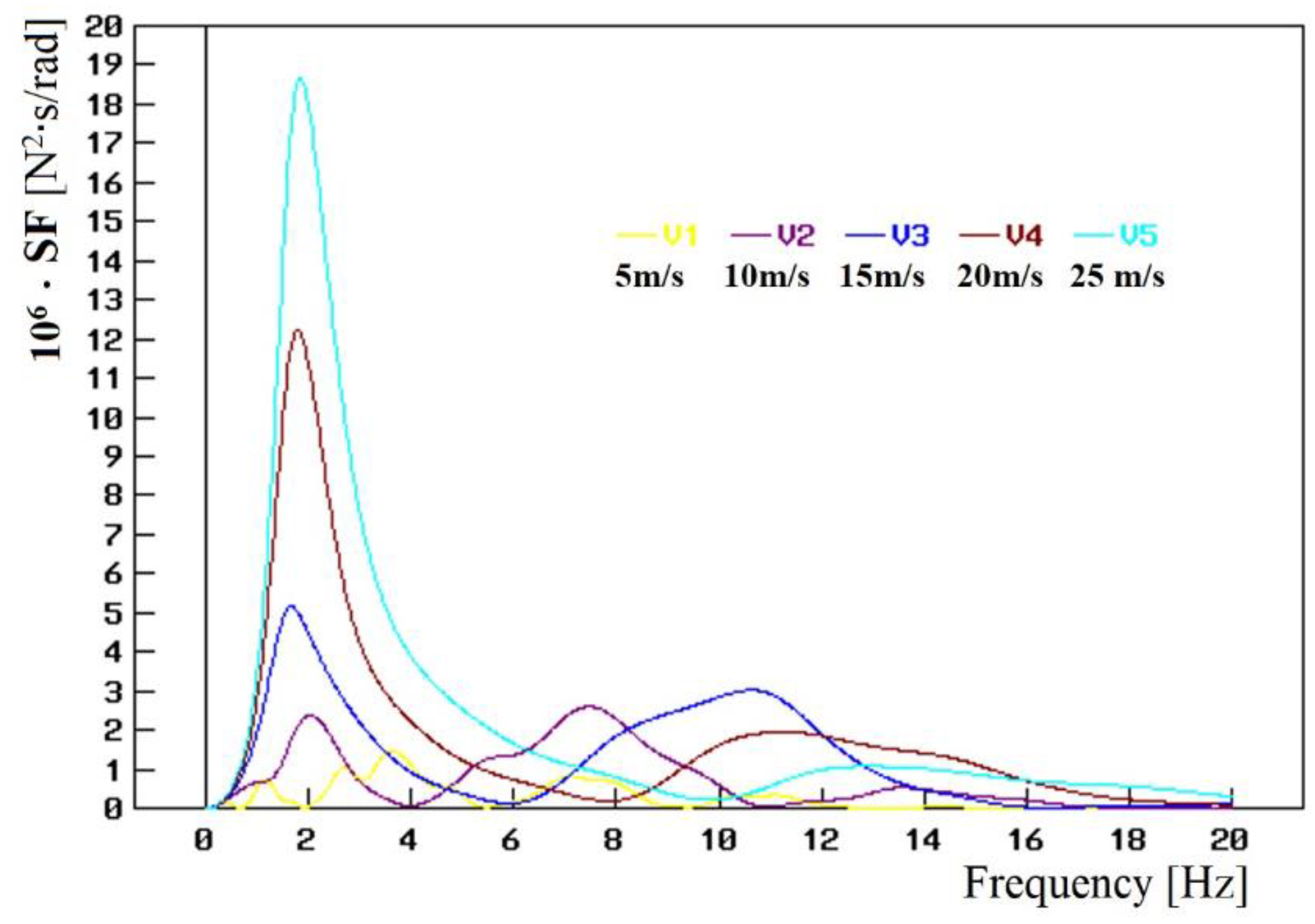
The spectral density of the linear system response is the product of the power spectral density of the input and the squared spectral transmittance module of a given output quantity. In the case of the vertical force F acting on the connection between the tractor’s fifth wheel and the kingpin of a semitrailer, this is expressed by the SF(ω) Formula (67). Figure 11 shows the SF(ω) function for road C (average) and the five vehicle movement speeds v taken into account, i.e., 5 m/s, 10 m/s, 15 m/s, 20 m/s, and 25 m/s.
The value of the power spectral density SF(ω) [N2∙s/rad] of the vertical force F [N] on the connection between the tractor’s fifth wheel and the semitrailer’s kingpin is influenced by the transmittance module of this quantity ǀHF(i∙ω)ǀ [N/m] (and here the impact of the vehicle speed manifests itself in changes in phase shifts of the kinematic excitations, which is described by Equations (26)–(30), (49)–(53), and (54)–(57)) and by the value of the power spectral density of the kinematic excitation due to road surface irregularities Sdf(ω) [m2·s/rad], the dependence of which on the vehicle speed is shown in Figure 9. In this case, the influence of the natural frequencies of the system (74), especially of the first three of them, is clearly visible.

4.6. Extreme Values of the Dynamic Force Components on the Joint between the Tractor’s Fifth Wheel and the Semitrailer’s Kingpin

As already mentioned, the definite integrals of SF(ω) [N2∙s/rad] in the frequency band ω [rad/s] observed (i.e., in the corresponding Hertz frequency f [Hz] band as well) are the variance of the vertical force F [N] on the joint between the tractor’s fifth wheel and the semitrailer’s kingpin ( σ F   2 [N2]) and the square root of the variance is the standard deviation of this force ( σ F [N]). It should be noted that this is the dynamic component of this force, in which the static load is not taken into account. Since the system tested is linear and the input is a Gaussian (normal) process, the response is also a Gaussian (normal) process. For the Gaussian (normal) distribution, the extreme values of the force F are treble σ F , which is described by Equation (69).
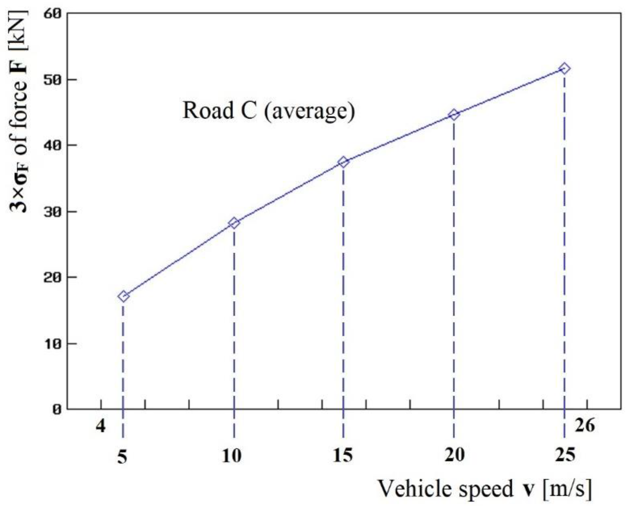
Figure 12 shows the values of 3× σ F   [N] of the dynamic component of the vertical force F [N] on the connection between the tractor’s fifth wheel and the kingpin of the semitrailer, for road C (average) and the five vehicle motion speeds v considered: 5 m/s, 10 m/s, 15 m/s, 20 m/s, and 25 m/s. They make a result of the integration of SF(ω) [N2∙s/rad] in the frequency band ω [rad/s] (and, therefore, also the Hertz frequency band f [Hz]) observed.
There is a clear upward trend in the extreme value of the dynamic vertical force on the connection between the tractor’s fifth wheel and the kingpin of the semitrailer with increasing vehicle movement speed.

4.7. Realization of the Random Process That Describes the Dynamic Component of the Vertical Force F on the Joint between the Tractor’s Fifth Wheel and the Kingpin of the Semitrailer

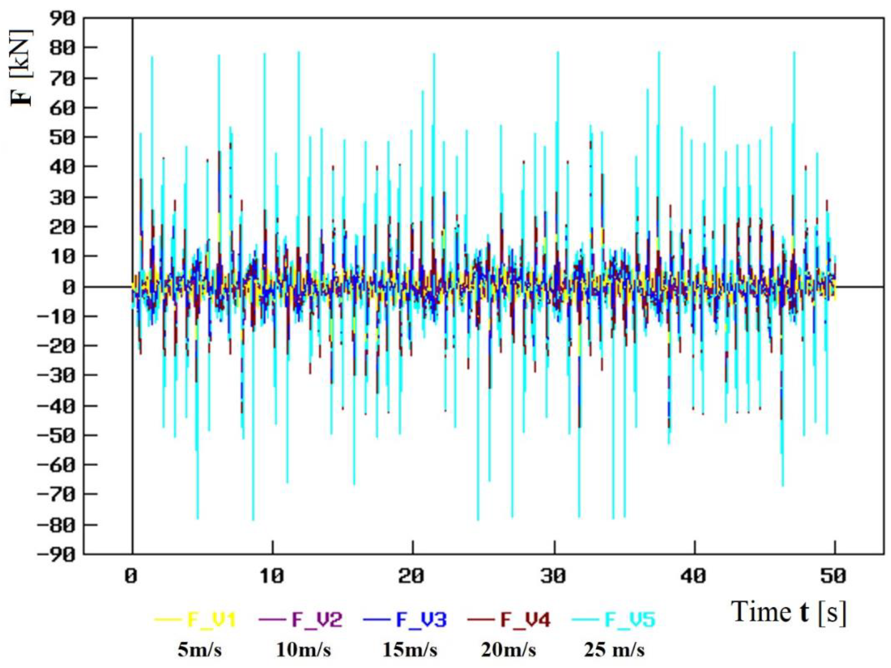
What is sought at first is the response of the system under analysis, i.e., the dynamic component of the vertical force F on the joint between the tractor’s fifth wheel and the semitrailer’s kingpin. When the operating loads on the vehicle’s structural nodes are examined by simulation on laboratory test stands, time realizations of such a force must be applied as an input. In our case, the said input is the F(t) waveform generated using the inverse discrete Fourier transform.
Figure 13 shows example waveforms generated to represent the force F(t) for road C (average) and the five vehicle speed values v considered: 5 m/s, 10 m/s, 15 m/s, 20 m/s, and 25 m/s. The curves make a realization whose length (duration time) is 51.24997 ≈ 51.25 s. The realization of this type (after adding a static component) may be used as input during the simulation tests carried out on laboratory test stands to examine the operating loads on the tractor’s fifth wheel as well as the semitrailer’s kingpin.
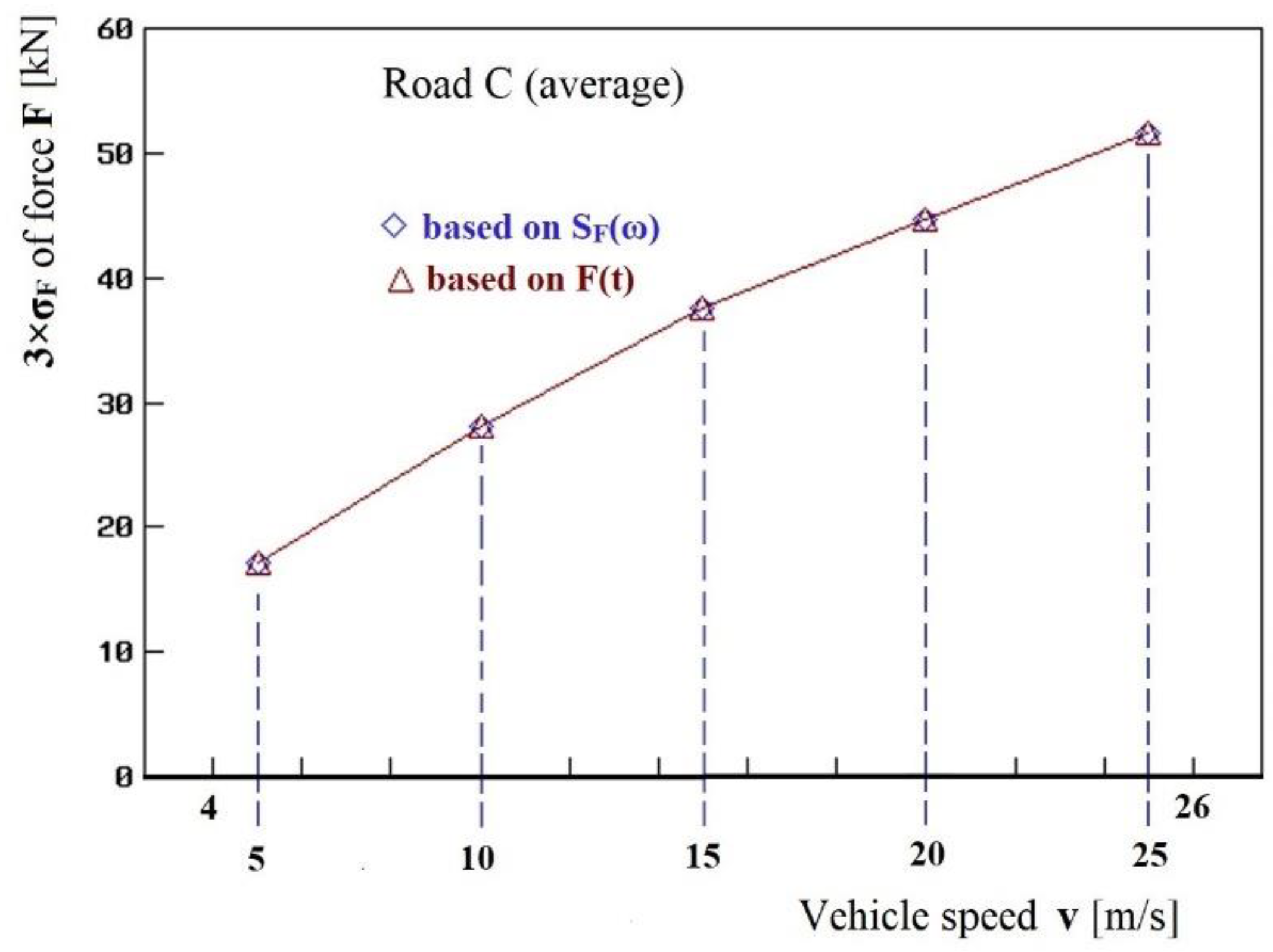
Figure 14 shows the calculation results for road C (average) and the five vehicle speed values v considered: 5 m/s, 10 m/s, 15 m/s, 20 m/s, and 25 m/s. This is a comparison of the values of 3 × σ F of the dynamic component of the vertical force F on the joint between the tractor’s fifth wheel and the kingpin of the semitrailer, obtained (see Figure 12) from the frequency analysis (as a result of the integration of SF(ω) [N2∙s/rad] in the frequency band ω [rad/s] observed and, therefore, in the corresponding Hertz frequency f [Hz] band as well) and those calculated on the grounds of the generated realization of F(t) (based on the results presented in Figure 13). The differences between these results are so small that they are practically invisible in Figure 14. This shows that the calculations presented are correct.

5. Summary, Final Conclusions

The author has presented a proposal to use the simulation and modelling for determining the input (excitation) to be applied when testing a motor vehicle’s structural components (component units, subassemblies, and individual parts) without the need to test the complete vehicle. In addition to the general concept, he presented an example of the procedure for determining the spectrum and time history of the load on a selected vehicle’s structural node to be used in durability tests. He used the physical and mathematical model of the tractor-semitrailer combination.
He determined the power spectral densities of the random excitation due to road surface irregularities for the adopted speed values of the vehicle tested. He calculated the transmittance modules and the power spectral densities of the vertical force on the joint between the tractor’s fifth wheel and the semitrailer’s kingpin and the extreme values of the dynamic components of this force. By applying the inverse discrete Fourier transform, he generated realizations of the said force, suitable for durability tests. The limitation of the work scope to the testing of a specific structural node of interest reduces the scope of the research process and its costs. The use of a linear model enables qualitative and quantitative analysis, which is a significant advantage of this method.
Its disadvantage is the impossibility of taking into account the non-linearities that occur in real vehicle designs and are related to the characteristics of suspension (non-linearity of the elasticity curves, the influence of the suspension travel limiters for the compression and rebound phases, dry friction), and tires (regarding the movements in the radial direction, e.g., non-linearity of the elasticity curves, wheel hops, etc.). It is also not possible (for formal reasons) to perform a direct frequency analysis of the longitudinal force component on the joint between the tractor’s fifth wheel and the semitrailer’s kingpin, analogous to the one having been presented.
To eliminate these inconveniences, it is possible to build a similar model, which would make it possible to take into account the non-linearities mentioned above and would be adapted for the analysis of the dynamics of the tractor-semitrailer combination in the time domain. A drawback of such a solution, however, is a significant extension of the time of simulation calculations and the necessity for secondary qualitative and quantitative analysis. Nevertheless, the argument of limiting the scope of tests to a specific structural node of interest to us will still be valid, and this will reduce the scope and costs of the work. This is important for both traditional vehicle designs and electric and hybrid ones.

Funding

This research received no external funding. Is based on work at the author’s affiliation institutions.

Institutional Review Board Statement

Not applicable.

Informed Consent Statement

Not applicable.

Data Availability Statement

Not applicable.

Conflicts of Interest

The author declares no conflict of interest.

References

  1. Azrulhisham, E.; Asri, Y.M.; Dzuraidah, A.W.; Nik Abdullah, N.M.; Che Hassan, C.H.; Shahrom, A. Application of road simulator service loads in automotive component durability assessment. Open Ind. Manuf. Eng. J. 2011, 4, 1–7. [Google Scholar] [CrossRef] [Green Version]
  2. Dukkipati, R.; Pang, J.; Qatu, M.S.; Sheng, G.; Shuguang, Z. Road Vehicle Dynamics; SAE International: Warrendale, PA, USA, 2008. [Google Scholar]
  3. Gierulski, W. Kształtowanie drgań w stanowiskowych badaniach symulacyjnych. Zesz. Nauk. Politech. Świętokrzyskiej Mech. 1991, 46. [Google Scholar]
  4. Kaczor, M.; Januszka, M. Optymalizacja konstrukcji naczep z zastosowaniem symulatora drogi MTS. Mechanik 2019, 92, 52–54. [Google Scholar] [CrossRef]
  5. MTS. Model 320 Tire-Coupled Road Simulators. Versatile, Repeatable Road Simulation for the Full Range of Vehicle Sizes and Applications. MTS Booklet. Available online: https://www.mts.com/cs/groups/public/documents/library/dev_002219.pdf (accessed on 1 February 2020).
  6. Osiecki, J.W. Badania Pojazdów Samochodowych i ich Zespołów na Stanowiskach Badawczych; Specjalne zagadnienia mechaniki i sterowania; Politechnika Świętokrzyska: Kielce, Poland, 2004; pp. 19–49. ISBN 83-88906-16-x. [Google Scholar]
  7. Osiecki, J.W.; Gromadowski, T.; Stępiński, B. Badania Pojazdów Samochodowych i ich Zespołów na Symulacyjnych Stanowiskach Badawczych; Wydawnictwo Instytutu Technologii Eksploatacji—PIB: Radom, Poland, 2006; ISBN 83-7204-510-0. [Google Scholar]
  8. Rao, S.S. Mechanical Vibrations, 5th ed.; Prentice Hall—Pearson: Hoboken, NJ, USA, 2010; ISBN 978-0-13-212819-3. [Google Scholar]
  9. Rill, G.; Castro, A.A. Road Vehicle Dynamics. Fundamentals and Modeling with MATLAB®, 2nd ed.; CRC Press: Boca Raton, FL, USA; Taylor & Francis Group: Abingdon, UK, 2020; ISBN 9780367199739. [Google Scholar]
  10. Homepage of Łukasiewicz PIMOT. BLY Laboratory. Available online: https://pimot.lukasiewicz.gov.pl/index.php?option=com_content&view=article&id=40&Itemid=222 (accessed on 7 October 2022).
  11. Homepage of MTS. Available online: https://test.mts.com/industries/automotive (accessed on 13 May 2020).
  12. Homepage of Wielton. Available online: https://wieltongroup.com/innowacyjnosc/ (accessed on 10 September 2022).
  13. Homepage 40ton.net (Motoryzacja dla Profesjonalistów—Automotive for Professionals). Available online: https://40ton.net/zobacz-jak-dziala-i-do-czego-sluzy-centrum-badawczo-rozwojowe-firmy-wielton-otwarte-wczoraj-w-wieluniu/ (accessed on 10 September 2022).
  14. Lozia, Z. The concept of the application of modelling and simulation to simplify and reduce the cost of durability tests of vehicles and their components. In IOP Conference Series: Materials Science and Engineering; IOP Publishing: Bristol, UK, 2022; Volume 1247. [Google Scholar] [CrossRef]
  15. Kamiński, E.; Pokorski, J. Teoria Samochodu. Dynamika Zawieszeń i Układów Napędowych Pojazdów Samochodowych; WKŁ: Warsaw, Poland, 1983. [Google Scholar]
  16. Kasprzyk, T.; Prochowski, L. Teoria Samochodu. Obciążenia Dynamiczne Zawieszeń; WKŁ: Waraw, Poland, 1990. [Google Scholar]
  17. Lozia, Z. Analiza Ruchu Samochodu Dwuosiowego na tle Modelowania jego Dynamiki; Monograph 41; Transport; Prace Naukowe Politechniki Warszawskiej: Warsaw, Poland, 1998. [Google Scholar]
  18. Lozia, Z. Examples of authorial models for the simulation of motor vehicle motion and dynamics. Zesz. Nauk. Inst. Pojazdów PW 2015, 104, 9–27. [Google Scholar]
  19. Lozia, Z. The use of a linear quarter-car model to optimize the damping in a passive automotive suspension system—A follow-on from many authors’ works of the recent 40 years. Arch. Automot. Eng.—Arch. Motoryz. 2016, 71, 39–71. [Google Scholar] [CrossRef]
  20. Osiecki, J. Dynamika Maszyn; Wojskowa Akademia Techniczna: Warsaw, Poland, 1994. [Google Scholar]
  21. Osiński, Z. Teoria Drgań; PWN: Warsaw, Poland, 1978. [Google Scholar]
  22. Prochowski, L. Pojazdy Samochodowe. Mechanika Ruchu; WKŁ: Warsaw, Poland, 2005. [Google Scholar]
  23. Arczyński, S. Mechanika Ruchu Samochodu; WNT: Warsaw, Poland, 1993. [Google Scholar]
  24. Mitschke, M. Teoria Samochodu. Dynamika Samochodu; WKŁ: Warsaw, Poland, 1977. [Google Scholar]
  25. Mitschke, M. Dynamika Samochodu; Tome 2: Drgania; WKŁ: Warsaw, Poland, 1989. [Google Scholar]
  26. Lozia, Z. Simulation testing of two ways of disturbing the motion of a motor vehicle entering a skid pad as used for tests at Driver Improvement Centres. Arch. Automot. Eng.—Arch. Motoryz. 2016, 72, 111–125. [Google Scholar] [CrossRef]
  27. ISO/TC 108/253; Reporting Vertical Road Surface Irregularities. Generalised Vertical Road Inputs to Vehicles. ISO: Geneva, Switzerland, 1980.
  28. ISO 8608:2016(E); 2nd ed. Mechanical Vibration—Road Surface Profiles—Reporting of Measured Data. ISO: Geneva, Switzerland, 2016.
  29. Meirovitch, L. Elements of Vibration Analysis; McGraw-Hill Kogakusha: Tokyo, Japan, 1975. [Google Scholar]
  30. Meirovitch, L. Fundamentals of Vibrations; McGraw-Hill International Edition: Singapore, 2001. [Google Scholar]
  31. Newland, D.E. An Introduction to Random Vibration Spectral and Wavelet Analysis, 3rd ed.; Dover Publications, Inc.: Mineola, NY, USA, 1993. [Google Scholar]
  32. Osiecki, J. Podstawy Analizy Drgań Mechanicznych; Politechnika Świętokrzyska: Kielce, Poland, 1979. [Google Scholar]
  33. Bishop, R.E.D.; Gladwell, S.M.L.; Michaelson, S. Macierzowa Analiza Drgań; WNT: Warsaw, Poland, 1972. [Google Scholar]
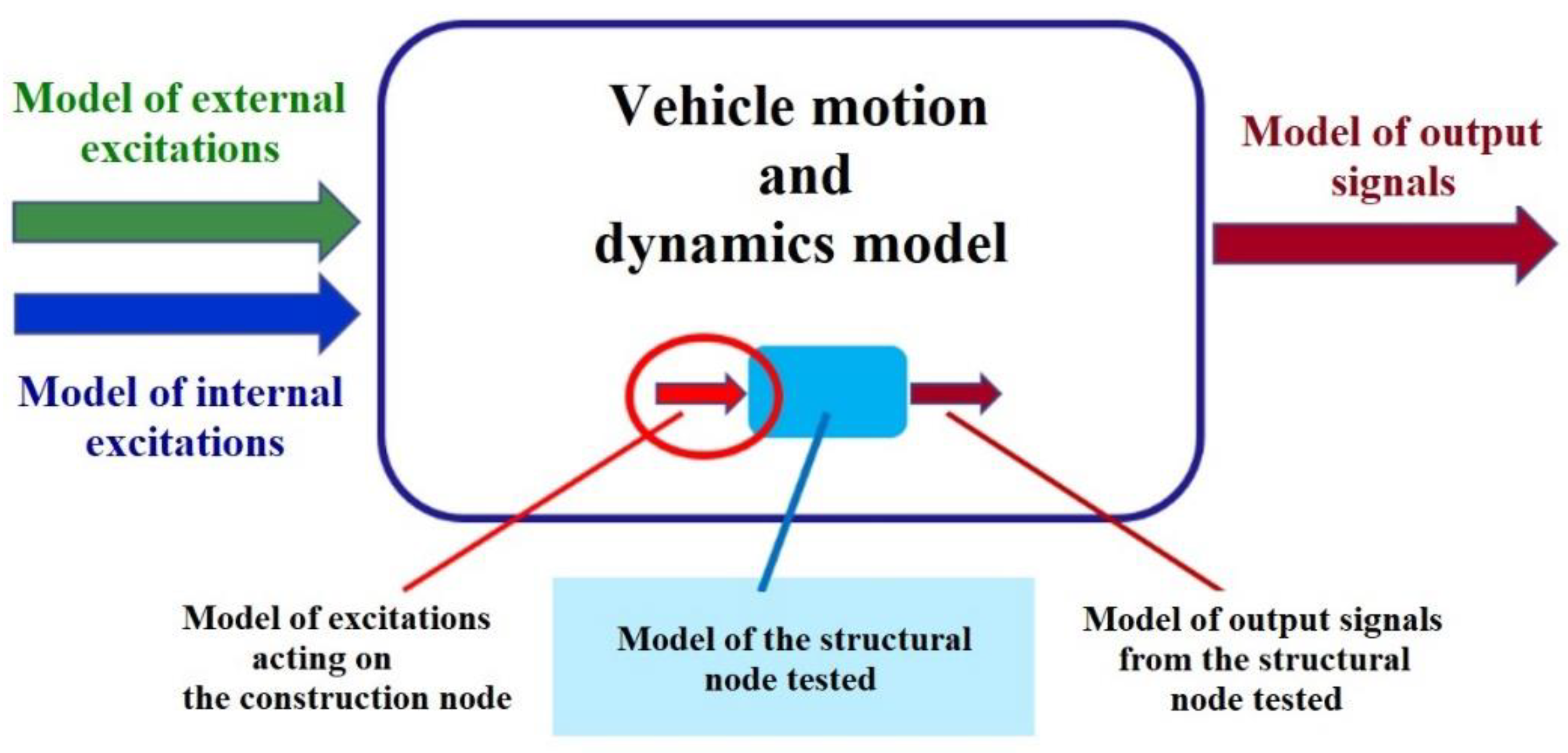
Figure 2. Determining the forces that act on the tested node of the vehicle structure (the drawing has been based on the author’s own drawing presented in the publication [14]).
Energies 15 09398 g002
Figure 3. Determining of the excitations that act on the vehicle construction node under test, by means of digital simulation of the working processes that accompany the vehicle movement (the drawing has been based on author’s own drawing presented in publications [14,18]).
Energies 15 09398 g003
Figure 4. Tractor-semitrailer combination in a straight-line motion with a constant speed V. The structural node tested is the connection between tractor’s fifth wheel and the kingpin of the semitrailer.
Energies 15 09398 g004
Figure 5. The physical model of the tractor-semitrailer combination in a rectilinear motion with a constant speed V (for descriptions of the model components see the text).
Energies 15 09398 g005
Figure 6. Diagram used to calculate the vertical force F on the joint between the tractor’s fifth wheel and the kingpin of the semitrailer. F is the force exerted by the fifth wheel on the semitrailer and F* = −F is the force exerted by the semitrailer on the fifth wheel.
Energies 15 09398 g006
Figure 7. Power spectral densities of random road roughness profiles according to the ISO classification (based on [27,28]): from A to H. Two-logarithmic scale. The meaning of the lowercase letters in the picture: a—power spectral density Sd(1/L) [m3]; b—power spectral density Sd(Ω) [m3/rad]; c—wavelength L [m]; d—wavenumber 1/L [1/m]; e—angular wave number of the road (i.e., angular road frequency) Ω = 2π/L [rad/m].
Energies 15 09398 g007
Figure 8. The transmittance module of the filter representing the smoothing properties of the tire, corresponding to the “fixed footprint tire model” (FFTM) [17,19] (for the notation used see the text).
Energies 15 09398 g008
Figure 9. Power spectral density of the excitation Sdf(ω) for road C (average) and five vehicle speed values v: 5 m/s, 10 m/s, 15 m/s, 20 m/s, and 25 m/s.
Energies 15 09398 g009
Figure 10. Modules of transmittance HF(i∙ω) of the force F on the joint between the tractor’s fifth wheel and semitrailer’s kingpin for the five-speed values v considered: 5 m/s, 10 m/s, 15 m/s, 20 m/s, and 25 m/s.
Energies 15 09398 g010
Figure 11. Power spectral density SF(ω) of the force F on the connection between the tractor’s fifth wheel and the semitrailer’s kingpin for road C (average) and five vehicle speeds v: 5 m/s, 10 m/s, 15 m/s, 20 m/s, and 25 m/s.
Energies 15 09398 g011
Figure 12. Values of 3× σ F of the dynamic component of the vertical force F on the connection between the tractor’s fifth wheel and the semitrailer’s kingpin, for road C (average) and the five vehicle movement speeds v taken into account, i.e., 5 m/s, 10 m/s, 15 m/s, 20 m/s, and 25 m/s.
Energies 15 09398 g012
Figure 13. The complete realization of the input F(t), i.e., the dynamic component of the vertical force on the connection between the tractor’s fifth wheel and the kingpin of the semitrailer, for road C (average) and the five vehicle speed values v considered: 5 m/s, 10 m/s, 15 m/s, 20 m/s, and 25 m/s.
Energies 15 09398 g013
Figure 14. Values of 3× σ F of the dynamic component of the vertical force on the connection between the tractor’s fifth wheel and the kingpin of the semitrailer, for road C (average) and the five vehicle speed values v considered, i.e., 5 m/s, 10 m/s, 15 m/s, 20 m/s, and 25 m/s. Comparison of the results obtained from the frequency analysis and those calculated on the grounds of the generated realization of F(t).
Energies 15 09398 g014
Publisher’s Note: MDPI stays neutral with regard to jurisdictional claims in published maps and institutional affiliations.