Abstract
The flow ripple in an internal gear pump was measured by means of a new instantaneous high-pressure flowmeter. The flowmeter consists of two pressure sensors mounted on a piece of the straight steel pump delivery line, and a variable-diameter orifice was installed along such a line, downstream of the flowmeter, to generate a variable load. Three distinct configurations of the high-pressure flowmeter, characterized by a different distance between the pressure transducers, were analyzed. Furthermore, a comprehensive fluid dynamic 3D model of the pump and of its high-pressure delivery line was developed and validated in terms of both the delivery pressure and the flow ripple for different pump working conditions. For the three examined configurations of the flowmeter, the measured flowrate time histories matched the corresponding numerical distributions at the various operating points. Finally, the validated 3D model was applied to predict the incomplete filling working of the interteeth chambers, and the obtained numerical pressure time histories along the delivery line were used, as input data, to assess the reliability of the flowmeter algorithm even in these severe operating conditions.
1. Introduction
The flow ripple is an intrinsic characteristic of almost all positive displacement pumps. It is generated by the cyclic variation of the variable volume chambers connected to the delivery side. The flow oscillation is probably the major demerit of the positive displacement machines, because its interaction with the circuit generates pressure ripples (fluid-borne noise), consequently leading to a vibration of the pump casing and of the pipeline (structure-borne noise) and finally acoustic noise (airborne noise).
In recent years, the progressive electrification of many offroad vehicles, with the hybridization of the thermal propulsion system (the electric motor is quieter than the internal combustion engine), has made the hydraulic pump become a primary source of noise of the entire vehicle. Furthermore, another general recent trend is the hybridization of the hydraulic circuits, where the flowrate to each actuator is controlled by a variable-speed electric motor that drives a small, fixed displacement pump, instead of using a centralized pump and many flow control valves [1,2,3,4]. Alternative configurations still make use of a centralized pump for supplying a constant amount of hydraulic energy, but the remaining energy for satisfying the load requirement of each actuator is generated electrically by a local pump driven by an electric motor [5,6]. Regardless of the specific layout, these new architectures require an increase in the operating speed of the pump with the risk of the phenomenon of incomplete filling. When it occurs, the real flow ripple and the noise increase significantly. Both passive and active systems can be applied to reduce the flow ripple. The former involve the exchange of flowrates between the internal volumes of the pump by means of channels or poppet valves [7,8], and the latter are based on the generation of an opposite volume variation through a quick movement of the plate for the change in the pump displacement to compensate for the ripple caused by the pump’s chambers. In axial piston pumps, studies have been performed on the effect of the swash plate oscillation [9,10] and on the use of a piezoelectric actuator [11,12,13].
In this context, considering the number of recent studies involving the optimization of fluid power pumps, an important research topic is the experimental measurement of the flow ripple for a more direct validation of the pump’s simulation models and of the actions taken for smoothing the flow irregularity. For rough analyses, the theoretical kinematic flow ripple that is calculated starting from the geometrical parameters of the pump could be used [14]. However, the shape and the amplitude of the real flowrate oscillation differ significantly from the real waveform, due to some nonidealities, namely leakages, fluid compressibility and filling factor of the chambers. Due to the difficulty in measuring directly the instantaneous flowrate at the delivery port of the pump, the common experimental procedure is the measurement of the pressure ripple that is highly dependent on the pump delivery circuit layout. Few techniques are available for the measurement of the flow ripple of positive displacement pumps. A popular technique is the secondary source method [15] that was proven to be reliable, but it requires a quite complex circuit. Other techniques need two [16,17,18] or three [19,20] high-dynamic pressure transducers mounted on a straight pipeline. Complex algorithms, based on hydraulic models, are required to obtain the flow ripple amplitudes, and these techniques can only be applied to laminar flows. A comparison between the methods presented in [17,19] can be found in [21].
In the present investigation, the measuring principle described in the paper [22] and developed for a high-pressure pipeline flow characterization, is applied to the measurement of the flow ripple for a positive displacement pump. The method is based on continuity and momentum balance flow equations and was implemented in the innovative Flotec flowmeter. The instrument had been already tested successfully to measure the instantaneous flowrate entering the injector of a Common Rail diesel injection system [23,24], for which a maximum nominal pressure of 1800 bar was reached.
Moreover, in other previous studies, the algorithm was also effectively tested on flow power components. In [25], the velocity of a high-dynamic servoactuator was used for obtaining the data for the validation of the instantaneous flow passing through an electro-hydraulic proportional valve. A different approach was followed in [26], where, at first, a simulation model of an external gear pump with its delivery line was validated, based on the experimental pressure ripple, and, then, the flowmeter was validated by means of the comparison with the simulated instantaneous flow oscillation for pressure levels up to 133 bar.
The present paper represents a further step for extending the validation range of the flowmeter. An internal gear pump was used as a reference: compared to [26], the main difference is the smaller flow ripple; in fact, the amplitude of the oscillation with respect to the mean value is one order of magnitude lower. Furthermore, the pressure range below 10 bar was investigated, whereas the pressure levels considered in [25] were even higher than 100 bar. Finally, the ability of the algorithm to measure the flowrate in conditions of incomplete filling at a high pump speed with a significant reverse flow at the delivery port and a higher frequency of the oscillation was tested.
2. Pump Description
The tested internal gear pump, manufactured by Rexroth, features a displacement of 6.5 cc/rev and a maximum working pressure of 210 bar, and the speed can vary in the 600–3600 rpm range. A photo of the pump is shown in Figure 1a, where the direction of the rotation is counterclockwise. The internal gear (driver), which is integral with the shaft, features 13 teeth and an external diameter of 37.75 mm, while the driven external gear is characterized by 20 teeth and an external diameter of 66 mm; the axial width of the gearset is 13 mm. The working fluid is transported by the interteeth volumes of both rotors, and it is delivered toward the outlet port when the teeth mesh. The fluid enters and leaves the interteeth volumes through radial holes drilled on the outer diameter of the external gear (Figure 1b). The inlet and outlet ports are connected to the holes through circumferential grooves machined on the pump casing.
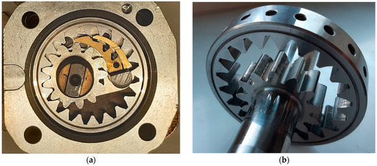
Figure 1.
Photo of the pump (a) and detail of the rotors with the radial holes (b).
The pump is provided of both axial and radial gap compensation. The former is obtained by two lateral plates that are pushed against the rotors by the delivery pressure acting on the rear side, while the latter by means of the double-floating insert (crescent). More in detail, the delivery pressure acts in the small volume between the two elements of the crescent that, in turn, are pushed against the teeth of the two gears in order to compensate the tip clearance.
3. Test Bench and Algorithm of the Flowmeter
The experimental campaign was performed at the hydraulic test bench installed at Rabotti Srl research laboratory. The pump was installed in a closed circuit, and a variable-speed electric motor was employed to drive it. The pump delivery line consists of a 710 mm long straight pipe where, at the extremity, a variable orifice was installed to manually change the pump load; the pipe diameter d is equal to 7.8 mm. Shell V-Oil ISO 4113 was used for the entire experimental campaign.
The instantaneous high-pressure flowmeter was constituted by two pressure transducers, the measurements of which are indicated with pup and pdown, installed at a certain distance in the delivery line. These transducers feature a measuring range of 0–10 bar, a nonlinearity error <±0.3% FSO and a dynamic response up to 5 kHz. The flowmeter algorithm is based on a simplified coupled solution of the mass conservation and momentum balance partial differential equations written for a one-dimensional duct [27]:
where p, and u stand for the cross-section averaged flow pressure, flow density and flow velocity, respectively; d is the pipe diameter; t represents the time; x is the spatial coordinate aligned with the duct axis, and represents the wall shear stress. By assuming the incompressible flow hypothesis, the mass conservation and momentum balance equations can be rewritten as:
When the Mach number, which is determined by the ratio between the flow velocity and the speed of sound, is less than 0.1, the incompressible flow hypothesis is verified [28]; for technical liquid flows, the isothermal speed of sound is greater than 1000 m/s, so the aforementioned requirement is fully met in fluid power applications. If Equation (2) is to be multiplied by (where is the pipe cross-section area), integrated over the length L (which represents the distance between the pressure transducers) and divided by the same length L, one obtains:
where G stands for the mass flowrate, and is the difference of the pressure signals measured along the pipe. Overlined symbols refer to the quantities that were space-averaged. From further passages, that are detailed in [29], one obtains:
where angular brackets refer to the time-averaged quantities, and, in particular, represents a function that expresses the frequency-dependent friction effect [29]. As can be inferred, Equation (4) gives the instantaneous mass flowrate by measuring the pressure difference and the time-averaged flowrate , the latter being obtained through a Coriolis flowmeter installed downstream from the final orifice. Because the flowmeter algorithm is based on general fluid dynamics equations, it can be considered universal, and an accurate instantaneous flowrate measure can be obtained from two pressure time histories and the time-averaged flowrate, independently of the hydraulic circuit on which the flowmeter is installed.
Three different flowmeter configurations, installed on the delivery line, were investigated. For all the cases, the delivery line maintained the same total length (710 mm); the geometrical characteristics of the different flowmeter layouts, the distance between the pressure transducers (L) and the distance of the first pressure sensor pup from hydraulic fitting connected to the delivery port, namely LDP, are reported in Table 1.

Table 1.
Geometrical characteristics for the different flowmeter configurations.
As an example, Figure 2 reports a picture of the tested pump and its delivery line, equipped with the pressure transducers according to Configuration 3.

Figure 2.
Tested pump and the delivery line (Configuration 3).
The application of different distances between the pressure transducers allows the effect of L on the flowrate measurement accuracy to be understood. Furthermore, by varying LDP, one can determine if a possible three-dimensional effect at the pipe inlet can influence the measured flowrate. For all the configurations presented in Table 1, the ratio of L/d is high enough to avoid errors in the flowrate measurement [29], and the selected distances between the sensors are higher than the minimal value, that is 6aΔt [22] (for a sample frequency of 100 kHz and an oil speed of sound a = 1300 m/s, this length is around 70 mm).
4. Pump Simulation Model
The evaluation of the flow ripple can be usually performed with a lumped parameter model [30,31]. It is also possible to implement the micromovements of the gears for a more reliable evaluation of the leakage flow areas [32]. On the other hand, with the CFD approach, the flowrate in conditions of incomplete filling can be evaluated accurately, and the model can be used for future in-depth analyses of the internal flow. Because in the present study all tests were performed at a low pressure, with a negligible effect of the leakages, the choice fell on the computational fluid dynamics.
The CFD model of the pump and its delivery pipe were built with the commercial software SimericsMP+®, which discretizes the governing equations [33,34] using the finite volume method. The software was already used for the simulation of crescent pumps [35], but, in the present case, the novelty is the radial feeding through the holes in the outer gear. The fluid volume inside the pump was obtained from CAD geometry and then divided into subdomains. This division is necessary both for having the possibility to create interfaces between fixed regions and rotating regions and for setting different values of the grid size. For each subdomain, the surface of the fluid was extracted in STereoLithography (STL) format. The gear profiles were generated analytically starting from the geometric parameters, realizing the desired eccentricity and radial clearances on the crescent, and then the 3D geometries were obtained extruding those profiles. The 3D model of the pump is visible in Figure 3, where the delivery pipe is not shown, although it was fully simulated.

Figure 3.
Volumes of the computational domain of the pump.
In the simulation model, the direct contact between the gears was not realizable. A gap of 30 μm between their surfaces was obtained by means of an initial rotation of the driver gear of 0.28 deg. It was not considered necessary to further reduce this clearance for two reasons: to avoid excessive deformation of the grid in the interconnecting area and because by simulating low-pressure conditions, leakages could be neglected. Radial clearances on the tooth tip with respect to the crescent were considered constant and equal to 15 μm. This value is reasonable considering the radial compensation of the crescent. Other radial and axial clearances were not considered in the model. This assumption is plausible since the pump presents balance plates, which compensate the axial clearances, and the main target of the study was not investigations on the flow, but the evaluation of the flow ripple. The rotating mesh was generated with a specific template for internal gear pumps, which allowed a structured hexahedral grid to be obtained for both gears. The mesh movement was automatically managed by the software once the user defined which surfaces belonged to the gears and which to the fixed parts. For the gears, the eccentricity and the angular speed also had to be set. The variable chambers were fed with the radial holes through the external gear; therefore, it was necessary to split the proper volumes of the variable chambers and the constant rotating volumes of the holes. The template for the internal gear pumps required the definition of the number of cells in radial, axial and circumferential directions. During the rotation, the number of cells remained constant, and the grid was compressed in the interconnecting region. The nodes of the cells connected to a gear surface remained anchored to it, while the last layer of cells slid on the corresponding last layer of the cells of the other gear, on the casing, on the crescent and on the fixed volumes before and after the crescent. Details of the grid in the interconnecting region and in the radial holes are reported in Figure 4.
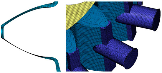
Figure 4.
Details of the mesh in the minimum volume and in the radial holes.
The fluid domain of the delivery pipe was generated directly in SimericsMP+ using the template mesh for cylinders, which allows obtaining a structured hexahedral grid. All other volumes were discretized with a general mesh generator that generated an unstructured Cartesian grid with cubic elements.
The different subdomains were connected to each other by means of the mismatched grid interface approach [34], which guaranteed to identify the overlapping areas between two neighbor regions; through these connections, a conservative treatment of mass, momentum and energy was applied, and the remaining nonoverlapping areas were considered as walls. The desired rotational speed was imposed at the driver gear (inner gear), while the driven gear speed was defined automatically by the software by means of the theoretical speed ratio, and the latter speed was also imposed at the rotating radial holes.
The static pressure was set as the boundary condition at the inlet port, while at the end of the delivery pipe, a Resistor Capacitor-orifice condition was imposed; this allowed introducing the flow–pressure relationship of the restrictor at the end of the pipe. If the instantaneous flowrate through the orifice (Qinst) and the environment pressure after the restrictor penv are known, the pressure at the boundary (pb), that is, upstream of the restrictor, is calculated as:
where Cd is the discharge coefficient; ρ is the fluid density, and d is the chosen diameter of the orifice. In this way, it was possible to have a variable pressure at the outlet, which is consistent with the instantaneous flow, instead of imposing a constant pressure value. Depending on the load condition to be simulated, the diameter of the orifice was changed in order to obtain the desired mean pressure in the pipe (according to experimental data).
The conjugate gradient squared linear solver was used for the velocity, and the algebraic multigrid solver was applied for the pressure, both applying first-order upwind numerical schemes. For the pressure–velocity coupling, the SIMPLE-S algorithm was employed.
Regarding the physical models, cavitation and aeration phenomena were simulated with the physical model “Equilibrium Dissolved Gas”, despite the fact that it had a negligible influence on the pressure at the pump delivery port. The turbulence model was not activated because it was demonstrated in previous studies that its effect does not influence the behavior of such machines [36].
A preliminary mesh sensitivity analysis was performed to determine the optimal mesh size. Configuration 3 with 4.5 bar of mean pressure and a pump speed of 1500 rpm was considered, and the pressure ripple in correspondence of pressure transducer S1 was used as the observed variable. The number of cells characterizing the rotor volume was changed in order to obtain total grid sizes between 845,000 and 2 million cells. It was found that a good convergence of residuals could be obtained with a grid of 1.5 million cells, which guaranteed a good approximation of the pressure waveform. However, it was found that such a result was still very sensitive to the time step chosen for the simulation. In fact, five values of the increment of the shaft angle were tested, between 1.5 degrees and 0.55 degrees. The delivery pressure in correspondence of the pressure transducer S1 is reported in Figure 5 both for the simulations and experimental values. The results show that a time step of 0.6 degrees is sufficient for obtaining a good approximation of the pressure waveform; thus, it was selected as the time step for all the simulations performed. Details about the final grid are reported in Table 2.
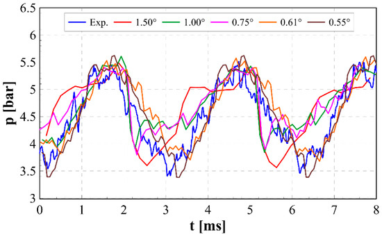
Figure 5.
Influence of the angular step on the delivery pressure.
Table 2.
Parameters of the mesh.
5. Validation
The developed model was validated by comparing the experimental pressure signals and mass flowrates with the corresponding numerical outcomes for different pump working conditions in terms of speed and load. The simulations were run on a workstation with an eight-core Intel® i7-9800X processor running at 3.8 GHz. About 30 h were needed to simulate a complete shaft revolution, and it typically took 2 revolutions to reach a steady-state point.
Figure 6, Figure 7 and Figure 8 show the comparison between the numerical and the experimental pressure signals. In particular, Configuration 3 in Figure 6 presents the comparison concerning the experimental pressure trace pup with the corresponding numerical trace (1200 rpm, load of 9.5 bar). In Figure 7, the pressure ripple validation in correspondence of the signal pdw is represented for Configuration 1 (1200 rpm, load of 4.2 bar). Finally, Figure 8 reports the pressure validation for the pdw signal with reference to Configuration 2 (1200 rpm, load of 6.5 bar). A schematic representation of the pump with the delivery line, which is reported in each figure, shows the approximate location at which the comparison has been performed. Owing to the different locations that were selected, a complete validation for pressure ripples along the entire delivery line was carried out. In fact, the numerical outcomes were generally in good agreement with the experimental signals close to the pump delivery port (Figure 6), to the middle of the pipe (Figure 7) and to the pipe extremity (Figure 8).

Figure 6.
Pressure validation close to the delivery port (1200 rpm, 9.5 bar).
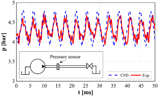
Figure 7.
Pressure validation close to the middle of the delivery line (1200 rpm, 4 bar).

Figure 8.
Pressure validation close to the pipe extremity (1200 rpm, 6.5 bar).
A further model validation was performed by comparing the numerical mass flowrate with the one measured by means of the flowmeter presented in Section 3, and the results are presented in Figure 9, Figure 10 and Figure 11, one for each configuration, at different working conditions. More precisely, Figure 9 refers to Configuration 1 (1200 rpm, load of 4 bar), Figure 10 to Configuration 2 (1200 rpm, load of 6.5 bar) and Figure 11 to Configuration 3 (1500 rpm, load of 9.5 bar). Because the flowmeter evaluates a flowrate averaged over the space, the numerical flowrate used for the comparison was taken in correspondence of the middle section between the pressure transducer location. It can be observed that the measured flowrate is in very good agreement with the numerical one in all the cases. In addition, in Figure 12, the comparison between the Fourier spectra obtained for the numerical flowrate and the measured one were reported for the working conditions shown in Figure 10 (in particular, the spectra were evaluated for the instantaneous flowrate minus its average value). As can be seen, the most relevant contribution occurs in correspondence of the ripple frequency for both the cases. Some small differences could be recognized in the experimental flowrate spectrum, and they could be ascribed to minor effects, such as the mechanical vibrations induced by the pump to the delivery line. The presented results, in addition to providing a further validation of the numerical model, prove that the three-dimensional effects close to the pump outlet do not introduce a pronounced distortion that leads to inaccurate flowrate measurements (that is based on the one-dimensional hypothesis, cf. Equations (1)–(4)). Indeed, the measured flowrates almost overlapped the numerical ones even in the proximity of the delivery port in the case of Configuration 1 (cf. Figure 9). Furthermore, when the flowmeter worked with Configuration 3 (the pressure sensors were installed at a distance L = 447 mm), the measured flowrate did not show any particular difference with respect to those obtained with the other flowmeter configurations. This becomes evident in Figure 13 with the comparison between the flowrates measured with the different flowmeter configurations for the same test case (1200 rpm, load of 4 bar). The differences that are present between the flowrate time histories in Figure 13 occur because such flowrates were acquired during tests with different installations. Therefore, the comparison is affected by a lack of perfect repeatability in the same working conditions after the reinstallation.

Figure 9.
Comparison between the numerical and the experimental flowrates (1200 rpm, 4 bar—Configuration 1).

Figure 10.
Comparison between the numerical and the experimental flowrates (1200 rpm, 6.5 bar—Configuration 2).
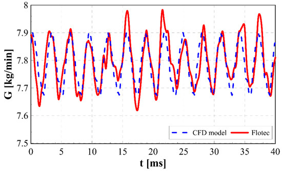
Figure 11.
Comparison between the numerical and the experimental flowrates (1500 rpm, 9.5 bar—Configuration 3).

Figure 12.
Comparison between the numerical and experimental flowrates Fourier spectra (1200 rpm, 6.5 bar, Configuration 2).

Figure 13.
Comparison between experimental flowrates measured with different flowmeter configurations for the same working condition (1200 rpm, 4 bar).
6. Application of the Numerical Model to Incomplete Filling Conditions
Simulations were performed with the validated 3D model of the pump by selecting high values of the pump speed, up to the condition of incomplete filling. Such a phenomenon occurs when the fluid does not have enough time for completely filling the rotating interteeth volumes during the suction phase. When the interteeth spaces connect to the delivery side, a sudden backflow originates; in this stage, the reversed flowrate is a function of the delivery pressure and of the current flow-area. Only when the interteeth spaces have been filled, is the flow direction abruptly inverted, and the flowrate is controlled by the time derivative of the variable volumes, which is a function of the geometric parameters of the gears. The reverse flow implies a significant increment of the flow ripple, due to a narrow and highly negative peak.
In order to understand the capability of the high-pressure flowmeter algorithm to measure the flowrate, even in this condition of a high flow ripple, a speed of 3500 rpm was imposed. The simulation had the aim of reproducing the incomplete filling in order to obtain a backflow for increasing the pump flow ripple. A quantitative evaluation of the amount of missing flowrate was out of the scope of the paper, because it would have required the simulation of the entire suction line. Hence, the presented simulated results must be considered as a qualitative example.
In Figure 14, the total gas mass fraction is shown on the midplane of the gears. On the pump inlet side, the increment of the volume between the two gears is not completely compensated by the flowrate entering the interteeth spaces through the radial holes. The oil is pushed outward by the centrifugal force and fills the chambers of the outer gear, while the interteeth volumes of the inner gear remain partially empty, once they have been isolated by the crescent.
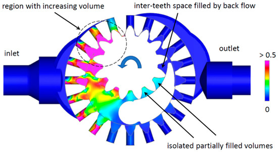
Figure 14.
Total gas volume fraction at 3500 rpm (0 only liquid phase, 1 only gas phase).
Different numerical pressure traces were used as input data to the flowmeter. In particular, the numerical pressure time history detected 14 mm from the delivery port was selected as the pup signal, while for the pdw signal, different distances with respect to pup (i.e., different L values in Equation (4)) were chosen, i.e., 100 mm, 200 mm and 400 mm.
When L is equal to 200 mm and to 400 mm, two layouts, such as those referring to Configuration 1 and Configuration 3, respectively, were selected, and the corresponding numerical pressure traces are reported in Figure 15. By applying Equation (4), three instantaneous flowrates were determined, one for each pdw trace; these flowrates were then compared with the numerical ones detected in the delivery pipe cross-section area located at half of the distance between the pressure signals. Figure 16 reports these comparisons, where the continuous lines refer to the flowrates obtained by means of Equation (4), while the numerical flowrates are represented with symbols (a scheme is reported in the upper left part of the figure and indicates the different cross-section areas, at which the numerical flowrates were detected). As can be inferred, when the distance L between the pressure traces is equal to 100 mm (line and symbols in magenta) and 200 mm (line and symbols in green), the flowmeter results are in very good agreement with the numerical model ones. On the other hand, when the two considered pressure signals are too far from each other, as in the case with L = 400 mm (line and symbols in red), the flowmeter is not capable of providing an accurate flowrate measurement. It was verified that, at this working condition, the numerical flowrate obtained by means of the 3D numerical model increases its amplitude travelling from the pump delivery to the pipe end. This is caused by a resonance effect on the pipe, since the flowrate ripple frequency value (obtained from the pump speed and the number of teeth of the internal gears) is close to the pipe’s natural frequency. The latter can be calculated by means of a simple 1D numerical model consisting of a pipe with the same geometrical features of the delivery line and a valve installed at the pipe end. When this valve is suddenly closed, stopping the liquid flow through the duct, some pressure waves are triggered and move back and forth with a certain frequency, which is the pipe’s natural one. When the flowrate ripple frequency approaches the natural frequency of the pipe, an excessive distance between the two pressure transducers leads to an inaccurate measure of the flowrate by means of Equation (4), due to the significant differences existing between the time histories of the space-averaged flowrate over distance L and the local flowrate at any point along the distance L.

Figure 15.
Simulated pressure traces as function of time for different pipe cross-section areas at 3500 rpm. The colors refer to the different cross sections indicated along the pipe.

Figure 16.
Comparison between the simulated flowrates (symbols) and the ones obtained based on Equation (4) algorithm (continuous line) at different pipe cross-section areas at 3500 rpm.
7. Conclusions
The flow ripple of an internal gear pump was measured by means of an innovative high-pressure instantaneous flowmeter (labeled as Flotec), installed on the pump delivery line. The flowmeter algorithm is based on the momentum balance and continuity equations written for a 1D unsteady flow. By combining them, an equation giving the instantaneous flowrate fluctuation with respect to the time-averaged value can be obtained as a function of the difference between two measured pressure signals, namely pup and pdown. The pressure transducers employed to measure pup and pdown were installed along the delivery line with three different configurations, where the distance between the sensors and between the delivery port was varied. Tests were performed for different working conditions in terms of the pump speed and load, the latter being modified by means of a variable diameter orifice installed at the delivery pipe’s extremity. For all the tested cases, the time-averaged pump-delivered flowrate was measured by means of a low-pressure Coriolis flowmeter.
A comprehensive 3D numerical model of the pump and its delivery line were developed in SimericMP+. The pump numerical model was validated successfully by comparing the numerical pressure traces, obtained at different locations along the delivery line, with the experimental ones and by comparing the numerical flowrate patterns with the ones measured by means of the Flotec. In particular, the different configurations of the flowmeter are all capable of correctly measuring the pump-delivered flowrate. A further validation was given by means of the comparison of the Fourier spectra of the numerical and the experimental flowrates. Simulations were then performed with the validated 3D model at high values of the pump speed, up to the condition of incomplete filling. The obtained numerical pressure traces were used as input data for the Flotec in order to verify its predictability under these severe conditions. If the distance between the pressure signals is lower than 200 mm, the flowrate obtained by the Flotec algorithm matches the one provided by the 3D numerical model. Instead, for distances higher than 200 mm, the flowrate measure accuracy reduces since the pump ripple frequency at these working conditions approaches the natural frequency of the pipe. Therefore, the flowrate shape changes significantly along the pipe, due to a resonance effect; this leads to a wrong prediction of the space-averaged instantaneous flowrate if the distance between the pressure sensors is too long.
Author Contributions
Conceptualization, A.F. and M.R.; methodology, O.V. and M.R.; software, P.F.; validation, P.F, O.V. and P.P; formal analysis, O.V.; data curation, O.V. and P.P.; writing—original draft preparation, M.R., O.V. and A.F.; writing—review and editing, M.R. and A.F.; supervision, M.R.; funding acquisition, A.F. All authors have read and agreed to the published version of the manuscript.
Funding
The research has received a financial support in the frame of a national call for “Proof of Concept” projects, promoted by Fondazione Compagnia di San Paolo, LINKS Foundation and LIFTT.
Institutional Review Board Statement
Not applicable.
Informed Consent Statement
Not applicable.
Data Availability Statement
Not applicable.
Acknowledgments
The authors thank Zhiru Jin for her contribution in the drawing of the 3D CAD model of the pump.
Conflicts of Interest
The authors declare no conflict of interest.
References
- Padovani, D.; Ketelsen, S.; Schmidt, L. Downsizing the electric motors of energy-efficient self-contained electro-hydraulic systems by using hybrid technologies. In Proceedings of the BATH/ASME 2020 Symposium on Fluid Power and Motion Control, Virtual, 9–11 September 2020. [Google Scholar] [CrossRef]
- Casoli, P.; Scolari, F.; Minav, T.; Rundo, M. Comparative energy analysis of a load sensing system and a zonal hydraulics for a 9-tonne excavator. Actuators 2020, 9, 39. [Google Scholar] [CrossRef]
- Casoli, P.; Zardin, B.; Ardizio, S.; Borghi, M.; Pintore, F.; Mesturini, D. The Hydraulic Power Generation and Transmission on Agricultural Tractors: Feasible architectures to reduce dissipation and fuel consumption-Part. E3S Web Conf. 2020, 197, 07010. [Google Scholar] [CrossRef]
- Qu, S.; Fassbender, D.; Vacca, A.; Busquets, E. A cost-effective electro-hydraulic actuator solution with open circuit architecture. Int. J. Fluid Power 2021, 22, 233–258. [Google Scholar] [CrossRef]
- Li, P.Y.; Siefert, J.; Bigelow, D. A hybrid hydraulic-electric architecture (HHEA) for high power off-road mobile machines. In Proceedings of the ASME/BATH 2019 Symposium on Fluid Power and Motion Control, Longboat Key, FL, USA, 7–9 October 2019. [Google Scholar] [CrossRef]
- Fresia, P.; Rundo, M.; Padovani, D.; Altare, G. Combined speed control and centralized power supply for hybrid energy-efficient mobile hydraulics. Autom. Constr. 2022, 140, 104337. [Google Scholar] [CrossRef]
- Harrison, A.M.; Edge, K.A. Reduction of axial piston pump pressure ripple. Proc. IMechE Part I J. Syst. Control Eng. 2000, 214, 53–63. [Google Scholar] [CrossRef]
- Marinaro, G.; Frosina, E.; Senatore, A. A numerical analysis of an innovative flow ripple reduction method for external gear pumps. Energies 2021, 14, 471. [Google Scholar] [CrossRef]
- Kim, T.; Ivantysynova, M. Active vibration / noise control of axial piston machine using swash plate control. In Proceedings of the ASME/BATH 2017 Symposium on Fluid Power and Motion Control, Sarasota, FL, USA, 16–19 October 2017. [Google Scholar] [CrossRef]
- Casoli, P.; Pastori, M.; Scolari, F.; Rundo, M. Active pressure ripple control in axial piston pumps through high-frequency swash plate oscillations—A theoretical analysis. Energies 2019, 12, 1377. [Google Scholar] [CrossRef]
- Hagstrom, N.; Harens, M.; Chatterjee, A.; Creswick, M. Piezoelectric actuation to reduce pump flow ripple. In Proceedings of the ASME/BATH 2019 Symposium on Fluid Power and Motion Control, Longboat Key, FL, USA, 7–9 October 2019. [Google Scholar] [CrossRef]
- Casoli, P.; Vescovini, C.M.; Scolari, F.; Rundo, M. Theoretical Analysis of Active Flow Ripple Control in Positive Displacement Pumps. Energies 2022, 15, 4703. [Google Scholar] [CrossRef]
- Shang, Y.; Tang, H.; Sun, H.; Guan, C.; Wu, S.; Xu, Y.; Jiao, Z. A novel hydraulic pulsation reduction component based on discharge and suction self-oscillation: Principle, design and experiment. Proc. IMechE Part I J. Syst. Control Eng. 2022, 234, 433–445. [Google Scholar] [CrossRef]
- Rundo, M. Theoretical flow rate in crescent pumps. Simul. Model. Pract. Theory 2017, 71, 1–14. [Google Scholar] [CrossRef]
- Johnston, D.N.; Drew, J.E. Measurement of positive displacement pump flow ripple and impedance. Proc. ImechE Part I J. Syst. Control Eng. 1996, 210, 65–74. [Google Scholar] [CrossRef]
- Weddfelt, K.G.; Pettersson, M.E.; Palmberg, J.O.S. Methods of reducing flow ripple from fluid power piston pumps—An experimental approach. SAE Trans. J. Commer. Veh. 1991, 100, 158–167. [Google Scholar] [CrossRef]
- Kojima, E.; Yu, J.; Ichiyanagi, T. Experimental determining and theoretical predicting of source flow ripple generated by fluid power piston pumps. SAE Trans. J. Commer. Veh. 2000, 109, 348–357. [Google Scholar] [CrossRef]
- Sanchugov, V.; Rekadze, P. New Method to Determine the Dynamic Fluid Flow Rate at the Gear Pump Outlet. Energies 2022, 15, 3451. [Google Scholar] [CrossRef]
- Edge, K.A.; Johnston, D.N. The ‘Secondary Source’ Method for the Measurement of Pump Pressure Ripple Characteristics Part 1: Description of Method. Proc. Inst. Mech. Eng. Part A J. Power Energy 1990, 204, 33–40. [Google Scholar] [CrossRef]
- Yu, J. Determining source fluidborne noise characteristics of automotive fluid power pumps. SAE Trans. J. Passeng. Car 2001, 110, 2087–2096. [Google Scholar] [CrossRef]
- Bramley, C.; Johnston, N. Comparison of methods for measuring pump flow ripple and impedance. In Proceedings of the ASME/BATH 2017 Symposium on Fluid Power and Motion Control, Sarasota, FL, USA, 16–19 October 2017. [Google Scholar] [CrossRef]
- Catania, A.E.; Ferrari, A. Development and assessment of a new operating principle for the measurement of unsteady flow rates in high pressure pipelines. Flow Meas. Instrum. 2009, 20, 230–240. [Google Scholar] [CrossRef]
- Ferrari, A.; Novara, C.; Paolucci, E.; Vento, O.; Violante, M.; Zhang, T. Design and rapid prototyping of a closed-loop control strategy of the injected mass for the reduction of CO2, combustion noise and pollutant emissions in diesel engines. Appl. Energy 2018, 232, 358–367. [Google Scholar] [CrossRef]
- Ferrari, A.; Novara, C.; Vento, O.; Violante, M.; Zhang, T. A new closed-loop control of the injected mass for a full exploitation of digital and continuous injection-rate shaping. Energy Convers. Manag. 2018, 177, 629–639. [Google Scholar] [CrossRef]
- Ferrari, A.; Pizzo, P.; Rundo, M. Modelling and experimental studies on a proportional valve using an innovative dynamic flow-rate measurement in fluid power systems. Proc. ImechE Part C J. Mech. Eng. Sci. 2018, 232, 2404–2418. [Google Scholar] [CrossRef]
- Corvaglia, A.; Ferrari, A.; Rundo, M.; Vento, O. Three-dimensional model of an external gear pump with an experimental evaluation of the flow ripple. Proc. ImechE Part C J. Mech. Eng. Sci. 2021, 235, 1097–1105. [Google Scholar] [CrossRef]
- Ferrari, A.; Vento, O. Influence of Frequency-Dependent Friction Modeling on the Simulation of Transient Flows in High-Pressure Flow Pipelines. ASME J. Fluids Eng. 2020, 142, 081205. [Google Scholar] [CrossRef]
- Batchelor, G.K. An Introduction to Fluid Dynamics; Cambridge University Press: Cambridge, UK, 2000. [Google Scholar] [CrossRef]
- Ferrari, A.; Pizzo, P. Optimization of an Algorithm for the Measurement of Unsteady Flow-Rates in High-Pressure Pipelines and Application of a Newly Designed Flowmeter to Volumetric Pump Analysis. ASME J. Eng. Gas Turbines Power 2016, 138, 031604. [Google Scholar] [CrossRef]
- Rundo, M.; Corvaglia, A. Lumped parameters model of a crescent pump. Energies 2016, 9, 876. [Google Scholar] [CrossRef]
- Pan, D.; Vacca, A. A numerical method for the analysis of the theoretical flow in crescent-type internal gear machines with involute tooth profile. In Proceedings of the ASME/BATH 2019 Symposium on Fluid Power and Motion Control, Longboat Key, FL, USA, 7–9 October 2019. [Google Scholar] [CrossRef]
- Du, R.; Chen, Y.; Zhou, H. Investigation into the lubricating gap between the ring gear and the case in internal gear pumps. Ind. Lubr. Tribol. 2018, 70, 454–462. [Google Scholar] [CrossRef]
- Ansari, B.; Aligholami, M.; Rostamzadeh Khosroshahi, A. An experimental and numerical investigation into using hydropower plant on oil transmission lines. Energy Sci. Eng. 2022, 1–14. [Google Scholar] [CrossRef]
- Ding, H.; Visser, F.C.; Jiang, Y.; Furmanczyk, M. Demonstration and validation of a 3D CFD simulation tool predicting pump performance and cavitation for industrial applications. J. Fluids Eng. 2011, 133, 011101. [Google Scholar] [CrossRef]
- Jiang, Y.; Furmanczyk, M.; Lowry, S.; Zhang, D.; Perng, C.Y. A Three-Dimensional Design Tool for Crescent Oil Pumps; SAE Technical Paper 2008-01-0003; SAE: Warrendale, PA, USA, 2008. [Google Scholar] [CrossRef]
- Rundo, M.; Altare, G. Lumped Parameter and Three- Dimensional Computational Fluid Dynamics Simulation of a Variable Displacement Vane Pump for Engine Lubrication. J. Fluids Eng. 2018, 140, 061101. [Google Scholar] [CrossRef]


Publisher’s Note: MDPI stays neutral with regard to jurisdictional claims in published maps and institutional affiliations. |
© 2022 by the authors. Licensee MDPI, Basel, Switzerland. This article is an open access article distributed under the terms and conditions of the Creative Commons Attribution (CC BY) license (https://creativecommons.org/licenses/by/4.0/).