2.1. Maintenance of Electrical Systems in Hospitals
Maintenance of power supply systems is particularly essential for safety and reliability in hospitals [
3] due to the consequences of failure. The complexity of today’s systems augments the need for proper maintenance. Although they were speaking about manufacturing, Ni et al. made a relevant point: “Maintenance operations in a modern manufacturing system are complex because they need the integration of several sources of information, including: (a) current machine conditions and its degradation profiles; (b) system configurations; (c) availability of maintenance crews and resources; (d) the current Work-In-Process (WIP) in the system; and (e) the throughput target” [
4]. According to Hennequin et al. (2016), preventive maintenance increases availability improves product quality, reduces costs, and generally improves productivity [
5]. Macchi et al. (2020) argue that “smart maintenance appears to be a promising concept to shape advanced maintenance systems built in the digital era” [
6]. At this point, there are many different preventive maintenance options, each with its benefits. The trick is to pick the best one. The optimal preventive maintenance will significantly improve efficiency [
7]. To this end, Lagrange et al. suggested that “the benefits provided by an improvement of the energy resilience… could achieve by installing a microgrid in a hospital fed by renewable energy sources” [
8]. Balali and Valipour (2021) proposed reducing energy consumption in hospitals and health centers using passive strategies when designing them. Unfortunately, very few studies have examined the use of this type of strategy in hospitals and health centers [
9]. In this way, some recent work has used modeling to discover better methods of hospital maintenance. For example, Yousefli et al. used hospital maintenance data for multi-agent simulation to improve workflow management. They found simulation reduced the time to respond to maintenance requests, an essential factor when dealing with critical systems [
10]. Christiansen tested a model approach using over 33,500 h of measurements from a German medical center to assess time-dependency and the weekly sum of the demand for electrical energy due to medical laboratory plug loads [
11]. Maintaining a hospital’s electricity system is essentially a risk management task; operators must always be vigilant, trained in safety measures, and understand and use the latest technology. RAMS aims to prevent failures, breakdowns, and delays in production and service processes to improve time, cost, and system performance. Despite the ubiquity of the RAMS concept, more research is needed on hospital assets to ensure quality management efforts for internal and external customer satisfaction, guided by international standards. RAM analysis is the basis for complex system performance analysis [
12]. Sutton (2015) add that RAM programs are “an integral part of any risk management system” [
13]. Sharma and Sharma (2012) pointed out that the popularity of RAM has increased substantially in recent years due to rising operation and maintenance costs [
14]. Pirbhulal et al. present RAMS analysis of critical infrastructures (CIs) subject to failure modes [
15]. Reliability, Availability, Maintenance, and Safety are essential to pay attention to; these variables ensure that products and services are not interrupted and sustainable. Therefore, an experienced manager must always be aware of risk management in the hospital context.
2.2. Petri Nets
This paper is closely related to the evolution of the authors’ research. The following few sections are strongly supported by previous work [
1]. A Petri net (PN) can be defined as follows:
The Petri net consists of 5 tuples N = (P, T, I, O, Mo), which is defined as the five tuples N = (P, T, 1, 0, Mo) by the Petri net, where:
P = {P1, P2, …, Pm} is a finite set;
T = {t1, t2, …, tn} is a finite transition set, P U T and PT =;
I(P, T) → N is an input function that defines an arc directed from a place to a transition, where N is the set of negative integers;
(T, P) → N is the output function that defines the arc from the transition to the place, and Mo: P → N is the starting point.
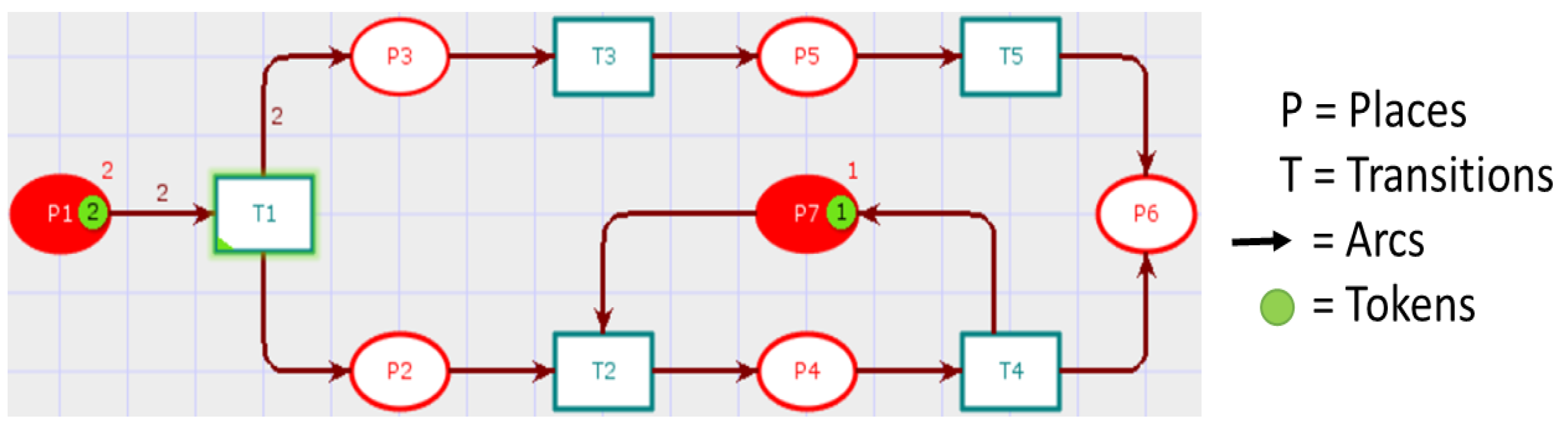
The marking (M) is the movement of tokens to places in the Petri net system. The number and position of tokens may change during implementation due to the Petri network’s transitions. A simulation example shown in
Figure 1. The Petri net contains:
P = {p1, p2, …, p7};
T = {t1, t2, …, t5};
I (t1, p1) = 2, I (t1, pi) = 0 for i = 2, 3, …, 7;
I (t2, p2) = 1, I (t2, p7) = 1, I (t2, pi) = 0 for i = 1, 3, 4, 5, 6;
O (t1, p2) = 1, O (t1, p3) = 2, O (t1, pi) = 0 for i = 1, 4, 5, 6, 7;
O (t2, p4) = 1, O (t2, pi) = 0 for i = 1, 2, 3, 5, 6, 7;
Mo = (2 0 0 0 0 0 1)T.
Petri nets are widely used for modeling asynchronous events, processing synchronization, concurrent operations, sequential operations, conflicts, or resource sharing [
16]. Pinto et al. conclude the importance of Petri nets in maintenance management because it is beneficial for analyzing and simulating complex systems to increase asset function and operation reliability and availability [
1]. Grunt and Briš suggest using an extension of Petri nets, i.e., Stochastic Petri Nets (SPNs), as a suitable modeling tool for time-dependent events such as fire escalation or gas cloud explosion [
17]. Aloini et al. used Colored Petri Nets (CPNs) to model risk factors in Enterprise Resource Planning (ERP) projects to deal with the problem of interdependence in risk assessment [
18]. Meanwhile, Li et al. proposed a layered Petri net method to describe coupling relations and add flexibility to computational processes during complex rule-based risk analysis and assessment [
19]. In another work, Li et al. propose a Timed Colored Petri net (TCCP-net) and a time–space coupling safety constraint to conduct a time–space coupling hazard analysis [
20]. Liu et al. also defined a probabilistic Colored Petri Net model comprising basic models, rules, logical operators, and transitions that describe threat propagation between nodes [
21].
2.4. Stochastic Time Petri Nets (STPNs) and Markov Chains
Stochastic time Petri nets (STPNs) combine stochastic processes with Petri net theory and are used to find answers to complicated and challenging problems. We use STPNs to model and simulate the behavior of a system to identify potential problems. This approach is essential when a system does not have historical data, but the organization needs rigorous knowledge on its reliability, availability, and maintainability to improve its performance. In their work on risk assessment of groundwater contamination, Jiang et al. created the fuzzy stochastic model that combines the input vector fuzzy cluster with the activation function of the radial basis in a stochastic neural network [
30]. Finally, Sharifi et al. used a stochastic fuzzy-robust approach to tackle the uncertainty of second-generation biofuel network design parameters. They applied the weighted sum method [
31]. In their study of the reliability of a system dedicated to renewable energies using stochastic Petri nets, Mahdi et al. initiated a “time factor”, whereby the associated times on each transition were random variables following distribution laws. They also proposed using Monte Carlo simulations, Markovian chains, or other state diagrams [
32]. On the other hand, Volovoi and Peterson (2011) distinguish between Markov chains and SPN, noting that each state represents the system as a whole in the former. Still, the states of individual components are described in the latter, and the systems state is inferred from its components [
33]. Finally, Dhople et al. developed a stochastic hybrid systems framework. It is usually used in system performance analysis to analyze the Markov model. This framework is based on an analytical tool developed for stochastic processes called stochastic hybrid systems [
34]. Wang et al. incorporated the Markov chain concept into a fuzzy stochastic prediction of stock indexes to attain better accuracy and confidence [
35]. To sum up, as these examples suggest, the STPN is a sophisticated tool that can be used to understand complex and multidimensional systems.
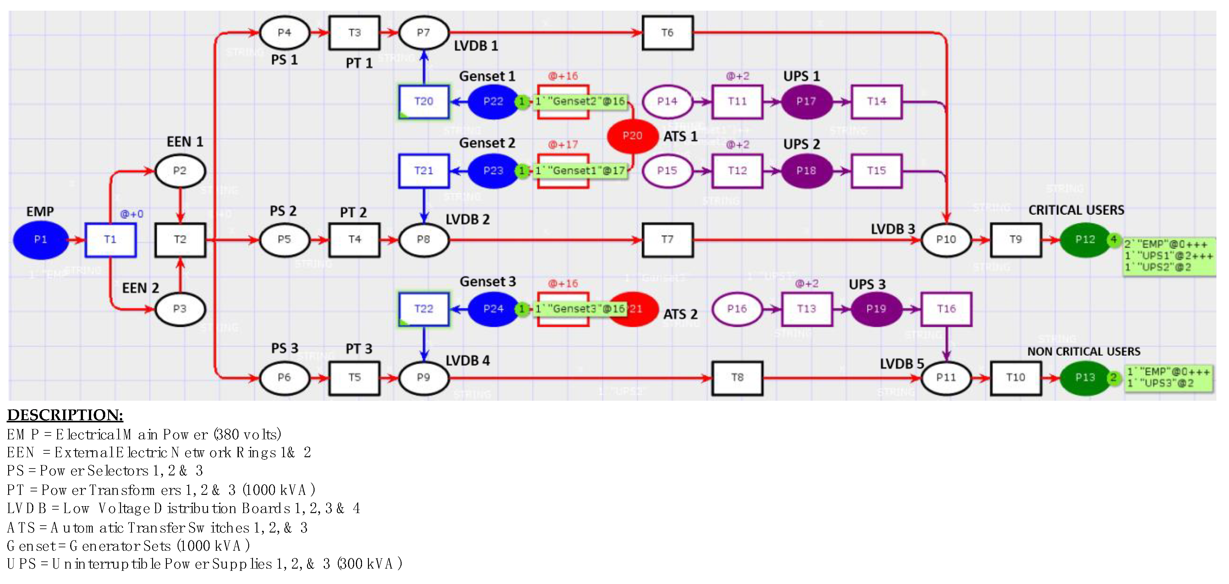
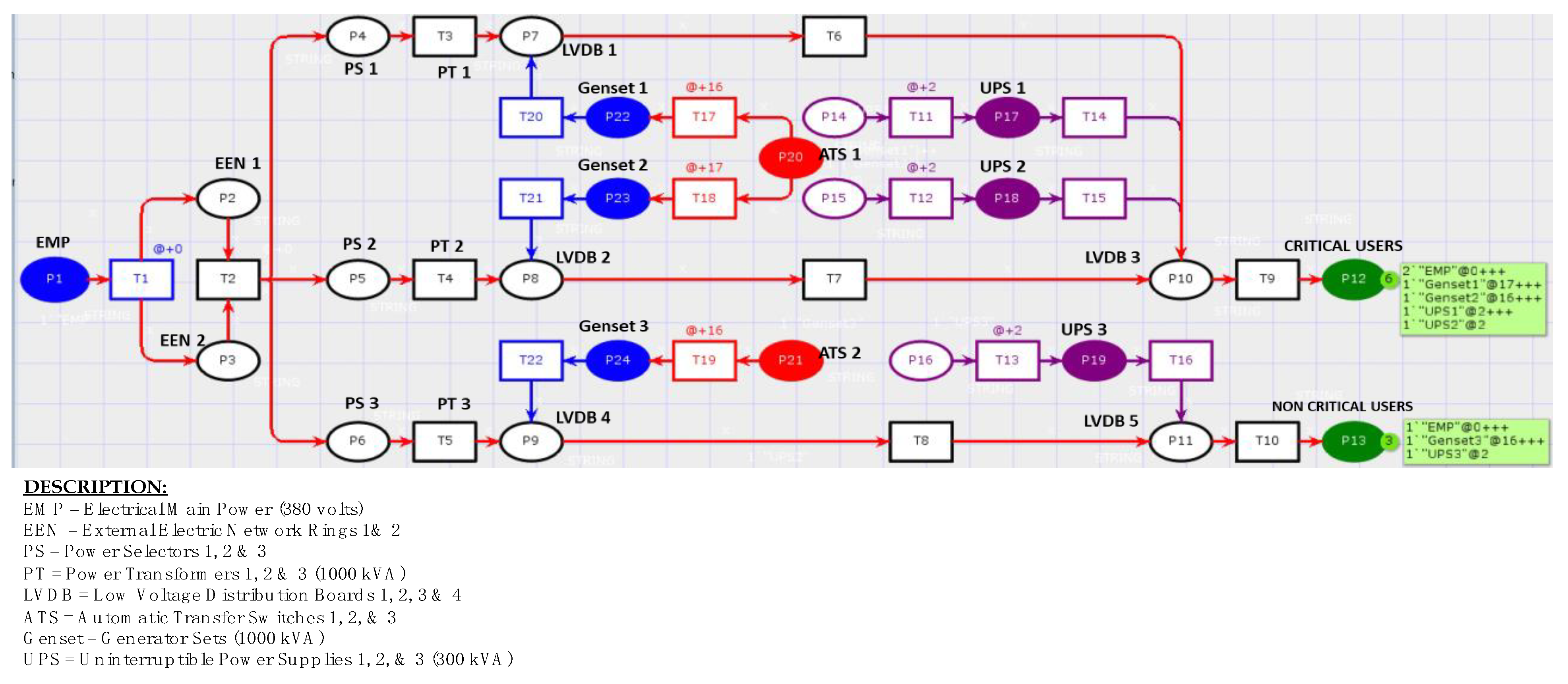
The Stochastic Petri Net (SPN) is a six-tuple (P, T, I, O, M0, ) where (P, T, I, O, M0) is the Petri net, : TR is the set of levels where k is the exponential distribution rate of the individual ignition time Gk (x|M) is related to the transition tk, and
P (Places) = {P1, P2, …, P24};
T (Transitions) = {T1, T2, …, T22};
I (Input);
O (Output);
M0 (Marking).
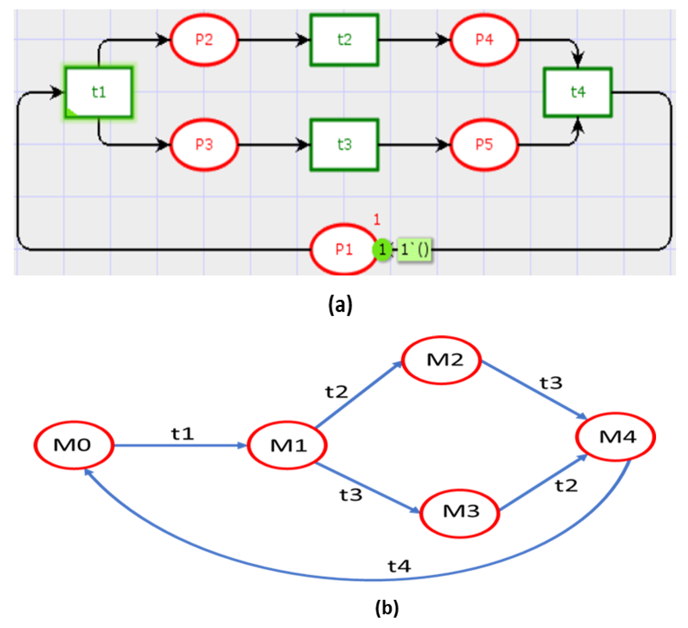
With: M0 = (1 0 0 0 0) T, M1 = (0 1 1 0 0)T, M2 = (0 0 1 1 0)T, M3 = (0 1 0 0 1)T, and M4 = (0 0 0 1 1)
T.
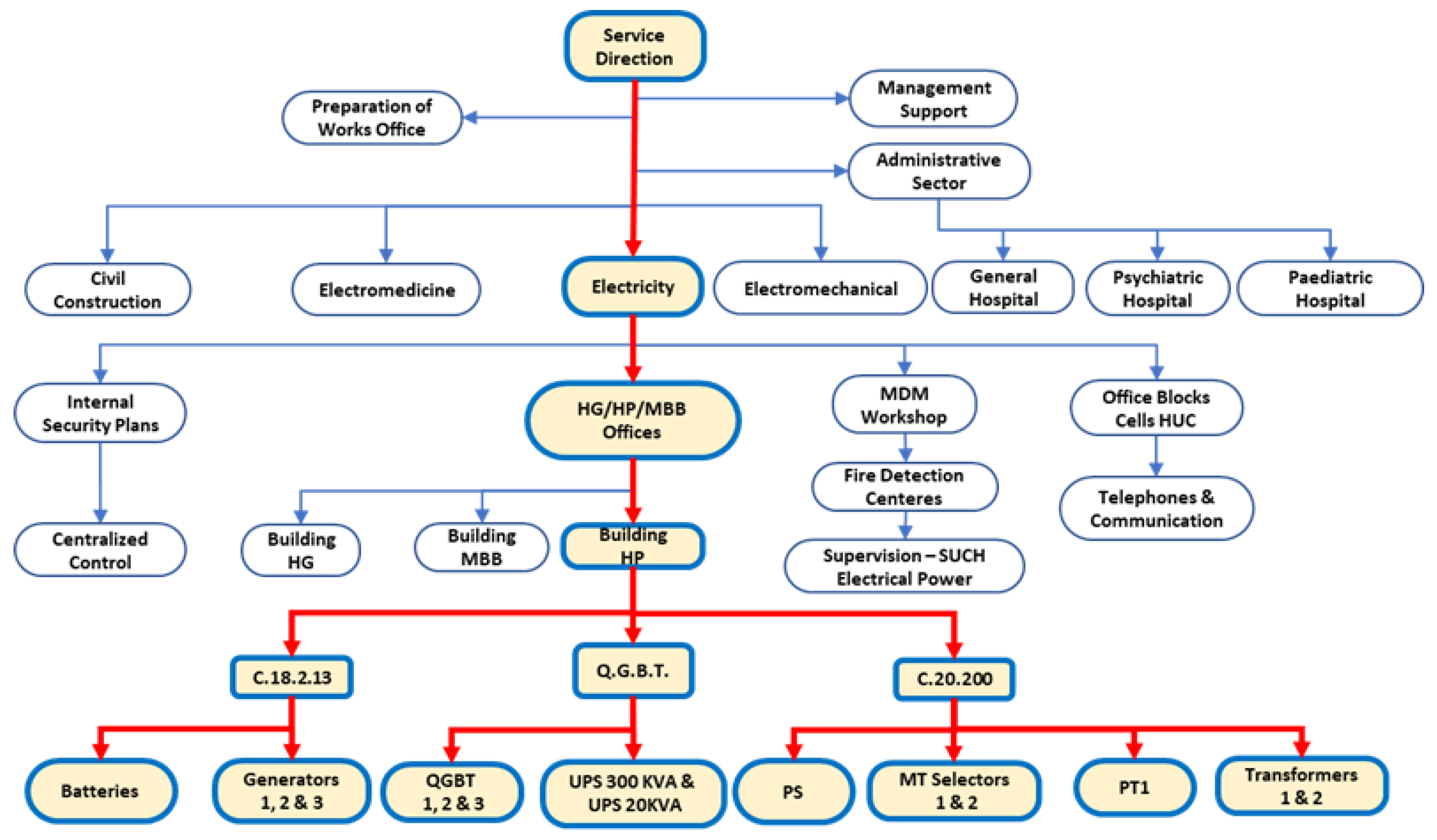
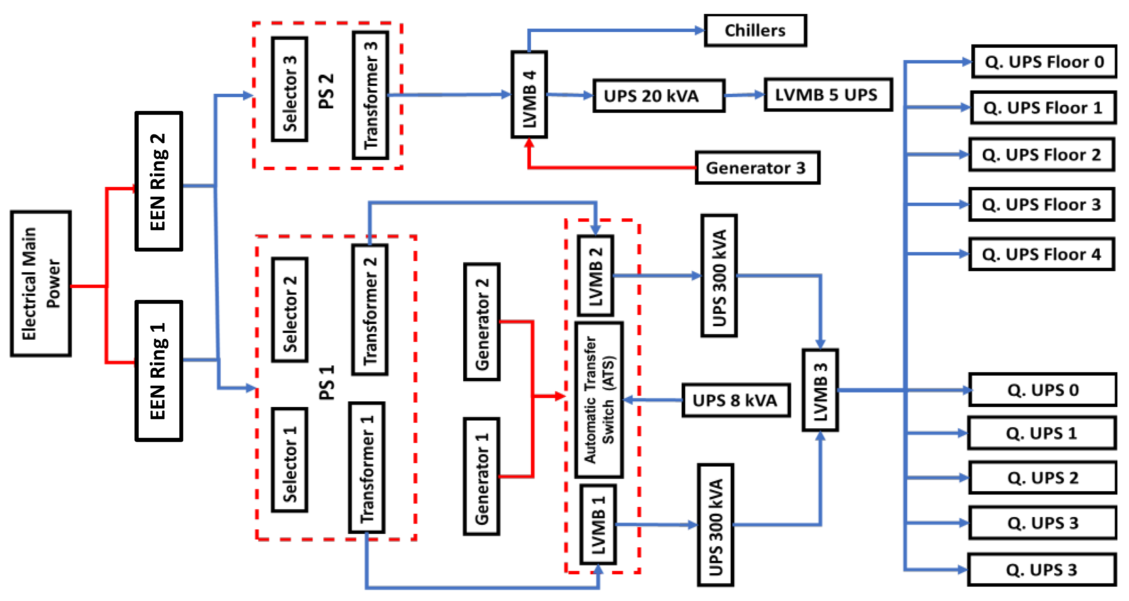
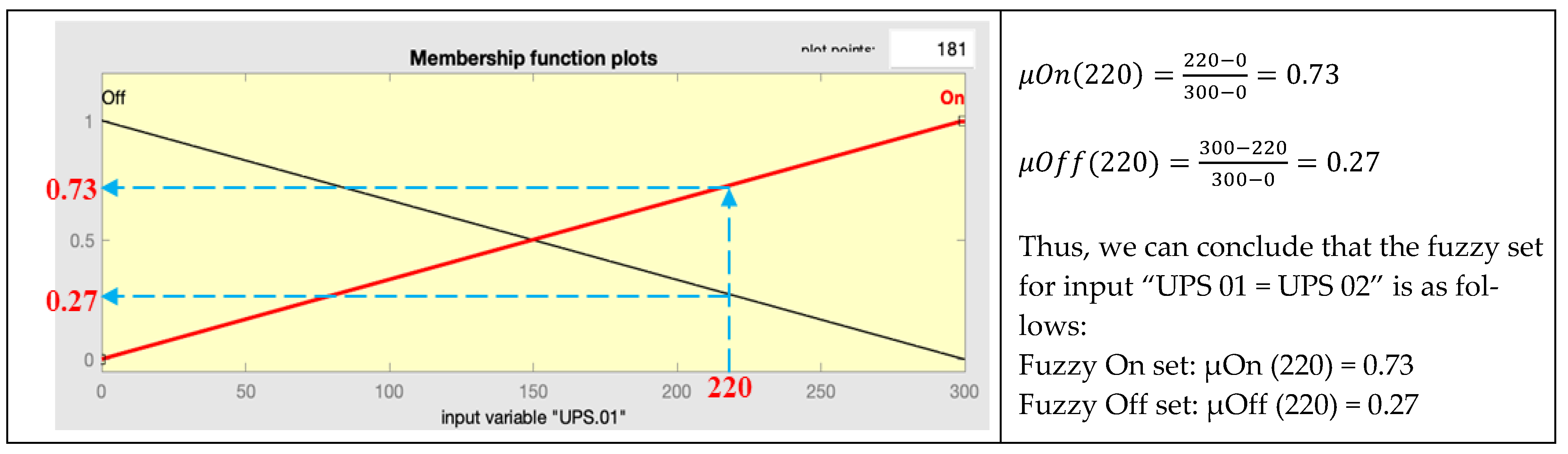
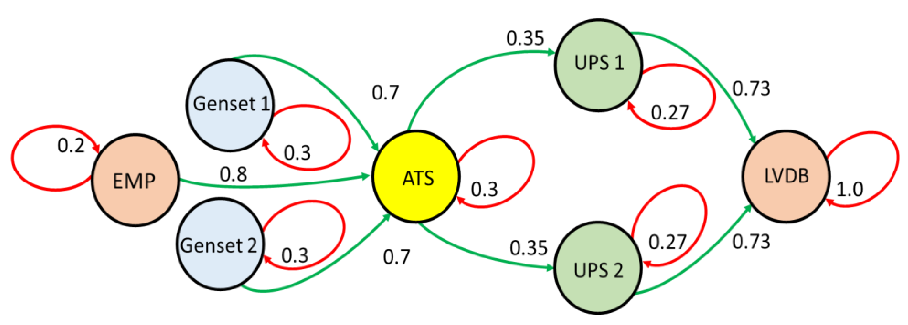
Our case study is a large hospital in Europe without historical data. In earlier work, we used Petri nets to identify the most critical equipment and systems on the electrical power supply system. To determine the reliability function, we used FIS [
2]. We use another approach to compare them in this work and confirm the results: the “Stochastic versus Fuzzy” approach. We also use Markov chains for simulation and to simplify the matrix. The supporting concepts are as follows:
Stochastic Classification Process
1. A stochastic process is a time-dependent random variable. Therefore, we have a function with two arguments, X (t, ω), where:
t∈ is time, with as a possible set of times, usually (0, ∞), (−∞, ∞),
{0, 1, 2,…}, or {…−2, −1, 0, 1, 2,…};
ω∈ Ω, as before, is the experimental result, where is the entire sample space.
The value of X (t, ω) is called the state.
2. A stochastic process X (t, ω) is a discrete state if the variable Xt (ω) is discrete for each time t, and a continuous state if Xt (ω) is also continuous.
3. The stochastic process X (t, ω) is a discrete-time process if the specified time consists of separate and isolated points. It is a continuous-time process if it is a connected interval; note that it can be infinite.
4. A stochastic process X(t) is a Markov chain if for all t1 < ... < tn < t, and there is a set A; A1,…, An
P (X (t) ∈ A | X (t1) ∈ A1,…, X (tn) ∈ An}
= P (X (t) ∈ A | X (tn) ∈ An).
The conditional distribution of X(t) is the same in two different conditions:
The continuous-time Markov chain is a stochastic process with a Markov property. The distribution of future conditions at time t + s, given the present state, if all past states depend only on the current state and do not depend on the past is as follows:
P {future | past, present} = P {future | now}.
Then, only its current state matters for the future development of the Markov process, and it does not matter how the process came to be in this state.
Discrete-Value Process and Continuous-Value. X (t) is a discrete-value process if the set of all possible values of X (t) at all times t is the computable set Sx; otherwise, X (t) is a continuous value process.
Discrete-time and continuous-time processes. An educational process X(t) is a discrete-time process if X(t) is defined only for a set of instantaneous times, tn = nT, where T is a constant and n is an integer; otherwise, X(t) is a continuous-time process.
A Markov chain with discrete-time (discrete-time Markov chain) is a process with discrete-time when X(t) has a discrete value. Mathematically, the probability of moving from state i to j in time t is expressed as:
pij (t) = P (X (t + 1) = j | X (t) = i)
= P (X (t + 1) = j | X (t) = i, X (t − 1) = h, X (t − 2) = g,…)
The probability of transition to the h-step is expressed as:
Pij (h) (t) = P (X (t + h) = j | X (t) = i)
The three main procedures involved in the Markov analysis process are as follows:
Construct a transition probability matrix;
Calculate the probability of an event in the future;
Determine the steady-state conditions.
Matrix Approach: The transition probabilities of a step
pij can be written in an n × n transition probability matrix:
The intersection of row
i-th and column
j-th intersection is
pij, the probability of transition from state
i to state
j. From every state, a Markov chains make transitions to one and only one state. States destinations are disjoint and exhaustive events; therefore, the total of each row is equal to 1:


