Stacked LSTM Sequence-to-Sequence Autoencoder with Feature Selection for Daily Solar Radiation Prediction: A Review and New Modeling Results

Abstract

We review the latest modeling techniques and propose new hybrid SAELSTM framework based on Deep Learning (DL) to construct prediction intervals for daily Global Solar Radiation (GSR) using the Manta Ray Foraging Optimization (MRFO) feature selection to select model parameters. Features are employed as potential inputs for Long Short-Term Memory and a seq2seq SAELSTM autoencoder Deep Learning (DL) system in the final GSR prediction. Six solar energy farms in Queensland, Australia are considered to evaluate the method with predictors from Global Climate Models and ground-based observation. Comparisons are carried out among DL models (i.e., Deep Neural Network) and conventional Machine Learning algorithms (i.e., Gradient Boosting Regression, Random Forest Regression, Extremely Randomized Trees, and Adaptive Boosting Regression). The hyperparameters are deduced with grid search, and simulations demonstrate that the DL hybrid SAELSTM model is accurate compared with the other models as well as the persistence methods. The SAELSTM model obtains quality solar energy prediction intervals with high coverage probability and low interval errors. The review and new modelling results utilising an autoencoder deep learning method show that our approach is acceptable to predict solar radiation, and therefore is useful in solar energy monitoring systems to capture the stochastic variations in solar power generation due to cloud cover, aerosols, ozone changes, and other atmospheric attenuation factors.

1. Background Review

Demand for cleaner, green energy has been rapidly increasing in last few years as a result of the negative impacts of fossil fuel-based energies to our environment and their contributions to climate change. This has produced a growing interest on clear energy resources such as solar and wind power [1]. According to a report released by the International Renewable Energy Agency (IRENA), despite the COVID-19 pandemic, more than 260 GW of renewable energy capacity have been added in 2020, and this exceeds the previous record by nearly 50% [2]. One of the current most promising sources of energy is solar energy [3], particularly in photovoltaics (PV) technology, whose worldwide capacity (year 2020) has reached about the same level as the wind capacity, mostly because of expansions in Asia (78 GW), with significant capacity increases in China (49 GW) and Vietnam (11 GW). In addition, Japan added more than 5 GW, and on the other hand, the Republic of Korea added nearly 4 GW and the United States added 15 GW [2]. Moreover, the power output of PV panels is strongly correlated with Global Solar Radiation (GSR), which is influenced by many factors (for example, latitude, season, and sky conditions, among others) [4]. The GSR is highly intermittent and chaotic, and even the slightest fluctuation in solar radiation can have an impact on power supply security [5]. Considering this, the development of accurate GSR prediction models, especially those that can capture cloud cover effects on solar energy generation forecasts, is essential for ensuring an optimum energy dispatch and management practice. This becomes particularly important as rooftop solar power generation and its penetration into the grid increases.

There are usually four main types of models used in GSR prediction problems, which are classified into physical, empirical, statistical prediction, and Machine Learning (ML)-based models. The physical models look for relationships between GSR and other meteorological parameters [3], usually by means of Numerical Weather Prediction (NWP) systems. Despite its strong physical basis, there are challenges such as sourcing and selecting the inputs for NWP models [6,7,8], and there are also issues related to the high computation cost of these models. Among the most common models used is the empirical model, which is intended to develop a linear or nonlinear regression equation [9]. Although empirical models are easy and simple to operate, their accuracy is usually limited. Statistical models, such as the Autoregressive Integrated Moving-Average model (ARIMA) [10] and the Coupled Autoregressive and Dynamical System (CARDS) [11] model rely on the statistical correlation [12]. Although the precision of these statistical models is usually higher than empirical models, however, they fail to capture complex nonlinear relationships accurately between the GSR and other parameters. Furthermore, in statistical modeling process, historical data are taken into account, while other relevant weather conditions that influence solar GSR cannot be included [13]. ML-based approaches can be used to overcome this shortcoming by integrating various types of input data into prediction models, and these models have the ability to extract complex nonlinear features from multiple inputs [14]. During the last three decades, a wide range of ML models have been used for GSR prediction, such as Artificial Neural Networks (ANNs) [15,16], Recurrent Neural Networks (RNN) [14], evolutionary neural approaches [17,18], Extreme Learning Machines (ELM) [19,20,21,22], Ensemble Learning (EL) [23], Multivariate Adaptive Regression Spline (MARS) [24], Gaussian Processes [25], and Support Vector Machines (SVMs) [26,27,28], among others. These ML models offer higher accuracy than empirical and statistical models [29] as well as competitive behavior with less computational burden than NWP models, making them one of the most popular models that have been used previously in short-term [30], medium-term [31], and long-term [32] GSR prediction.

Despite having gained extensive attention in the past for several prediction applications, the ML-based approaches such as neural networks, ELMs, SVRs, etc., also suffer from a few major drawbacks: (a) selecting the correct input features for a model requires high expertise, thus making them unreliable and less capable of extracting the nonlinear features from GSR data [33]; (b) because of less generalization capability, these models are less effective in learning complex patterns and have the drawbacks of over-fitting, gradient disappearance, and excessive network training [34]; and (c) these models perform very well on relatively small datasets, but when the data size is huge, they may be subjected to instabilities and a rather slow convergence of their parameters [35]. Due to the tedious selection of features, a degree of over-fitting and somewhat high complexity linked to the datasets, exploring different promising approaches that relies on Deep Learning (DL) [36] to predict GSR is becoming the norm.

Models based on DL are proving useful in a multitude of areas for several reasons, including their ability to extract features faster, their power to generalize, and their capacity to handle big data [37]. The largest difference between conventional ML models and DL models is the number of transformations that the input data undergo before it reaches the output. In DL models, input data are transformed multiple times before the output is produced, whereas conventional ML models transform it only once or twice [38]. Consequently, DL models can learn highly complex patterns from data without any manual intervention and work extremely well for several applications such as image processing, pattern extraction, classification, and prediction. For instance, Long Short-Term Memory (LSTMs) networks are trending in solving time-series prediction problems, and thus, many studies have employed these models for GSR prediction [39,40,41,42,43,44]. Srivastava and Lessmann [45] developed an LSTM model using different meteorological parameters such as inputs based on air pressure, cloud cover, etc.; LSTM outperforms the Feed Forward Neural Networks (FFNN) and Gradient Boosting Regression (GBR) model for daily GSR prediction.

Aslam et al. [46] analyzed various state-of-the-art DL (LSTM, Gated Recurrent Unit (GRU)) and conventional ML (RNN, SVR, FFNN) models to predict GSR. Simulation results show that DL models perform better than the conventional ML models. Brahma and Wadhvani [47] proposed two different LSTM algorithms, namely Bidirectional LSTM (BiLSTM), Attention LSTM, and GRU for the prediction of daily GSR, and the results obtained suggest that BiLSTM has shown higher accuracy than other DL models. Furthermore, to improve the accuracy of GSR prediction, multiple ML or DL models were combined to take advantage of each single prediction model. The attention-based CNN model has been investigated by [48] in a study on the anomaly detection in quasi-periodic time series based on automatic data segmentation, while the study of [49] developed a data-driven evolutionary algorithm with perturbation-based ensemble surrogate method. Bendali et al. [50] propose an innovative hybrid method utilizing a genetic algorithm (GA) to optimize a deep neural network for solar radiation forecasting (GRU, LSTM, and RNN). Zang et al. [13] and Ghimire et al. [51] proposed a deep hybrid model that combines Convolutional Neural Network (CNN) and LSTM for GSR prediction. Likewise, Husein and Chung [52] proposed a hybrid, called LSTM-RNN, for daily GSR prediction. For a study in Queensland, Australia, Deo et al. [53] and Ghimire et al. [54] investigated the use of wavelet transform methods to improve solar radiation predictions, showing the efficacy of input data decomposition on the improved performance of wavelet-based models.

In accordance with this review, the following aspects summarize many of the shortcomings of existing studies: (a) many studies used historical records or antecedent values of GSR to predict the future thereby, ignoring the meteorological factors as inputs; (b) in the modeling process of these hybrid models, no feature selection algorithm has been used; (c) model testing results were unable to measure uncertainties in GSR prediction; and (d) nevertheless, not many studies have focused on the persistence model, which is difficult to surpass [55], sometimes even by the most advanced models [56].

Therefore, a key objective of this study is to address the research gaps listed above and develop a new DL hybrid Stacked LSTM Sequence to Sequence Autoencoder method, denoted as the SAELSTM model, adopted for daily GSR prediction at six solar farms in Queensland, Australia. The major contributions in developing the DL hybrid stacked LSTM sequence to sequence autoencoder (i.e., SAELSTM) model can be summarized as follows: (a) predictors from global climate model (GCM) meteorological data and ground-based data from Scientific Information for Landowners (SILO) were used for GSR predictions; (b) a Manta Ray Foraging Optimization (MRFO)-based feature selection process was implemented to select the best set of features for the problem; (c) LSTM-based seq2seq architectures were explored for GSR prediction and compared with Deep Neural Network (DNN), Gradient Boosting Regression (GBM), Random Forest Regression (RFR), Extremely Randomized Trees (ETR), and Adaptive Boosting Regression (ADBR), and (d) a prediction interval (PI) was calculated via quantile regression to quantify the level of uncertainty in the daily GSR prediction.

The structure of the paper is as follows: next, we summarize the most important characteristics of the main algorithms used in the proposed hybrid DL approach of GSR prediction, including the MRFO algorithm, LSTM network, the SAELSTM approach, and a summary of DL methods for comparison. Section 3 describes the study area considered and the data available for this study. Section 4 describes the proposed predictive model development for GSR prediction problems, and Section 5 discusses the results obtained and describes the comparison with alternative methods. Finally, Section 6 closes the paper with some conclusions and remarks on the research carried out and the results obtained.

2. Review of Theoretical Framework for ML and DL Techniques

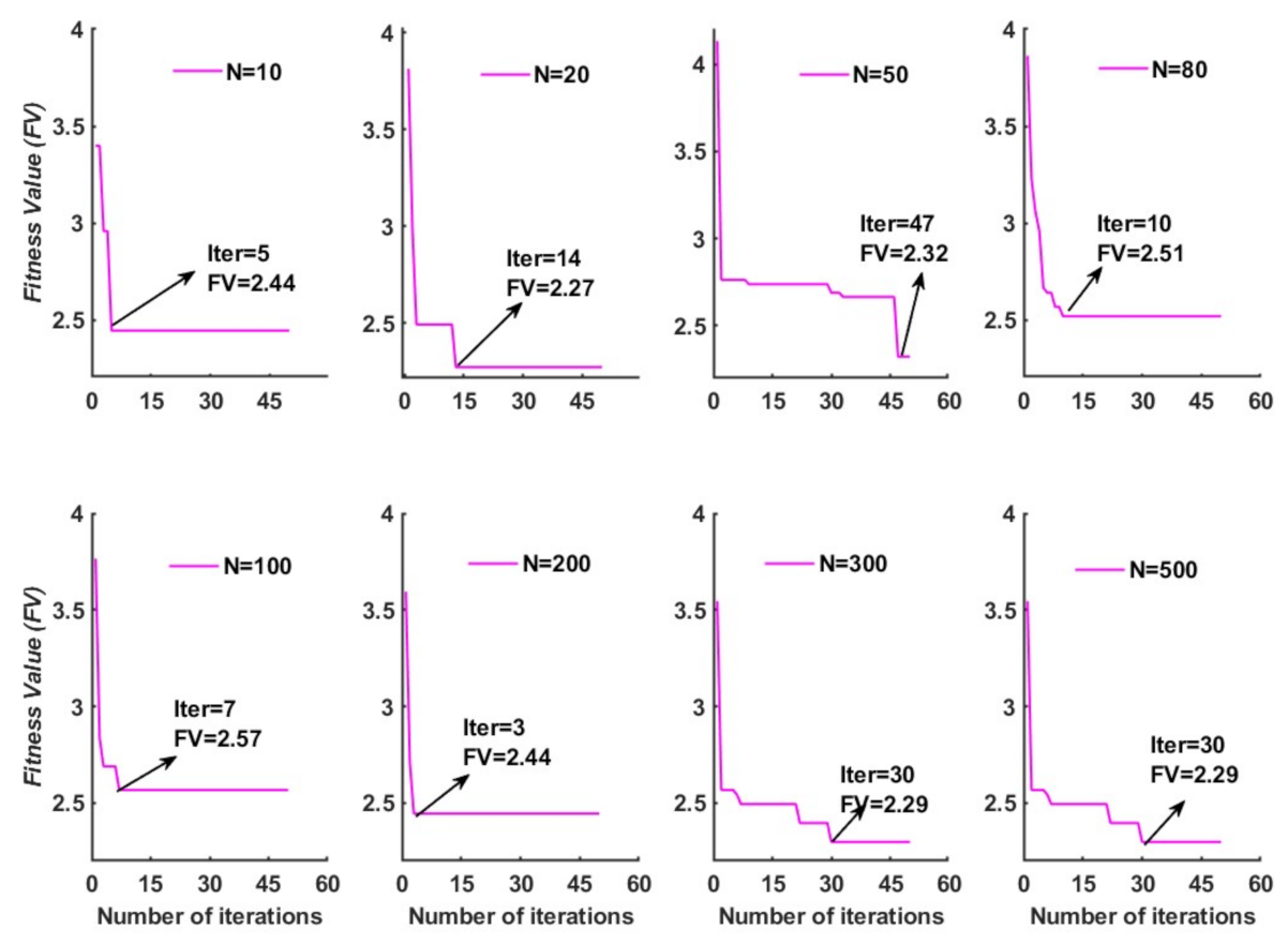
2.1. Manta Ray Foraging Optimization (MRFO)

To develop the proposed DL, hybrid stacked LSTM sequence to sequence autoencoder (i.e., SAELSTM) model, we have adopted the Manta Ray Foraging Optimization (MRFO) method for feature selection. The MRFO is a bio-inspired novel algorithm that simulates the intelligent foraging behaviors of manta rays and the characteristics of their foraging behaviors [57]. The concept is applicable to our present solar radiation prediction problem given that the manta rays, on which the MRFO is based, have three distinct foraging strategies that they use to search for food, which form the fundamental search schemes of the MRFO to optimize the solution of our proposed solar radiation prediction problem.

• Chain foraging: When 50 or more manta rays begin foraging, they line up one after the other, forming an ordered line. Male manta rays are smaller than females and dive on top of their back stomachs to the beats of the female’s pectoral fins. As a result, plankton (prey or marine drifters) lost by past manta rays will be scooped up by those after them. Through working together in this manner, they can get the most plankton into their gills and increase their food rewards. This mathematical model of chain foraging is represented as follows [58]:

  $$M_m^{*}=\left\{\begin{array}{cc}{M}_m+(M_B-M_m)(r+\sigma )\hfill & \hfill \mathrm{if}m=1\\ M_m+r(M_{m-1}-M_m)+\sigma (M_B-M_m)\hfill & \hfill \mathrm{if}m\ne 1\end{array}\right.$$

  (1)

  $$\sigma =2r\sqrt{|log(r\left)\right|)}$$

  (2)

  where ($M_m$) = individual manta ray (m); r = random uniformly distributed number in $[0,1]$. $M^{*}$ and MB = new or best position of manta ray in population, $\sigma$ = weight coefficient as a function of each iteration.
  It is clear from Equation (1) that the previous manta ray in the chain and the spatial location of the strongest plankton clearly define the position update process in chain foraging.
• Cyclone foraging: When the abundance of plankton is very high, hundreds of manta rays group together in a cyclone foraging strategy. Their tail ends spiral along with the heads to form a spiraling vertex in the cyclone’s eye, and the purified water rises to the surface. This attracts plankton to their open mouths. Mathematically, this cyclone foraging is divided into two parts. The first half focuses on enhancing the exploration and is updated as [59]:

  $$M_m^{*}=\left\{\begin{array}{cc}{M}_R+(M_R-M_m)(r+\beta )\hfill & \hfill \mathrm{if}m=1\\ M_m+r_1(M_{m-1}-M_m)+\beta (M_R-M_m)\hfill & \hfill \mathrm{if}m\ne 1\end{array}\right.$$

  (3)

  where $M_R$ = individual created randomly:

  $$M_R=M^{min}+r_1(M^{max}-M^{min}).$$

  (4)
  The adaptive weight coefficient ($\beta$) is varied as:

  $$\beta =2e^{r_2\frac{{\mathit{Iter}}_m-{\mathit{Iter}}_m+1}{{\mathit{Iter}}_m}}sin\left(2\pi r_2\right)$$

  (5)

  where $\mathit{Iter}$ = current iteration and random uniformly distributed number, and $r_2$ is over $[0,1]$.
  The second half concentrates on improving the exploitation, so the update is as per:

  $$M_m^{*}=\left\{\begin{array}{cc}{M}_B+(M_B-M_m)(r_1+\beta )\hfill & \hfill \mathrm{if}m=1\\ M_B+r_1(M_{m-1}-M_m)+\beta (M_B-M_m)\hfill & \hfill \mathrm{if}m\ne 1.\end{array}\right.$$

  (6)
• Somersault foraging: This is the final foraging strategy with manta rays discovering the food supply and doing backwards somersaults to circle the plankton for attraction. Somersaulting is a spontaneous, periodic, local, and cyclical action that manta rays use to maximize their food intake. The third strategy is where an update of each individual occurs around an optimal position [60]:

  $$M_m^{*}=M_m+S(r_3{M}_B-r_4{M}_m).$$

  (7)
  In Equation (7), S = somersault coefficient ($S=2$) controlling the domain of manta rays, $r_3$ and $r_4$ are random numbers within $[0,1]$.

Based on a randomly generated number, the MRFO algorithm will switch between chain foraging and cyclone foraging [60,61]. Then, summersault foraging takes action to update individuals’ existing positions using the best solution available at the time. These three distinct foraging processes are used interchangeably to achieve the global optimum solution of the optimization problem, thus satisfying the predefined termination criterion.

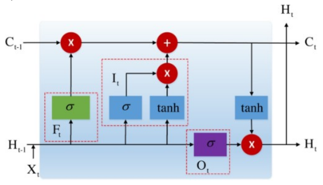
2.2. Long Short-Term Memory Network (LSTM)

Recurrent Neural Networks (RNN) have lately been researched to accomplish the prediction problem due to the rapid development of DL, the rise of computation skills [45,51,52,62], and the failure of traditional ML methods to effectually reveal the intrinsic association between time-series data [63]. RNN has a short-term memory based on its recurring process in hidden layers correlating with contextual information. Furthermore, because of the issue related with gradient vanishing and explosion, RNNs are unable to provide long-term memory [64]. Hence, a Long Short-Term Memory network (LSTM) is proposed by researchers and has been used extensively in time-series prediction. LSTM is an RNN deformation structure that controls the memory information of time-series data by adding memory cells to the hidden layer. Information is passed between cells in the hidden layer by means of a series of programmable gates (input, output, and forget gate) [65]. LSTM can maintain the cell state through its gate mechanism, which can solve both short-term and long-term memory reliance problems, thus avoiding the vanishing gradient and explosion problem.

Figure 1 depicts the basic LSTM cell with three gates in a memory cell. The function of input gates is to keep track of the most recent information in a memory cell; the output gate function is to maintain control over the dissemination of the most up-to-date information throughout the remainder of the networks. The third gates (forget gates) function is to determine if the information should be deleted based on the status of the preceding cell. The equations below (8)–(15) explain how to implement and update the LSTM cell state and compute the LSTM outputs.

$$F_t=\sigma (W_{xf}{X}_t+W_{hf}{H}_{t-1}+B_f)$$

(8)

$$I_t=\sigma (W_{xi}{X}_t+W_{hi}{H}_{t-1}+B_i)$$

(9)

$${\overline{C}}_t=\sigma (W_{xc}{X}_t+W_{hc}{H}_{t-1}+B_c)$$

(10)

$$C_t=F_t\ast C_{t-1}+I_t\ast {\overline{C}}_t$$

(11)

$$O_t=\sigma (W_{xo}{X}_t+W_{ho}{H}_{t-1}+B_o)$$

(12)

$$H_t=o_{t}tanh\left(C_t\right)$$

(13)

$$Y_t=\sigma (W_{hy}{H}_t+B_y)$$

(14)

$$\sigma \left(x\right)=\frac{1}{1+{exp}^{-x}}$$

(15)

where $X_t$ = input vector; $Y_t$ = output vector; $I_t$ = input gate outcome; $F_t$ = forget gate outcome; $O_t$ = output gate outcome; $C_t$ = finishing state in memory block; ${\overline{C}}_t$ = temporary; $\sigma$ = sigmoid function; $W_{xf}$, $W_{xi}$, $W_{xc}$, and $W_{xo}$ are input weight matrices; $W_{hf}$, $W_{hi}$, $W_{hc}$, and $W_{ho}$ are recurrent weight matrices; $W_{hy}$ is output weight matrix; and $B_f$, $B_i$, $B_c$, $B_o$, and $B_y$ are the related bias vectors.

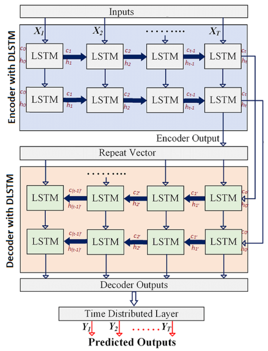
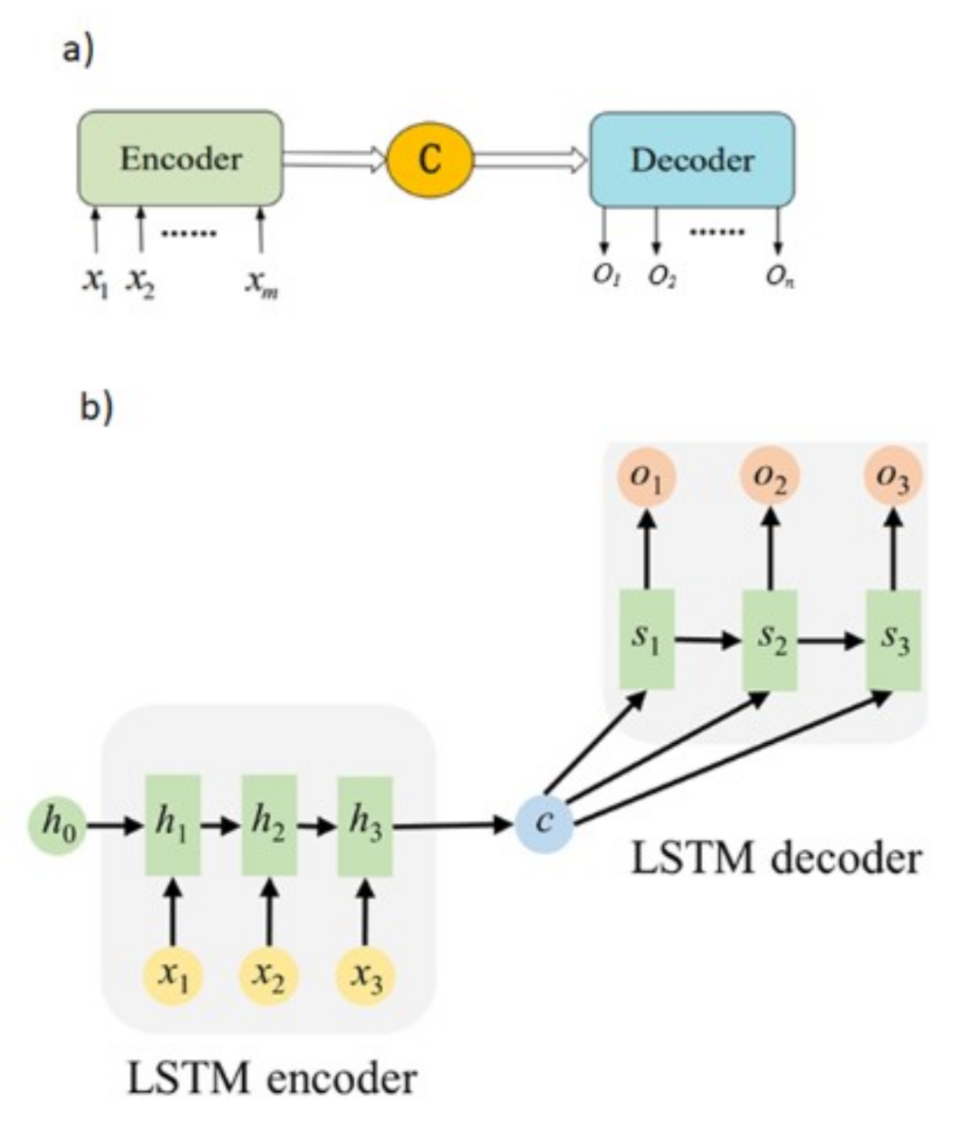
2.3. Stacked LSTM Sequence-to-Sequence Autoencoder (SAELSTM)

Our proposed DL hybrid stacked LSTM sequence-to-sequence autoencoder (i.e., SAELSTM) model has used the approach of Cho et al. [66], who introduced an RNN encoder–decoder network. This serves as a prototype for a sequence-to-sequence (seq2seq) model. The Seq2seq paradigm has recently become popular in the field of machine translation [67,68,69] and is made up of two parts: an encoder and a decoder, as illustrated in Figure 2a. Data are received by the encoder, which compresses it into a single vector. The vector at this point is known as a context vector, and the decoder uses it to create an output sequence. RNN or LSTM is used by the encoder to transform input into a hidden state vector. The encoder’s output vector is the latest RNN cell’s hidden state. The encoder sends the context vector to the decoder. The encoded context vector is utilized as the decoder network’s starting hidden state, and the output value of the previous time step is sent into the next LSTM unit as an input for progressive prediction.

Mathematically, an encoder $\varphi$ is formed by the input layer and the hidden layer, which compresses input data x from a high-dimensional representation into a low-dimensional representation Z. In the meantime, a decoder $\Psi$ is formed by the hidden layer and the output layer, which reconstructs the input data $x^{\prime }$ from the appropriate codes. These transitions in the seq2seq learning can be signified mathematically by the standard neural network function passed through a sigmoid activation function $\sigma$ (Equation (15)).

$$\begin{array}{cc}\hfill \varphi :X& \to Z\hfill \\ \hfill x& \mapsto \varphi \left(x\right)=\sigma (Wx+b):=z\hfill \end{array}$$

(16)

$$\begin{array}{cc}\hfill \Psi :Z& \to Z\hfill \\ \hfill z& \mapsto \Psi \left(x\right)=\sigma (\tilde{W}z+\tilde{b}):=x^{\prime }\hfill \end{array}$$

(17)

where W is weight matrices and b is the bias.

The encoder and decoder networks of the LSTM seq2seq model utilized in this study for GSR prediction are shown in Figure 2b. To use this seq2seq learning in GSR prediction, LSTM layers were stacked on the encoder and decoder parts of the model and called the stacked LSTM sequence-to-sequence autoencoder (SAELSTM). By stacking LSTMs, we may be able to improve our model’s prediction capability to comprehend more complicated representations of our time-series data in hidden layers by collecting information at various levels [70]. Moreover, on the figure, x and o are the input data and output data, c = encoder context vector and ht and st = hidden states in the encoder and decoder, which are respectively as follows:

$$h_t=LST{M}_{enc}(x_t,h_{t-1})$$

(18)

$$h_t=LST{M}_{dec}(o_{t-1},s_{t-1}).$$

(19)

Each encoder LSTM layer calculates context vector c, and this context vector will be replicated and sent to each decoder unit.

2.4. Benchmark Models

To validate the proposed deep learning hybrid stacked LSTM sequence-to-sequence autoencoder (i.e., SAELSTM) model, we adopted popular Machine Learning models: (i) Deep Neural Networks (DNN) as extensions of artificial neural network ([43,71,72,73,74,75,76,77]), (ii) Gradient Boosting Regressor (GBM) as an ensemble-based Machine Learning model [78,79,80,81], (iii) Random Forest Regression (RFR) as an ensemble-based Machine Learning model that uses an ensemble of Decision Trees to predicts outcomes [82,83,84,85,86,87,88,89,90], (iv) Extremely Randomized Trees Regression model (ETR) that uses bagging [91], and (v) the Adaptive Boosting Regression (ADBR) that aims to adaptively solve complex problems [10,92,93,94,95,96].

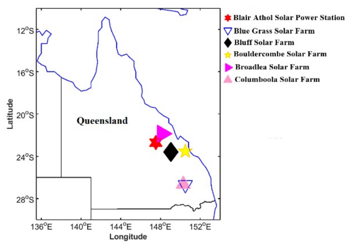
3. Study Area and Data Available

The proposed DL hybrid stacked LSTM sequence-to-sequence autoencoder (i.e., SAELSTM) model was built for Queensland, which is a region known as Australia’s sunshine state with 300 days of sunshine per year, a tropical climate, 8 to 9 h of sunshine per day, and average maximum and minimum temperatures of 25.3 and 15.7 °C, respectively [97]. As of March 2021, there are currently 44 large-scale renewable energy projects in Queensland (operating, under construction or financially committed). This roughly equates to an investment of $9.9 billion or 7000 construction jobs, or 5156 megawatts (MW) of renewable energy, and 12.6 million tons of carbon that can be saved per year. The state now has 6200 MW of renewable energy capacity, including rooftop solar PV and accounts for about 20% of total power consumption [98]. In this study, six solar farms in Queensland, Australia, ranging in size from 60 to 280 MW, were chosen for the study. The Bouldercombe solar farm (proposed to be developed by Eco Energy World) located 20 km southwest of Rockhampton, Queensland with 280 MW capacity. This solar farm will utilize 90,000 PV on a one-axis tracking system to capture the sun energy. The Bluff solar farm (proposed) entails the building of a 332 hectare (ha) solar farm with a capacity of 250 MW, which will generate power using PV panels with rotating axes to capture solar energy and transfer it to the local electrical grid through transmission lines.

The Blue Grass solar farm project site is 14 km from Chinchilla in Queensland, which is planned to be in the fully operational stage by the fourth quarter of 2021. This 200 MW solar farm will provide 420 Gigawatt hours (GWh) of green electricity per year, which is enough to power about 80,000 Queensland households. The Columboola Solar Farm (under construction by Sterling & Wilson) with 162 MW capacity project on 410 ha of grazing land is located in Queensland’s Western Downs and will utilize 407,171 next-generation bifacial solar panels that produce energy from the sun using both sides of the panel. Planned to be completed in 2022, the Columboola Solar Farm will generate approximately 440 GWh of renewable energy per year, which is enough renewable energy to power 75,000 homes for 35 years. The Broadlea and Blair Athol solar farms (both proposed) with a capacity of 100 MW and 60 MW are located at Blair Athol and Broadlea of North Queensland, respectively [99]. The study site details (the statistics of GSR) are shown in

Table 1. Statistical summary of daily global solar radiation (GSR; MJm${}^{-2}$day${}^{-1}$) in solar energy farms for Queensland Australia where the proposed deep learning hybrid SAELSTM model is implemented.

Property	Blair Athol Solar Power Station	Blue Grass Solar Farm	Bluff Solar Farm	Bouldercombe Solar Farm	Broadlea Solar Farm	Columboola Solar Farm
Latitude	22°41${}^{\prime }$28${}^{″}$ S	26°40${}^{\prime }$48${}^{″}$ S	23°35${}^{\prime }$53${}^{″}$ S	23°31${}^{\prime }$30${}^{″}$ S	21°51${}^{\prime }$43${}^{″}$ S	26°38${}^{\prime }$10${}^{″}$ S
Longitude	147°32${}^{\prime }$31${}^{″}$ E	150°29${}^{\prime }$35${}^{″}$ E	149°02${}^{\prime }$20${}^{″}$ E	150°29${}^{\prime }$56${}^{″}$ E	148°10${}^{\prime }$12${}^{″}$ E	150°17${}^{\prime }$46${}^{″}$ E
Capacity (MW)	60	200	250	280	100	162
Median	20.00	19.00	20.00	20.00	20.00	19.00
Mean	20.02	19.28	19.76	19.57	19.85	19.33
Standard deviation	5.80	6.43	5.84	5.83	5.68	6.48
Variance	33.64	41.34	34.10	33.95	32.23	42.05
Maximum	32.00	32.00	32.00	32.00	31.00	33.00
Minimum	4.00	4.00	4.00	4.00	3.00	4.00
Mode	28.00	28.00	28.00	28.00	28.00	29.00
Interquartile range	8.00	9.00	8.00	8.00	8.00	9.00
Skewness	−0.38	−0.18	−0.36	−0.36	−0.41	−0.19
Kurtosis	2.65	2.34	2.57	2.54	2.65	2.34

, and their locations are shown in Figure 3.

In the supervised learning process, the predictive model is presented with example inputs (predictors) and their desired outputs (predictands), and the goal is to learn a general rule that maps inputs to outputs. Since GSR prediction is the supervised learning, we need the predictors and predictand. Therefore, this study has used the Global Climate Models (GCM) meteorological data (cloud parameters, humidity parameters, precipitation, wind speed, etc.) and ground-based observation data (Evaporation, Vapor Pressure, Relative Humidity at maximum and minimum temperature, Rainfall, Maximum and Minimum Temperature) from Scientific Information for Landowners (SILO) as the predictors. As the GSR (predictands or target) measurements for each site’s precise latitude and longitude are not publicly accessible, ground truth observations are obtained from the SILO database.

The Department of Science, Information Technology, Innovation and Arts under Queensland Government (DSITIA) manages the Long Paddock SILO database [100]. GCM outputs are collected from the online archive (Centre for Environmental Data Analysis) hosting CMIP5 project’s GCM output collection [101]. We adopt data from CSIRO-BOM ACCESS1-0 (grid size 1.25° × 1.875°) [102], MOHC Hadley-GEM2-CC (grid size 1.25° × 1.875°) [103], and the MRI MRI-CGCM3 (grid size 1.12148° × 1.125°) [104] with historical outputs spanning 1950-01-01T12:00:00 and 2006-01-01T00:00:00 indexed by longitude, latitude, time, atmospheric pressure (8 levels), or near-surface readings.

Table 2. Predictor variables for daily GSR. (a) Atmospheric variables from global climate models and (b) Ground-based observational climate data from Scientific Information for Landowners (SILO) used to train the proposed Deep Learning hybrid SAELSTM model.

	Variable	Description	Units
Global Circulation Model Atmospheric Predictor Variables	clt	Cloud Area Fraction	%
	hfls	Surface Upward Latent Heat Flux	wm${}^{-2}$
	hfss	Surface Upward Sensible Heat Flux	wm${}^{-2}$
	hur	Relative Humidity	%
	hus	Near-Surface Specific Humidity	gkg${}^{-1}$
	pr	Precipitation	kgm${}^{-2}$s${}^{-1}$
	prc	Convective Precipitation	kgm${}^{-2}$s${}^{-1}$
	prsn	Solid Precipitation	kgm${}^{-2}$s${}^{-1}$
	psl	Sea Level Pressure	pa
	rhs	Near-Surface Relative Humidity	%
	rhsmax	Surface Daily Max Relative Humidity	%
	rhsmin	Surface Daily Min Relative Humidity	%
	sfcWind	Wind Speed	${\mathrm{ms}}^{-1}$
	sfcWindmax	Daily Maximum Near-Surface Wind Speed	ms${}^{-1}$
	ta	Air Temperature	K
	tas	Near-Surface Air Temperature	K
	tasmax	Daily Max Near Surface Air Temperature	K
	tasmin	Daily Min Near Surface Air Temperature	K
	ua	Eastward Wind	ms${}^{-1}$
	uas	Eastern Near-Surface Wind	ms${}^{-1}$
	va	Northward Wind	ms${}^{-1}$
	vas	Northern Near-Surface Wind	ms${}^{-1}$
	wap	Omega (Lagrangian Tendency of Air Pressure)	pas${}^{-1}$
	zg	Geopotential Height	m
Grnd.-based SILO	T.Max	Maximum Temperature	K
	T.Min	Minimum Temperature	K
	Rain	Rainfall	mm
	Evap	Evaporation	mm
	VP	Vapor Pressure	Pa
	RHmaxT	Relative Humidity at Maximum Temperature	%
	RHminT	Relative Humidity at Minimum Temperature	%

provides a brief overview of each of the meteorological variables comprised in the dataset. This final dataset contained 20,455 × 75).

4. Predictive Model Development

Predictive models with time-series data require cleaning and filtering. Normalization of input variables, sometimes accomplished by scaling, is crucial in Machine Learning [105]. The intent of this normalization implementation is to eliminate the potential for numerically prominent variables to be favored over variables with miniature figures. Additionally, because kernel quantities rely largely on input vectors’ internal multiplication, there are calculation complications arising from large input variables [106]. Therefore, to overcome numerical complexities during modeling, the normalization of input vectors is essential. In this study, Equation (20) is applied so that each input variable is scaled linearly to a range [0, 1] [107].

$$x_i^n=\frac{x_i-x_{min}}{x_{max}-x_{min}}$$

(20)

where $x_i$ = input vector; the minimum and maximum of measured data are $x_{min}$ and $x_{max}$ is the scaled version of $x_i$.

One of the fundamental concepts in the fields of Machine Learning and data mining is the concept of feature selection (FS), which enhances the performance of predictive models tremendously [17]. Furthermore, FS allows for the removal of irrelevant or partially relevant features, which in turn improves the performance of models [105]. In the course of time, researchers have applied several meta-heuristic optimization techniques for the purposes of FS, which overcome the limitations of traditional optimization techniques. Therefore, in this study, a new FS method based upon a meta-heuristic algorithm called Manta Ray Foraging Optimization (MRFO) was used. This MRFO mimics the feeding behavior of manta rays, which are one of the largest marine animals and explained in Section 2.1.

In FS techniques, one aspect that is critical is evaluation of the selected feature. As the proposed MRFO is a wrapper-based approach to FS, the evaluation process entails a learning algorithm (regressor). For this purpose, we used a known regression method, K-Nearest Neighbor (KNN). In general, FS is designed with two objectives: higher accuracy and a lower number of selected features. The combination of higher accuracy and fewer features selected indicate that the chosen subset is more accurate. This study has taken these two characteristics into account when creating the fitness function for our proposed MRFO FS. Due to the need to minimize the features, the root mean square error (RMSE), which is a complementary measure of regression accuracy, was selected. In this study, after normalizing all predictor variables, the MRFO FS algorithm is run with the following configurations:

• Population size $N=[10,20,50,80,100,200,300,500]$.
• The number of maximum iterations (T) = 50.
• Somersault coefficient (S) = 2.

Similarly, we observed an effect of population size on MRFO performance in terms of root mean square error (fitness value, FV). To achieve this, we evaluated the proposed approaches for population sizes of 10, 20, 50, 80, 100, 200, 300, and 500. The convergence graph (Figure 4) shows the impact of different population sizes on FV for the Broadlea solar farm. From the convergence graph, it is apparent that increasing the size of the population is not always beneficial to FV. Along with this, the higher population size is computationally inefficient.

Therefore, for all other five solar farms, the value of the population size is set to 20 to balance the FV with the algorithm computation time. With this MRFO FS process, 16 meteorological predictors from the pool of 75 (data: 20,455 × 16) are selected for Blair Athol solar power station, Bluff solar farm, and Bouldercombe solar farm. Whereas for the Blue Grass solar farm and Columboola solar farm, 17 meteorological predictors (data: 20,455 × 17) are selected. Similarly, for the Broadlea solar farm, only 13 meteorological predictors (Data: 20,455 × 13) are selected. The predictors from the MRFO feature selection process for the prediction of GSR for all six solar farms are shown in

Table 3. The selected predictor (input) variable using Manta Ray Foraging Optimization (MRFO) feature selection for the proposed deep learning hybrid SAELSTM model. For abbreviations, readers should refer to Table 2 (example: $hu{r}_{1000}=$ relative humidity 1000 hPa pressure height).

Blair Athol Solar Power Station	Blue Grass Solar Farm	Bluff Solar Farm	Bouldercombe Solar Farm	Broadlea Solar Farm	Columboola Solar Farm
Evap	Evap	Evap	Evap	Evap	Evap
RHmaxT	RHmaxT	RHmaxT	RHmaxT	RHmaxT	RHmaxT
hfss	ua_1000	hfss	hfss	hfss	ua_1000
hur_1000	hfls	hur_1000	Rain	hur_1000	hfls
ua_5000	hfss	ua_5000	ua_1000	Rain	hfss
wap_1000	hus_5000	wap_1000	zg_1000	T.Max	hus_5000
Rain	ta_25000	hus_5000	hus_5000	RHminT	wap_1000
T.Max	wap_1000	sfcWindmax	wap_1000	wap_85000	ta_25000
va_85000	wap_85000	Rain	va_85000	wap_1000	Rain
RHminT	sfcWindmax	T.Max	T.Max	va_85000	hur_1000
wap_85000	zg_1000	ta_25000	hur_1000	ua_5000	ua_5000
zg_5000	Rain	wap_85000	ta_25000	va_50000	wap_85000
va_50000	RHminT	zg_1000	wap_85000	zg_5000	RHminT
sfcWindmax	ua_5000	RHminT	ua_5000		sfcWindmax
hus_5000	T.Max	va_50000	sfcWindmax		T.Max
hfls	va_25000	zg_85000	va_50000		zg_1000
	hur_1000				va_25000

.

Table 3 reveals that the optimal set of meteorological predictors are somewhat site-specific as the MRFO feature selection method selects different predictors for the different study sites. For example, 16 predictors (in a different order) are selected for the Blair Athol solar power station, whereas for the Blue Grass solar farm, there are 17 predictors, and for the Bluff Solar Farm, we have 16 best predictors. Interestingly, for the Broadlea solar farm, the MRFO feature selection process resulted in 13 meteorological predictors, and for the Columboola solar farm, there were 17 predictor variables—again in different order or predictor type. While the exact cause of these diverse list of screened predictors is not clear, it is possible that the strength of the features related to the measured GSR are different for the different study sites.

Lastly, before feeding the data into the ML model, training and testing data are created for the purpose of predicting daily GSR. Training datasets are used to train a model, and testing datasets are used to estimate the model’s range of capability. Throughout previous research, it was found that 70-30 % was usually used for data division during training and testing, and that there is no standard way of dividing data. In this study, for training, 54 years of data are used (20,089 data points), validation uses 20% of the data in the training set (4018 data points), and testing uses 1 year of data (365 data points). Moreover, to prevent look-ahead bias, only the training set was used for optimization, and the testing set was only used to test the model’s performance to predict the daily GSR.

4.1. Stacked LSTM Sequence to Sequence Autoencoder Model Development

As mentioned in Section 2.3, this study utilizes the LSTM-based seq2seq model in prediction of GSR for six solar farms of Queensland, Australia. Furthermore, we have added two layers: namely, a repeat vector layer and a time-distributed dense layer in the SAELSTM model. The repeat vector layer repeats the context vector received from the encoder and feeds it to the decoder as an input. This is repeated for n steps, where n is the number of future steps that must be predicted [108].

Similarly, to maintain one-to-one relationships on input and output, we have employed a wrapper layer called a time-distributed dense layer. Furthermore, the flattened output of the decoder is mixed with the time steps if a time-distributed dense layer is not utilized for sequential data. However, if this layer is used, the output for each time step is received individually. In particular, the LSTM encoder extracts features from predictor variables and then passes on the hidden state of its last time step to the LSTM decoder. Each output time step contains the future variables. The LSTM decoder output is transformed directly by a fully connected time-wrapped layer to predict output at each subsequent step. The proposed methodology step-wise is shown in Figure 5.

• The encoder layer of the SAELSTM receives as an input a sequence X of predictor variables after MRFO FS, which are represented as $X_{ij}$ with $i=1,\dots ,l$ terms to time series in $j=1,\dots ,t$ time step.
• The encoder recursively handles the input sequence (X) of length t. Then, it updates the cell memory state vector $C_t$ and hidden state vector $h_t$ at time step t. Afterwards, the encoder summarizes the input sequence in $C_t$ and $h_t$.
• An encoder output is fed through a repeat vector layer, which is then fed into a decoder layer.
• Afterwards, the decoder layer of SAELSTM adopts Ct and ht from an encoder as initial cell memory state vector. The initial hidden state vectors C0’ and h0’ for t’ length are at the respective time step.
• Afterwards, the decoder layer of SAELSTM uses the final vectors Ct and ht passed from the encoder as initial cell memory state vectors and initial hidden state vectors C0’ and h0’ for t’ length of time step.
• The learning of features is performed by the decoder as included in the original input to generate multiple outputs with N-time step ahead.
• Using a time-distributed dense layer, each time step has a fully connected layer that separates the outputs (GSR). The prediction accuracy of the SAELSTM model can be evaluated here.

It is vital to select hyperparameters sensibly when designing an ML model in order to achieve optimal performance. For example, hyperparameters include the optimization and tuning of model structures, the step size of a gradient-based optimization, and data presentation, all of which have significant effects on the learning process. A grid search method based on five-fold cross-validation was utilized to optimize all the hyperparameters in the SAELSTM model. During SAELSTM model training, the activation function ‘ReLU’ is applied to the LSTM layers to handle vanishing gradients, allowing learning to be more rapid and effective [109]. Furthermore, Adam is chosen as the optimization algorithm with a constant learning rate of (lr) 0.001; decay rate ${\beta }_1=0.9$ & ${\beta }_2=0.9999$ and epsilon ($ϵ$) of ${10}^{-8}$. The Adam optimization algorithm is computationally efficient, has a reasonable memory requirement, is invariant to gradient rescaling, and is well-suited to handling large datasets [110]. Additionally, the regularization method called early stopping (es) [111] is used in developing predictive models, which quits the training process by controlling validation loss before a certain number of iterations.

During model development, this study also uses the ‘ReduceLROnPlateau’ scheduler, which reduces the learning rate when a validation loss stops improving. As a start, ‘ReduceLROnPlateau’ uses the default learning rate of the optimizer (0.001). It is configured with patience (number of epochs with no improvement before the learning rate is reduced) of 8 and a factor of ($lrnew=lr\ast factor$) 0.2.

Table A1. (a) The proposed Deep Learning hybrid SAELSTM (i.e., stacked LSTM sequence-to-sequence autoencoder) and Deep Neural Network (DNN) models. (b) The comparison of machine learning models: Random Forest Regression (RFR), Adaboost Regression (ADBR), Gradient Boosting Machine (GBM), and Extremely Random Tree Regression (ETR). Note: ReLU = Rectified Linear Units.

Predictive Models	Model Hyperparameters	Hyperparameter Selection	Blair Athol Solar Power Station	Blue Grass Solar Farm	Bluff Solar Farm	Bouldercombe Solar Farm	Broadlea Solar Farm	Columboola Solar Farm
SAELSTM	Encoder LSTM cell 1	[10,20,30,40,50,60]	20	10	30	20	40	20
	Encoder LSTM cell 2	[5,10,15,25]	10	5	25	15	25	15
	Encoder LSTM cell 3	[6,8,10,15]	6	6	10	15	15	10
	Decoder LSTM cell 1	[80,90,100,200]	100	80	200	100	100	90
	Decoder LSTM cell 2	[40,50,60,70,100]	70	60	50	100	60	50
	Decoder LSTM cell 3	[5,10,15,20,25,30]	20	15	25	15	30	15
	Activation function	ReLU
	Epochs	[300,400,500,600,700]	400	500	300	500	400	500
	Drop rate	[0,0.1,0.2]	0.1	0.2	0	0	0.2	0.1
	Batch Size	[5,10,15,20,25,30]	10	15	15	20	10	10
DNN	Hiddenneuron 1	[100,200,300,400,50]	300	100	100	200	100	200
	Hiddenneuron 2	[20,30,40,50,60,70]	60	70	40	50	30	20
	Hiddenneuron 3	[10,20,30,40,50]	40	30	50	20	10	40
	Hiddenneuron 4	[5,6,7,8,12,15,18]	15	18	7	12	15	18
	Epochs	[100,200,400,500]	500	200	100	200	100	400
	Batch Size	[5,10,15,20,25,30]	5	10	20	15	15	20
Predictive Models	Model hyperparameters	Hyperparameter Selection	Blair Athol Solar Power Station	Blue Grass Solar Farm	Bluff Solar Farm	Bouldercombe Solar Farm	Broadlea Solar Farm	Columboola Solar Farm
RFR	The maximum depth of the tree	[5,8,10,20,25]	20	25	8	25	20	10
	The number of trees in the forest	[50,100,150,200]	150	100	50	100	50	200
	Minimum number of samples to split an internal node	[2,4,6,8,10]	6	8	10	10	8	10
	The number of features to consider when looking for the best split.	[’auto’, ’sqrt’, ’log2’]	auto	auto	auto	auto	auto	auto
ADBR	The maximum number of estimators at which boosting is terminated	[50,100,150,200]	150	200	100	150	200	150
	learning rate	[0.01,0.001,0.005]	0.01	0.001	0.01	0.01	0.005	0.001
	The loss function to use when updating the weights after each boosting iteration	[‘linear’, ‘square’, ‘exponential’]	square	square	square	square	square	square
GBM	Number of neighbors	[5,10,20,30,50,100]	50	30	20	30	50	20
	Algorithm used to compute the nearest neighbors	[‘auto’, ‘ball_tree’, ‘kd_tree’, ‘brute’]	auto	auto	auto	auto	auto	auto
	Leaf size passed to BallTree or KDTree	[10,20,30,50,60,70]	10	30	20	10	30	10
ETR	The number of trees in the forest	[10,20,30]	30	10	10	20	30	20
	The maximum depth of the tree	[5,8,10,20,25]	8	10	5	8	10	5
	The number of features to consider when looking for the best split	[’auto’, ’sqrt’, ’log2’]	auto	auto	auto	auto	auto	auto
	Minimum number of samples to split an internal node	[5,10,15,20]	15	10	20	15	20	15

(in the Appendix A) lists the search space and optimized results. Figure 6 illustrates that the training and validation losses of the SAELSTM model with optimum parameters (Broadlea solar farm gradually) decrease as the epoch increases, indicating the satisfactory performance of the SAELSTM training.

4.2. Benchmark Model Development

We compared the proposed deep learning hybrid stacked LSTM sequence-to-sequence autoencoder (i.e., SAELSTM) model with five forecast models: Deep Neural Network (DNN), Gradient Boosting Regression (GBM), Random Forest Regression (RFR), Extremely Randomized Trees (ETR), and Adaptive Boosting Regression (ADBR) were performed to validate its predictive efficacy. All the proposed (SAELSTM) as well as benchmark models were built using Python under the framework of Keras 2.2.4 [112,113] on TensorFlow 1.13.1 [114,115]. The hyperparameters of the benchmark models are also derived by using grid search (see Table A1 in Appendix A). The training process of all the models was conducted on a system that has the CPU type of Intel®Core™i7 with 32GB RAM.

4.3. Performance Evaluation Metrics Considered

In the past, several approaches have been used to evaluate model efficiency. However, since each metric has its own strengths and weaknesses, the current study uses a collection of common statistical metrics approaches (e.g., Correlation (r), root mean square error (RMSE), mean absolute error (MAE), relative root mean square error (RRMSE), relative mean absolute error (RMAE), Willmott’s Index (WI), Nash–Sutcliffe Equation (NS), Legates and McCabe’s (LM), and Explained Variance Score ($E_{var}$)) represented below [51,53,54,105,106,116,117,118,119,120,121] in Equations (21)–(31).

$$r=\frac{{\sum }_{i=1}^n({\mathit{GSR}}^m-\langle {\mathit{GSR}}^m\rangle )({\mathit{GSR}}^p-\langle {\mathit{GSR}}^p\rangle )}{\sqrt{{\sum }_{i=1}^n{({\mathit{GSR}}^m-\langle {\mathit{GSR}}^m\rangle )}^2}\sqrt{{\sum }_{i=1}^n{({\mathit{GSR}}^p-\langle {\mathit{GSR}}^p\rangle )}^2}}$$

(21)

$$\mathit{RMSE}=\sqrt{\frac{1}{n}\sum _{i=1}^n{({\mathit{GSR}}^p-{\mathit{GSR}}^m)}^2}$$

(22)

$$\mathit{MAE}=\frac{1}{n}\sum _{i=1}^n|{\mathit{GSR}}^p-{\mathit{GSR}}^m|$$

(23)

$$\mathit{RRMSE}=\frac{\sqrt{\frac{1}{n}{\sum }_{i=1}^n{({\mathit{GSR}}^p-{\mathit{GSR}}^m)}^2}}{\langle {\mathit{GSR}}^m\rangle }$$

(24)

$$\mathit{RMAE}=\frac{1}{n}\sum _{i=1}^n\frac{|{\mathit{GSR}}^p-{\mathit{GSR}}^m|}{{\mathit{GSR}}^p}$$

(25)

$$\mathit{WI}=1-\frac{{\sum }_{i=n}^n{({\mathit{GSR}}^m-{\mathit{GSR}}^p)}^2}{{\sum }_{i=n}^n\left(\right|{\mathit{GSR}}^p-\langle {\mathit{GSR}}^m\rangle |+|{\mathit{GSR}}^m-\langle {\mathit{GSR}}^m\rangle {\left|\right)}^2}$$

(26)

$$\mathit{NSE}=1-\frac{{\sum }_{i=1}^n{({\mathit{GSR}}^m-{\mathit{GSR}}^p)}^2}{{\sum }_{i=1}^n{({\mathit{GSR}}^m-\langle {\mathit{GSR}}^m\rangle )}^2}$$

(27)

$$\mathit{LM}=1-\frac{{\sum }_{i=1}^n|{\mathit{GSR}}^m-{\mathit{GSR}}^p|}{{\sum }_{i=1}^n|{\mathit{GSR}}^m-\langle {\mathit{GSR}}^m\rangle |}$$

(28)

$$E_{\mathit{var}}=1-\frac{Var({\mathit{GSR}}^m-{\mathit{GSR}}^p)}{Var\left({\mathit{GSR}}^m\right)}$$

(29)

$$\mathit{SS}=1-\frac{\mathit{RMSE}(p,x)}{\mathit{RMSE}(pr,x)}$$

(30)

$${\mathit{RMSE}}_r=\frac{\mathit{RMSE}(p,x)}{\mathit{RMSE}(r,x)}$$

(31)

where ${\mathit{GSR}}^m$ and ${\mathit{GSR}}^p$ are the observed and predicted value of GSR, $\langle {\mathit{GSR}}^m\rangle$ and $\langle {\mathit{GSR}}^p\rangle$ are the observed and predicted mean of GSR, p stands for the model prediction, x stands for the observation, $pr$ stands for perfect prediction (persistence), and r stands for the reference prediction.

For a better model performance,

• r can be in the range of $-1$ and $+1$, MAE, RMSE = 0 (perfect fit) to ∞ (worst fit);
• RRMSE and RMAE ranges from 0% to 100%. For model evaluation, the precision is excellent if $\mathit{RRMSE}<10\%$, good if $10\%<\mathit{RRMSE}<20\%$, fair if $20\%<\mathit{RRMSE}<30\%$, and poor if $\mathit{RRMSE}>30\%$ [122].
• WI, which is improvement to RMSE and MAE and overcomes the insensitivity issues with differences between observed and predicted not squared. We have from 0 (worst fit) to 1 (perfect fit) [123].
• NSE compares the variance of observed and predicted GSR and ranges from $-\infty$ (the worst fit) to 1 (perfect fit) [124].
• LM is a more robust metric developed to address the limitations of both the WI and $E_{NS}$ [119] and the value ranges between 0 and 1 (ideal value).
• $E_{\mathit{var}}$ uses biased variance for explaining the fraction of variance and ranges from 0 to 1.

Furthermore, the overall model performance was ranked using the Global Performance Indicator (GPI) [125]. GPI was calculated using the six metrics.

$${\mathrm{GPI}}_i=\sum _{j=1}^6{\alpha }_j(g_j-y_{ij})$$

(32)

where ${\alpha }_j$ = median of scaled values of statistical indicator, j = 1 for RMSE, MAE, MAPE, RRMSE, and RRMSE ($j=1,2,3,4,5$), $-1$ for r; $g_j$ = scaled value of the statistical indicator j for model i with larger GPI indicating a better performance.

We evaluated the model performance with Kling–Gupta Efficiency (KGE) [126] and Absolute Percentage Bias (APB; %) [127]. Mathematically, these metrics are stated as follows:

$$\mathit{KGE}=1-\sqrt{{\left(r-1\right)}^2+{\left(\frac{\langle {\mathit{GSR}}^p\rangle }{\langle {\mathit{GSR}}^m\rangle }-1\right)}^2+{\left(\frac{{\mathit{CV}}_p}{{\mathit{CV}}_m}\right)}^2}$$

(33)

$$\mathit{APB}=\frac{{\sum }_{i=1}^n({\mathit{GSR}}^m-{\mathit{GSR}}^p)\ast 100)}{{\sum }_{i=1}^n{\mathit{GSR}}^m},$$

(34)

where r is the correlation coefficient, and $\mathit{CV}$ is the coefficient of variation.

This study also use the promoting percentage of absolute percentage bias (${\lambda }_{\mathit{APB}}$), mean absolute error (${\lambda }_{\mathit{MAE}}$), and root mean square error (${\lambda }_{\mathit{RMSE}}$) [128] to compare various models that have been used in the GSR prediction.

$${\lambda }_{\mathit{APB}}=\left|\frac{{\mathit{APB}}_1-{\mathit{APB}}_2}{{\mathit{APB}}_1}\right|$$

(35)

$${\lambda }_{\mathit{MAE}}=\left|\frac{{\mathit{RMAE}}_1-{\mathit{RMAE}}_2}{{\mathit{RMAE}}_1}\right|$$

(36)

$${\lambda }_{\mathit{RRMSE}}=\left|\frac{{\mathit{RRMSE}}_1-{\mathit{RRMSE}}_2}{{\mathit{RRMSE}}_1}\right|$$

(37)

where ${\mathit{APB}}_1$, ${\mathit{RRMSE}}_1$, and ${\mathit{RMAE}}_1$ refer to the objective model (i.e., SAELSTM) performance metrics and ${\mathit{APB}}_2$, ${\mathit{RRMSE}}_2$, and ${\mathit{RMAE}}_2$ refer to the benchmark model performance metrics.

Additionally, the performance to prediction direction of movement was measured by a Directional Symmetry (DS) as follows:

$$DS=\frac{1}{n}\sum _{t=2}^n{d}_t\times 100\%$$

(38)

where:

$$d_t=\left\{\begin{array}{cc}1\hfill & \hfill \mathrm{if}(GS{R}_t^m-GS{R}_{t-1}^m)(GS{R}_t^p-GS{R}_{t-1}^m)>0\\ 0\hfill & \hfill \mathrm{otherwise}.\end{array}\right.$$

(39)

An assessment criterion known as the Diebold–Mariano (DM) test, Harvey, Leybourne, and Newbold (HLN) was used to test the statistical significance of all models under study; these statistical tests are done to further evaluate the model prediction performance and directional prediction performance from a statistical standpoint. When comparing models, the alternative model outperforms the comparative model when DM statistics > 0, HLN statistics > 0. The key steps of the DM and HLN tests are defined in previous literature [129,130,131].

4.4. Prediction Interval

To ascertain the importance of the proposed deep learning hybrid stacked LSTM sequence-to-sequence autoencoder (i.e., SAELSTM) model in solar energy monitoring systems, this study has generated a prediction interval (PI) using quantile regression to quantify the level of uncertainty associated with the GSR prediction [132]. With quantile regression, it is possible to get prediction at different quantile levels and therefore gain a better picture of the prediction. Quantile regression not only makes it easy to get multiple quantile prediction, but it also calculates PI [133].

To generate the PI, during training of the proposed (SAELSTM) model as well as benchmark models, quantile loss function was used instead of RMSE. However, as opposed to deterministic prediction, prediction interval provides more information. Since the uncertainty factor in the prediction affects the decision-making process, it is necessary to evaluate the PI [134]. These PIs show the upper and lower bounds for the entity being predicted as well as the corresponding confidence level [135].

In this study, a quantitative measure of the prediction interval’s quality was also calculated by examining (i) prediction interval coverage probability (PICP), (ii) mean prediction interval width (MPIW). Theoretically, PI with a higher PICP and a lower MPIW are best [136] and can be defined by Equations (40) and (41) [137,138].

$$PICP=\frac{1}{T}\sum _{i=1}^T{C}_i$$

(40)

$$MPIW=\frac{1}{T}\sum _{i=1}^T(U_i-L_i)$$

(41)

where $c_i$ is the binary value 1 if the target value $y_i$ is within the $PI$ and otherwise 0, $U_i$ is the upper limit, $L_i$ is the lower limit, and T is the number of testing samples.

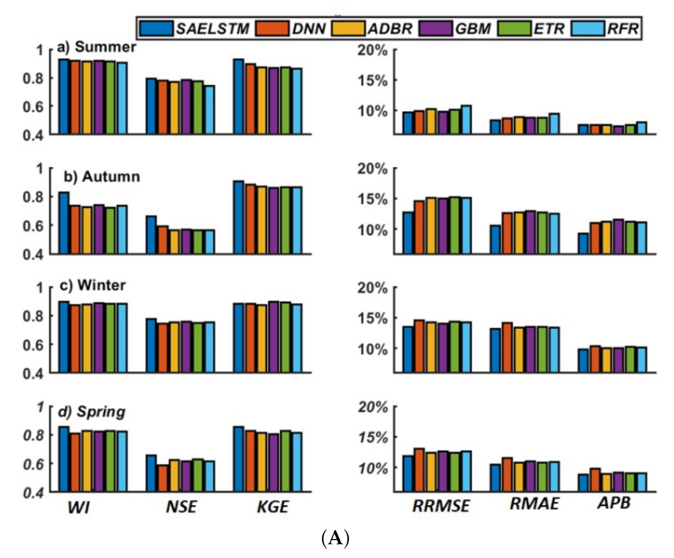
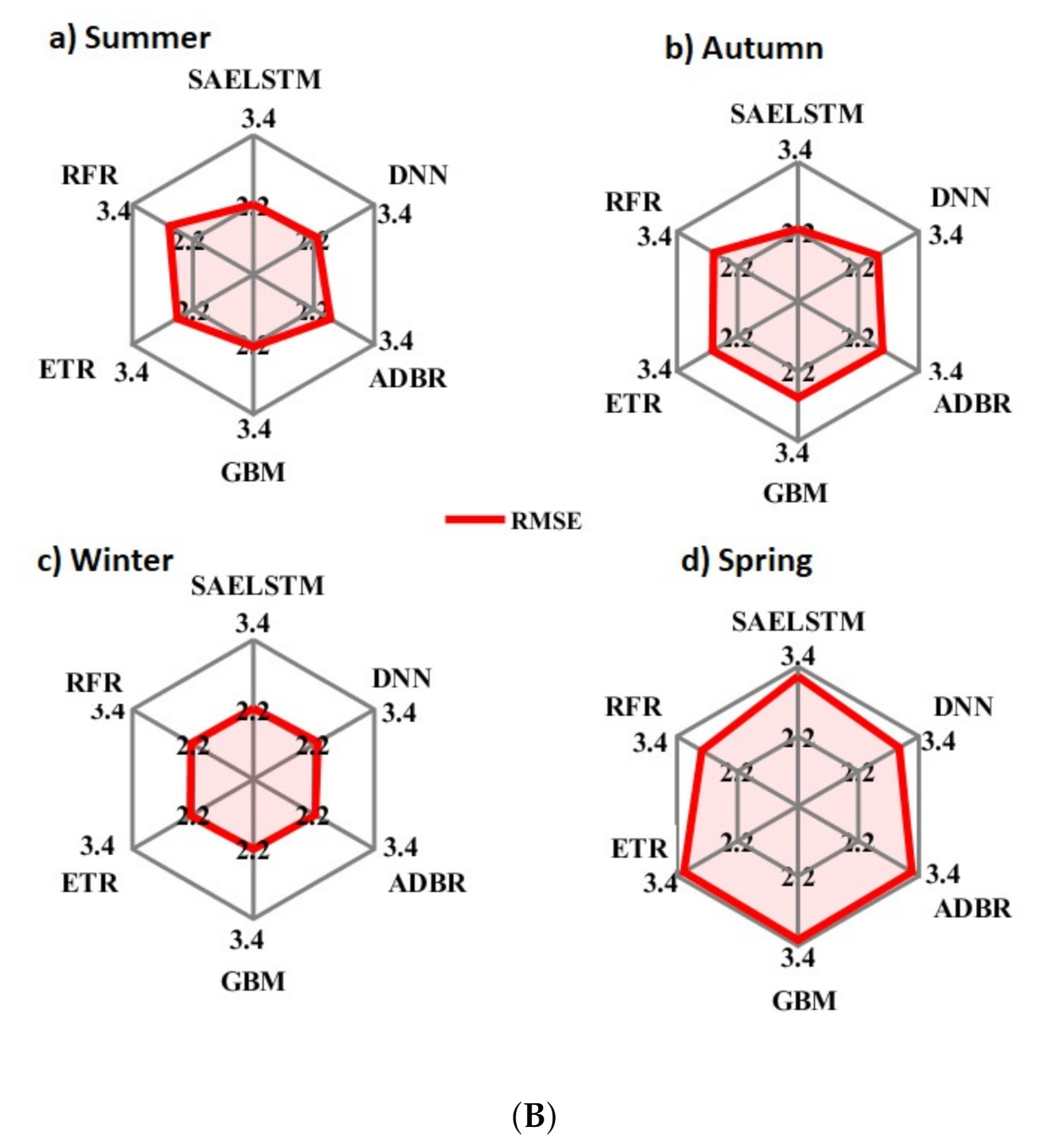
5. Results and Discussion

An extensive evaluation of the proposed deep hybrid SAELSTM model compared with the DL model (DNN) as well as the conventional ML models (GBM, RFR, ETR, and ADBR) has been conducted after the prediction of GSR at six solar farms located in Queensland, Australia. To achieve optimal features for the predictor variables, the Manta Ray Foraging Optimization (MRFO) feature selection algorithm was incorporated. In order to find the optimal hyperparameter for deep hybrid SAELSTM as well as comparative models, a grid search method based on five-fold cross-validation was used. Based on predictor metrices (Section 4.3 and Section 4.4) and visual plots, the models were assessed based on prediction results using the testing dataset. The model that showed the lowest RMSE, MSE, RRMSE, RMAE, MAPE, and APB values and the highest KGE, NSE, r, LM, and WI was chosen, and finally, the models were ranked on the basis of GPI.

In terms of statistical metrics r, RMSE, and MAE,

Table 4. The performance of the proposed deep learning hybrid SAELSTM vs. counterpart comparison models in terms of correlation coefficient (r) and root mean square error (RMSE, MJm${}^{-2}$day${}^{-1}$) in the model’s testing phase.

Predictive Models	Blair Athol Solar Power Station		Blue Grass Solar Farm		Bluff Solar Farm		Bouldercombe Solar Farm		Broadlea Solar Farm		Columboola Solar Farm
	r	RMSE	r	RMSE	r	RMSE	r	RMSE	r	RMSE	r	RMSE
SAELSTM	0.956	2.344	0.965	2.340	0.954	2.503	0.951	2.502	0.959	2.208	0.962	2.407
DNN	0.952	2.715	0.959	2.644	0.946	2.696	0.946	2.555	0.954	2.354	0.956	2.634
ADBR	0.952	2.436	0.958	2.601	0.944	2.674	0.938	2.748	0.954	2.377	0.957	2.664
GBM	0.953	2.441	0.956	2.671	0.948	2.580	0.945	2.620	0.957	2.295	0.953	2.759
ETR	0.953	2.445	0.959	2.592	0.947	2.619	0.939	2.733	0.953	2.426	0.955	2.716
RFR	0.952	2.456	0.955	2.660	0.940	2.760	0.939	2.724	0.952	2.420	0.953	2.744

and Figure 7 analyze the robustness of the deep hybrid SAELSTM against the comparison DL model and traditional ML models. In predicting GSR using all six solar farms, the proposed (deep hybrid SAESTM) model outperformed the alternative models used in this study. The results recorded the highest r value from the deep hybrid SAESTM model ($0.962\le r\ge 0.954$) and the lowest RMSE and MAE values ($2.503\le$RMSE (MJm${}^{-2}$day${}^{-1}$) $\ge 2.208$ and $1.967\le$MAE (MJm${}^{-2}$day${}^{-1}$) $\ge 1.638)$ in comparison with the other models. Consequently, it was clear that the deep hybrid SAESTM model is superior to DNN and other comparing models.

In

Table 5. As per Table 5 but measured in terms of the Willmott’s Index (WI) and Nash–Sutcliffe coefficients (NSE).

Predictive Models	Blair Athol Solar Power Station		Blue Grass Solar Farm		Bluff Solar Farm		Bouldercombe Solar Farm		Broadlea Solar Farm		Columboola Solar Farm
	WI	NSE	WI	NSE	WI	NSE	WI	NSE	WI	NSE	WI	NSE
SAELSTM	0.918	0.834	0.930	0.863	0.916	0.820	0.885	0.799	0.926	0.845	0.925	0.854
DNN	0.885	0.785	0.904	0.828	0.881	0.791	0.881	0.788	0.910	0.824	0.911	0.826
ADBR	0.911	0.821	0.906	0.832	0.897	0.793	0.858	0.757	0.909	0.822	0.902	0.824
GBM	0.911	0.820	0.902	0.823	0.906	0.807	0.874	0.780	0.918	0.833	0.896	0.811
ETR	0.911	0.820	0.908	0.833	0.903	0.801	0.862	0.761	0.906	0.815	0.899	0.817
RFR	0.910	0.818	0.902	0.824	0.891	0.779	0.861	0.762	0.907	0.815	0.899	0.812

, we employed multi-scale WI and NSE criterion to analyze the performance of the deep hybrid SAELSTM model vs. the DNN, ADBR, GBM, ETR, and RFR models. For the case of Blue Grass Solar Farm, the optimum values of WI (≈0.930) and NSE (≈0.863) were produced by the SAELSTM model followed by those for an ETR (WI ≈ 0.908, NSE ≈ 0.833), the ADBR model (WI ≈ 0.906, NSE ≈ 0.82), the DNN model (WI ≈ 0.904, NSE ≈ 0.828), the GBM model (WI ≈ 0.902, NSE ≈ 0.823), and the RFR model (WI ≈ 0.902, NSE ≈ 0.824). Similarly for the other five farms, high performance was yielded by the SAELSTM model in comparison with other methods.

The performance of the SAELSTM model was further evaluated using two other metrics of LM and $E_{var}$ (

Table 6. As per Table 5 but measured in terms of the Legates and McCabes index ($LM$) and explained variance score ($E_{var}$).

Predictive Models	Blair Athol Solar Power Station		Blue Grass Solar Farm		Bluff Solar Farm		Bouldercombe Solar Farm		Broadlea Solar Farm		Columboola Solar Farm
	$LM$	$E_{var}$	$LM$	$E_{var}$	$LM$	$E_{var}$	$LM$	$E_{var}$	$LM$	$E_{var}$	$LM$	$E_{var}$
SAELSTM	0.630	0.835	0.665	0.867	0.595	0.827	0.600	0.817	0.644	0.845	0.659	0.856
DNN	0.573	0.817	0.628	0.846	0.577	0.798	0.583	0.799	0.605	0.824	0.628	0.831
ADBR	0.616	0.823	0.633	0.842	0.582	0.793	0.568	0.773	0.621	0.829	0.631	0.837
GBM	0.618	0.823	0.612	0.836	0.592	0.807	0.579	0.798	0.626	0.838	0.608	0.825
ETR	0.615	0.824	0.638	0.846	0.591	0.802	0.573	0.779	0.609	0.825	0.617	0.829
RFR	0.612	0.820	0.624	0.833	0.573	0.780	0.581	0.778	0.616	0.821	0.614	0.822

). For the Blue Grass solar farm, the SAELSTM model with high LM (≈0.665) and $E_{var}$ (≈0.867) outperformed all the other DL models and the conventional ML models. Likewise, the SAELSTM model of the other five solar farms (Blair Athol solar power station, Bluff solar farm, Bouldercombe solar farm, Broadlea solar farm, and Columboola solar farm) performed substantially better proofing than the deep hybrid SAELSTM model, indicating its superior accuracy in predicting GSR compared to the other models developed in this work.

In order to overcome the limitation of the objective metrics, diagnostic plots were used to show the ability and suitability of the deep hybrid SAELSTM model in GSR prediction. Figure 8 shows scatter plots of the observed and predicted GSR resulting from the deep hybrid SAELSTM model, the DL models, and the conventional ML models during the testing phase at all six solar farms. For better illustration, both the linear fit equation line and the Coefficient of Determination (R${}^2$) $[Range=(0,+1);Idealvalue=+1]$, which gives a measure on the adequacy of the model [139], have been included. As it can also be seen by the scatter plot, the SAELSTM model performs the best, since the scatter points are close to the $y=mx+C$ line in comparison to the other models, which are scattered farther from the $y=mx+C$ line. The scatter plot concurs with the results of r, RMSE, MAE, LM, NSE, WI, and $E_{var}$ metrices as well.

To compare the model performances in prediction of GSR at the sites that differ geographically, physically, and climatically, alternative relative metrics such as RRMSE and RMAE were used.

Table 7. As per Table 5 but measured in terms of the relative root mean square error (RRMSE, %) and relative mean absolute error (RMAE, %) in the testing phase.

Predictive Models	Blair Athol Solar Power Station		Blue Grass Solar Farm		Bluff Solar Farm		Bouldercombe Solar Farm		Broadlea Solar Farm		Columboola Solar Farm
	RRMSE	RMAE	RRMSE	RMAE	RRMSE	RMAE	RRMSE	RMAE	RRMSE	RMAE	RRMSE	RMAE
SAELSTM	11.418	10.309	11.617	10.527	12.480	11.514	12.518	11.192	10.840	9.599	11.912	10.904
DNN	13.226	12.038	13.126	11.928	13.441	13.181	12.783	11.546	11.554	10.629	13.035	11.698
ADBR	11.867	10.519	12.910	11.895	13.334	12.329	13.749	12.125	11.668	10.305	13.188	11.955
GBM	11.894	10.465	13.259	12.441	12.866	12.044	13.106	12.035	11.266	10.041	13.657	12.706
ETR	11.910	10.371	12.868	11.790	13.060	12.218	13.671	12.045	11.911	10.501	13.440	12.225
RFR	11.967	10.496	13.208	12.166	13.763	12.542	13.630	11.828	11.881	10.252	13.579	12.337

presents these statistical metrics showing that the deep hybrid SAELSTM model had the lowest RRMSE and RMAE compared to the DNN, ADBR, GBM, ETR, and RFR approaches for all six solar farms. For example, the proposed study model yielded RRMSE ≈ 11.617% compared with 13.126 for DNN, 12.910 for ADBR, 13.259 for GBM, 12.868 for ETR, and 13.208 for RFR when the Blue Grass solar farm data were used. In all six sites, the deep hybrid SAELSTM model resulted in the lowest values of both RRMSE and RMAE, and they were lower than those of the other comparative models, indicating that the SAELSTM is undoubtedly the best option.

The predictability of the deep hybrid SAELSTM model is further evaluated by comparing promoting percentages, which are presented via incremental performance ($\lambda$) of the objective model over competing approaches, where, for example, $\lambda$ = $RMA{E}_{SAELSTM}$ − $RMA{E}_{DNN}$ tests the difference in relative RMAE of the SAELSTM and DNN model. During the testing phase,

Table 8. The promoting percentage of comparison, against objective (i.e., deep learning hybrid SAELSTM) model with percentage values indicating the improvement of the objective model over the benchmark models. Note: ${\lambda }_{RMAE}$ is the promoting percentages of relative mean absolute error, ${\lambda }_{RRMSE}$ is the promoting percentages of relative root mean square error, and ${\lambda }_{APB}$ is the promoting percentages of absolute percentage bias.

SAELSTM Compared Against	Blair Athol Solar Power Station			Blue Grass Solar Farm			Bluff Solar Farm			Bouldercombe Solar Farm			Broadlea Solar Farm			Columboola Solar Farm
	${\mathit{\lambda }}_{\mathit{RMAE}}$	${\mathit{\lambda }}_{\mathit{RRMSE}}$	${\mathit{\lambda }}_{\mathit{APB}}$	${\mathit{\lambda }}_{\mathit{RMAE}}$	${\mathit{\lambda }}_{\mathit{RRMSE}}$	${\mathit{\lambda }}_{\mathit{APB}}$	${\mathit{\lambda }}_{\mathit{RMAE}}$	${\mathit{\lambda }}_{\mathit{RRMSE}}$	${\mathit{\lambda }}_{\mathit{APB}}$	${\mathit{\lambda }}_{\mathit{RMAE}}$	${\mathit{\lambda }}_{\mathit{RRMSE}}$	${\mathit{\lambda }}_{\mathit{APB}}$	${\mathit{\lambda }}_{\mathit{RMAE}}$	${\mathit{\lambda }}_{\mathit{RRMSE}}$	${\mathit{\lambda }}_{\mathit{APB}}$	${\mathit{\lambda }}_{\mathit{RMAE}}$	${\mathit{\lambda }}_{\mathit{RRMSE}}$	${\mathit{\lambda }}_{\mathit{APB}}$
DNN	13%	11%	10%	8%	4%	8%	2%	4%	3%	7%	11%	7%	9%	9%	9%	16%	16%	11%
ADBR	11%	10%	10%	7%	2%	8%	10%	8%	11%	8%	6%	6%	11%	8%	9%	4%	4%	4%
GBM	14%	16%	13%	3%	0%	4%	5%	5%	5%	4%	5%	3%	15%	15%	13%	4%	3%	4%
ETR	11%	8%	9%	5%	0%	6%	9%	7%	10%	10%	10%	8%	13%	12%	11%	4%	4%	4%
RFR	14%	12%	13%	10%	5%	12%	9%	5%	10%	10%	8%	8%	14%	13%	13%	5%	5%	5%

contains further details regarding these values, making a clear comparison study. It is evident that deep hybrid SAELSTM performs better than the DL model (DNN) and the other conventional ML models (ADBR, GBM, ETR, and RFR).

A graphical analysis of model performance is as important to numerically evaluate the proposed model. To support our early results, we show in Figure 9a the violon plot of the deep hybrid SAELSTM model in comparison with the other models developed in this pilot study utilizing boxplots of the absolute prediction error ($\left|PE\right|={\mathit{GSR}}_{\mathit{obs}-}{\mathit{GSR}}_{\mathit{pred}}$) in the testing data. As shown in the figure, the distribution above the upper adjacent values represents the outliers of the extreme |PE|, along with their upper quartile, median, and lower quartile. The distribution of the |PE| error acquired by the deep hybrid SAELSTM model for all sites exhibits a much smaller quartile relative to the DNN, GBM, ADBR, ETR, and RFR. Additionally, to better understand the model’s precision for real-world renewable energy applications, the frequency of |PE| has been shown in different error bands (Figure 9b). The histogram of |PE| within an error bracket of $\pm 1$ MJm${}^{-2}$day${}^{-1}$ revealed this frequency that resulted from $\left|PE\right|$. Concurrent with our earlier results, the most accurate prediction of daily GSR is made by the proposed deep hybrid SAELSTM model. Remarkably, it is clear that 40% of all the $\left|PE\right|$ values are reported within the smallest error bracket of $\pm 1$ MJm${}^{-2}$day${}^{-1}$, whereas that for the DNN, GBM, ADBR, ETR, and RFR models are ≈36%, 37%, 20%, 19%, and 20%, respectively. This result also concurs with the errors being distributed into larger brackets for the DNN, GBM, ADBR, ETR, and RFR models.

While this study adopted the Nash–Sutcliffe coefficient to evaluate the proposed deep hybrid SAELSTM model, the three components of the NSE of model errors (i.e., correlation, bias, ratio of variances or coefficients of variation) were also investigated in Figure 10 to further check the performance in a balanced way using Kling–Gupta efficiency (KGE). Hence, the efficacy of the SAELSTM model was further verified using KGE and the absolute percentage bias (APB). With a relatively high KGE (≈0.914) and a comparatively low APB (≈8.763), the results showed the superior performance of the deep hybrid SAELSTM predictive model, far exceeding that for the counterpart models, as illustrated Figure 10a. Furthermore, the ranking of the models is performed according to the prediction efficiency using the GPI-based metrics. In general, we note that the GPI takes the values from −0.114 to 0.726, as shown in Figure 10b. Indeed, the highest value (≈0.726) is obtained by the deep hybrid SAELSTM predictive model that further proves the capability of the proposed model to forecast daily GSR data.

To reaffirm the superior performance of the deep hybrid SAELSTM predictive model, several statistical methods by utilizing the Diebold–Mariano (DM) and the Harvey, Leybourne, and Newbold (HLN) tests were also employed where the statistical significance of all the predictive models under this study are examined. The purpose of these tests is to deduce if the deep hybrid SAELSTM predictive model is significantly more accurate than the other comparative models (

Table 9. (a) Diebold–Mariano (DM) test statistics. To interpret this, we compare the column of the table with rows. For a positive result, the model in the column would be superior and with a negative result, the model in the row is superior. (b) Harvey, Leybourne, and Newbold statistics. (c) The Skill Score Metric (SS) for the proposed Deep Learning hybrid SAELSTM, as well as other Deep Learning and comparative models. (d) The performance of the proposed Deep Learning hybrid SAELSTM model with comparative benchmark models measured by the ratio of the root mean square error (RMSE).

(a)
Predictive Model	SAELSTM	DNN	ADBR	GBM	ETR	RFR
SAELSTM		1.777	2.219	3.447	2.454	2.526
DNN			0.365	1.491	1.012	1.318
ADBR				1.874	1.175	1.740
GBM					−0.890	−0.219
ETR						0.533
(b)
Predictive Model	SAELSTM	DNN	ADBR	GBM	ETR	RFR
SAELSTM		1.862	2.324	3.611	2.570	2.646
DNN			0.383	1.562	1.060	1.381
ADBR				1.963	1.231	1.823
GBM					−0.932	−0.230
ETR						0.558
(c)
Solar Energy Farm	SAELSTM	DNN	ADBR	GBM	ETR	RFR
Blair Athol Solar Power Station	0.706	0.682	0.605	0.681	0.680	0.677
Blue Grass Solar Farm	0.730	0.666	0.655	0.648	0.668	0.651
Bluff Solar Farm	0.678	0.632	0.626	0.657	0.647	0.608
Bouldercombe Solar Farm	0.603	0.521	0.586	0.565	0.526	0.529
Broadlea Solar Farm	0.694	0.645	0.652	0.669	0.630	0.632
Columboola Solar Farm	0.715	0.651	0.659	0.625	0.637	0.630
(d)
Predictive Model	SAELSTM	DNN	ADBR	GBM	ETR	RFR
SAELSTM		1.862	2.324	3.611	2.570	2.646
DNN			0.383	1.562	1.060	1.381
ADBR				1.963	1.231	1.823
GBM					−0.932	−0.230
ETR						0.558

a,b). Notably, the models in the column of these tables are compared with the models in the rows, and if the result is positive, the model in the column would most likely outperform the model in the row. By contrast, if it is negative, then the one in the row is superior. Similar to this result, Figure 11 shows that the DS (i.e., directional prediction accuracy) of the deep hybrid SAELSTM predictive model is greater than the other five models (an average of 69.64% compared with 58.62%, 58.57%, 50.16%, 51.12%, and 48.95%, respectively, for the DNN, ADBR, GBM, ETR, and RFR models). Congruent with the previous findings and taking together the results of DM, HLN, and DS tests, we argue that the deep hybrid SAELSTM model can predict the daily GSR data more accurately than the other models. Additionally, the RMSE values of the deep hybrid SAELSTM model and the comparative counterpart models are now compared with the RMSE values of the model developed using only the clear-sky index persistence measure [140], which is denoted as the skill score (SS) and the RMSE ratio (RMSEr) [141]. Notably, all the comparative models appear to have significantly lower SS and RMSE values relative to the deep hybrid SAELSTM predictive model, as shown in Table 9c,d.

Furthermore, this study has also done the interval prediction (IP), we verify the mean width (MPIW) and coverage probability (PICP) of the interval, both of which are indicators of whether the interval is suitable. This IP will can help solar plant managers better evaluate the effectiveness and safety of the power system as well as manage risks and costs accurately. The IP evaluation metrics of deep hybrid SAELSTM as well as other comparative models for all six solar sites are shown in

Table 10. The prediction interval quality metrics on six benchmarking models (best result in bold). The best model was assessed with high prediction interval coverage probability (PICP) and low mean prediction interval width (MPIW).

Predictive Models	SAELSTM		DNN		ADBR		GBM		ETR		RFR
	PICP	MPIW	PICP	MPIW	PICP	MPIW	PICP	MPIW	PICP	MPIW	PICP	MPIW
Blair Athol Solar Power Station	92%	7.732	93%	10.134	95%	12.208	92%	10.407	92%	8.892	90%	10.088
Blue Grass Solar Farm	93%	8.680	97%	10.453	96%	13.591	93%	11.665	95%	10.378	93%	11.398
Bluff Solar Farm	90%	7.702	95%	10.791	96%	12.239	91%	10.683	91%	9.338	91%	10.436
Bouldercombe Solar Farm	95%	9.483	93%	10.685	96%	13.511	94%	11.656	93%	9.852	93%	11.250
Broadlea Solar Farm	93%	8.411	97%	9.260	95%	11.637	93%	9.815	92%	8.443	91%	9.515
Columboola Solar Farm	95%	8.500	97%	11.169	95%	14.047	94%	11.958	93%	10.111	93%	11.557

. Compared to the deep hybrid model SAELSTM (PCP ≈ 95% and MPIW ≈ 8.50), the ADBR model produced the higher PICP (97%) and higher MPIW (11.169) using the Columboola solar farm. However, if PICP exceeds the prediction interval nominal confidence (PINC = 90%), the smaller the MPIW, the more accurate the model’s prediction. Therefore, we can conclude from Table 10 that the deep hybrid SAELSTM model yielded the low MPIW compared to the other Deep Learning and conventional ML models. Obviously, the PICP values of all the models under this study are greater than PINC, but the MPIW varies drastically. For instance, in the case of Bouldercombe, the metrics (PICP <MPIW>) were 95% <9.483>, 93% <10.685>, 96% <13.511>, 94% <11.656>, 93% <9.852>, and 93% <11.250> for SAELSTM, DNN, ADBR, GBM, ETR, and RFR respectively.

Figure 12 depicts the upper bound and lower bound for the 90% prediction interval between SAELSTM and other comparative models in daily GSR prediction. Furthermore, to affirm the suitability of the deep hybrid SAELSTM model in IP, we calculate the RRMSE, RMAE, and KGE of the upper bound, lower bound, and mean of the GSR interval (Figure 13).

Figure 13 shows that the RRMSE and RMAE for the deep hybrid SAELSTM model is significantly low, whereas the KGE was high, for all lower bounds, mean, and upper bounds, indicating that the deep hybrid SAELSTM can better reflect the uncertainty of GSR.

As an additional evaluation of the deep hybrid SAELSTM predictive model, the data of all study sites are divided into four distinct seasons, and the simulations are repeated for all models.

Figure Figure 14a is a representation of the model in terms of the performance measures of WI, NSE, KGE, RRMSE, RMAE, and APB for all four seasons. Concurrent with previous deductions for daily GSR predictions, the proposed deep hybrid SAELSTM model appears to register the best seasonal performance, with a lower value of RRMSE, RMAE, and APB and a higher value of WI, NSE, and KGE compared with equivalent metrics for the DNN, ADBR, GBM, ETR, and RFR models.

The deep hybrid SAELSTM predictive model is seen to produce a lower RMSE for the spring season (≈2.120 MJm${}^{-2}$day${}^{-1}$), followed by that of Autumn (≈2.244 MJm${}^{-2}$day${}^{-1}$), Summer (≈2.408 MJm${}^{-2}$day${}^{-1}$), and Winter (≈2.733 MJm${}^{-2}$day${}^{-1}$), as shown in Figure Figure 14b. In accordance with this finding, we contend that the deep hybrid SAELSTM predictive model is deemed suitable for both daily and seasonal GSR predictions.

6. Conclusions, Limitations, and Future Research Directions

The goal of this study has been to develop an end-to-end method of predicting daily GSR based on a hybrid Deep Learning (DL) Stacked LSTM-based seq2seq (SAELSTM) model. For this purpose, six solar energy farms located in Queensland, Australia were selected as the study sites, and a number of predictors from Global Climate Models (GCM) meteorological data and ground-based observation data from Scientific Information for Landowners (SILO) were used. To build the proposed DL hybrid SAELSTM model, we have integrated the Manta Ray Foraging Optimization (MRFO) feature selection process to select the optimal features. Then, these optimal features are used as the input to the LSTM-based seq2seq architecture to predict the GSR. Comparisons with a different DL model (DNN) and conventional ML-based models (GBM, ADBR, ETR, and RFR) have been carried out.

The simulation results obtained have revealed that the accuracy of the deep hybrid SAELSTM model is substantially better than comparative models, and they confirm that the deep hybrid learning models can accurately predict GSR. In addition, prediction intervals were constructed using quantile regression to quantify the uncertainty in model parameters. The quality of predictive indicators generated by the proposed deep hybrid SAELSTM model as well as comparative models are evaluated using PICP and MPIW performance indices. Comparing the proposed deep hybrid SAELSTM model to other DL as well as conventional ML models, the results obtained have shown that the deep hybrid SAELSTM model is more effective and superior for obtaining quality PIs with high PICP and low MPIW. In general, the proposed SAELSTM model offers superiority and innovations over other models.

While this study has demonstrated the efficacy of the proposed stacked LSTM sequence-to-sequence autoencoder model for global solar radiation prediction problems, we admit that future research in sequence-to-sequence modeling for solar energy should aim to improve the proposed predictive model by exploring cloud image-based predictions of the direct normal irradiance or the direct horizontal irradiance that are useful components of global solar radiation in photovoltaic power systems. In the present study, we have used only a stacked LSTM-based seq2seq model, but to improve the overall system, other kinds of deep learning models, such as the deep net, active learning, and transformer-based models can be tested in future studies so that real-time cloud cover (or rather total sky) images can be utilized to predict solar energy generation at solar farms and solar rooftop systems to assist solar-rich nations to reach their cleaner energy targets. The stacked LSTM-based seq2seq model can also be integrated with wavelet-based or ensemble mode decomposition approaches (e.g., Refs. [27,53,54] that have been shown to perform exceptionally well relative to the non-wavelet model. We have not yet investigated the specific effects of aerosols, atmospheric dust, ozone, and water vapor—all of which subtly affect the direct normal irradiance and the global horizontal irradiance. Considering that these effects are paramount in solar energy monitoring systems and especially relevant for behind-the-meter solar generation estimation, future research could also consider the utility of the stacked LSTM-based seq2seq model to include these exogenous effects on solar energy prediction. Advanced predictive frameworks such as deep reinforcement learning in situations where standard deep learning fails could also be developed in future research. In the renewable and sustainable energy sector, a deep hybrid based GSR predictive model can also contribute to strategic decisions (such as smart grid integration of solar energy into real-time energy management systems), as well as enabling governments and investors to make more informed decisions in the future planning of solar energy system installations. The present modeling strategies, improved through novel methods such as reinforcement learning, deep net, active learning, and transformer-based models to directly incorporate sky images in a PV system power monitoring system, can be used for applications such as physical modeling of wind and wave energy utilization and climate change scenarios with artificial intelligence models providing quality predictions.

References

1. Gielen, D.; Boshell, F.; Saygin, D.; Bazilian, M.D.; Wagner, N.; Gorini, R. The role of renewable energy in the global energy transformation. Energy Strategy Rev. 2019, 24, 38–50. [Google Scholar] [CrossRef]
2. Gielen, D.; Gorini, R.; Wagner, N.; Leme, R.; Gutierrez, L.; Prakash, G.; Asmelash, E.; Janeiro, L.; Gallina, G.; Vale, G.; et al. Global Energy Transformation: A Roadmap to 2050; Hydrogen Knowledge Centre: Derby, UK, 2019; Available online: https://www.h2knowledgecentre.com/content/researchpaper1605 (accessed on 1 December 2021).
3. Farivar, G.; Asaei, B. A new approach for solar module temperature estimation using the simple diode model. IEEE Trans. Energy Convers. 2011, 26, 1118–1126. [Google Scholar] [CrossRef]
4. Pazikadin, A.R.; Rifai, D.; Ali, K.; Malik, M.Z.; Abdalla, A.N.; Faraj, M.A. Solar irradiance measurement instrumentation and power solar generation forecasting based on Artificial Neural Networks (ANN): A review of five years research trend. Sci. Total Environ. 2020, 715, 136848. [Google Scholar] [CrossRef]
5. Amiri, B.; Gómez-Orellana, A.M.; Gutiérrez, P.A.; Dizène, R.; Hervás-Martínez, C.; Dahmani, K. A novel approach for global solar irradiation forecasting on tilted plane using Hybrid Evolutionary Neural Networks. J. Clean. Prod. 2021, 287, 125577. [Google Scholar] [CrossRef]
6. Yang, K.; Koike, T.; Ye, B. Improving estimation of hourly, daily, and monthly solar radiation by importing global data sets. Agric. For. Meteorol. 2006, 137, 43–55. [Google Scholar] [CrossRef]
7. Salcedo-Sanz, S.; Ghamisi, P.; Piles, M.; Werner, M.; Cuadra, L.; Moreno-Martínez, A.; Izquierdo-Verdiguier, E.; Muñoz-Marí, J.; Mosavi, A.; Camps-Valls, G. Machine learning information fusion in Earth observation: A comprehensive review of methods, applications and data sources. Inf. Fusion 2020, 63, 256–272. [Google Scholar] [CrossRef]
8. García-Hinde, O.; Terrén-Serrano, G.; Hombrados-Herrera, M.; Gómez-Verdejo, V.; Jiménez-Fernández, S.; Casanova-Mateo, C.; Sanz-Justo, J.; Martínez-Ramón, M.; Salcedo-Sanz, S. Evaluation of dimensionality reduction methods applied to numerical weather models for solar radiation forecasting. Eng. Appl. Artif. Intell. 2018, 69, 157–167. [Google Scholar] [CrossRef]
9. Jiang, Y. Computation of monthly mean daily global solar radiation in China using artificial neural networks and comparison with other empirical models. Energy 2009, 34, 1276–1283. [Google Scholar] [CrossRef]
10. Al-Musaylh, M.S.; Deo, R.C.; Adamowski, J.F.; Li, Y. Short-term electricity demand forecasting with MARS, SVR and ARIMA models using aggregated demand data in Queensland, Australia. Adv. Eng. Inform. 2018, 35, 1–16. [Google Scholar] [CrossRef]
11. Huang, J.; Korolkiewicz, M.; Agrawal, M.; Boland, J. Forecasting solar radiation on an hourly time scale using a Coupled AutoRegressive and Dynamical System (CARDS) model. Sol. Energy 2013, 87, 136–149. [Google Scholar] [CrossRef]
12. Shadab, A.; Said, S.; Ahmad, S. Box–Jenkins multiplicative ARIMA modeling for prediction of solar radiation: A case study. Int. J. Energy Water Resour. 2019, 3, 305–318. [Google Scholar] [CrossRef]
13. Zang, H.; Liu, L.; Sun, L.; Cheng, L.; Wei, Z.; Sun, G. Short-term global horizontal irradiance forecasting based on a hybrid CNN-LSTM model with spatiotemporal correlations. Renew. Energy 2020, 160, 26–41. [Google Scholar] [CrossRef]
14. Mishra, S.; Palanisamy, P. Multi-time-horizon solar forecasting using recurrent neural network. In Proceedings of the 2018 IEEE Energy Conversion Congress and Exposition (ECCE), Portland, OR, USA, 23–27 September 2018; IEEE: Piscataway, NJ, USA, 2018; pp. 18–24. [Google Scholar]
15. Elminir, H.K.; Areed, F.F.; Elsayed, T.S. Estimation of solar radiation components incident on Helwan site using neural networks. Sol. Energy 2005, 79, 270–279. [Google Scholar] [CrossRef]
16. Al-Musaylh, M.S.; Deo, R.C.; Adamowski, J.F.; Li, Y. Short-term electricity demand forecasting using machine learning methods enriched with ground-based climate and ECMWF Reanalysis atmospheric predictors in southeast Queensland, Australia. Renew. Sustain. Energy Rev. 2019, 113, 109293. [Google Scholar] [CrossRef]
17. Salcedo-Sanz, S.; Deo, R.C.; Cornejo-Bueno, L.; Camacho-Gómez, C.; Ghimire, S. An efficient neuro-evolutionary hybrid modelling mechanism for the estimation of daily global solar radiation in the Sunshine State of Australia. Appl. Energy 2018, 209, 79–94. [Google Scholar] [CrossRef]
18. Guijo-Rubio, D.; Durán-Rosal, A.; Gutiérrez, P.; Gómez-Orellana, A.; Casanova-Mateo, C.; Sanz-Justo, J.; Salcedo-Sanz, S.; Hervás-Martínez, C. Evolutionary artificial neural networks for accurate solar radiation prediction. Energy 2020, 210, 118374. [Google Scholar] [CrossRef]
19. Bouzgou, H.; Gueymard, C.A. Minimum redundancy–maximum relevance with extreme learning machines for global solar radiation forecasting: Toward an optimized dimensionality reduction for solar time series. Sol. Energy 2017, 158, 595–609. [Google Scholar] [CrossRef]
20. Al-Musaylh, M.S.; Deo, R.C.; Li, Y. Electrical energy demand forecasting model development and evaluation with maximum overlap discrete wavelet transform-online sequential extreme learning machines algorithms. Energies 2020, 13, 2307. [Google Scholar] [CrossRef]
21. Salcedo-Sanz, S.; Casanova-Mateo, C.; Pastor-Sánchez, A.; Sánchez-Girón, M. Daily global solar radiation prediction based on a hybrid Coral Reefs Optimization–Extreme Learning Machine approach. Sol. Energy 2014, 105, 91–98. [Google Scholar] [CrossRef]
22. Aybar-Ruiz, A.; Jiménez-Fernández, S.; Cornejo-Bueno, L.; Casanova-Mateo, C.; Sanz-Justo, J.; Salvador-González, P.; Salcedo-Sanz, S. A novel grouping genetic algorithm–extreme learning machine approach for global solar radiation prediction from numerical weather models inputs. Sol. Energy 2016, 132, 129–142. [Google Scholar] [CrossRef]
23. AlKandari, M.; Ahmad, I. Solar power generation forecasting using ensemble approach based on deep learning and statistical methods. Appl. Comput. Inform. 2020. [Google Scholar] [CrossRef]
24. AL-Musaylh, M.S.; Al-Daffaie, K.; Prasad, R. Gas consumption demand forecasting with empirical wavelet transform based machine learning model: A case study. Int. J. Energy Res. 2021, 45, 15124–15138. [Google Scholar] [CrossRef]
25. Salcedo-Sanz, S.; Casanova-Mateo, C.; Muñoz-Marí, J.; Camps-Valls, G. Prediction of daily global solar irradiation using temporal Gaussian processes. IEEE Geosci. Remote Sens. Lett. 2014, 11, 1936–1940. [Google Scholar] [CrossRef]
26. Chen, J.L.; Li, G.S. Evaluation of support vector machine for estimation of solar radiation from measured meteorological variables. Theor. Appl. Climatol. 2014, 115, 627–638. [Google Scholar] [CrossRef]
27. Al-Musaylh, M.S.; Deo, R.C.; Li, Y.; Adamowski, J.F. Two-phase particle swarm optimized-support vector regression hybrid model integrated with improved empirical mode decomposition with adaptive noise for multiple-horizon electricity demand forecasting. Appl. Energy 2018, 217, 422–439. [Google Scholar] [CrossRef]
28. Al-Musaylh, M.S.; Deo, R.C.; Li, Y. Particle swarm optimized–support vector regression hybrid model for daily horizon electricity demand forecasting using climate dataset. In Proceedings of the 3rd International Conference on Power and Renewable Energy, Berlin, Germany, 21–24 September 2018; Volume 64. [Google Scholar] [CrossRef]
29. Hocaoğlu, F.O. Novel analytical hourly solar radiation models for photovoltaic based system sizing algorithms. Energy Convers. Manag. 2010, 51, 2921–2929. [Google Scholar] [CrossRef]
30. Rodríguez-Benítez, F.J.; Arbizu-Barrena, C.; Huertas-Tato, J.; Aler-Mur, R.; Galván-León, I.; Pozo-Vázquez, D. A short-term solar radiation forecasting system for the Iberian Peninsula. Part 1: Models description and performance assessment. Sol. Energy 2020, 195, 396–412. [Google Scholar] [CrossRef]
31. Linares-Rodríguez, A.; Ruiz-Arias, J.A.; Pozo-Vázquez, D.; Tovar-Pescador, J. Generation of synthetic daily global solar radiation data based on ERA-Interim reanalysis and artificial neural networks. Energy 2011, 36, 5356–5365. [Google Scholar] [CrossRef]
32. Sivamadhavi, V.; Selvaraj, R.S. Prediction of monthly mean daily global solar radiation using Artificial Neural Network. J. Earth Syst. Sci. 2012, 121, 1501–1510. [Google Scholar] [CrossRef] [Green Version]
33. Khodayar, M.; Kaynak, O.; Khodayar, M.E. Rough deep neural architecture for short-term wind speed forecasting. IEEE Trans. Ind. Informatics 2017, 13, 2770–2779. [Google Scholar] [CrossRef]
34. Bengio, Y. Learning Deep Architectures for AI; Now Publishers Inc.: Delft, The Netherlands, 2009; Available online: https://books.google.es/books?hl=es&lr=&id=cq5ewg7FniMC&oi=fnd&pg=PA1&dq=Learning+Deep+Architectures+for+AI%7D%3B+%5Chl%7BNow+Publishers+Inc.:city,+country&ots=Kpi7OXklKw&sig=JHafuLqX_O0_PsqA7BaPLFOY_zg&redir_esc=y#v=onepage&q&f=false (accessed on 1 December 2021).
35. Sun, S.; Chen, W.; Wang, L.; Liu, X.; Liu, T.Y. On the depth of deep neural networks: A theoretical view. In Proceedings of the AAAI Conference on Artificial Intelligence, Phoenix, AZ, USA, 12–17 February 2016; Volume 30. [Google Scholar]
36. Wang, F.; Zhang, Z.; Liu, C.; Yu, Y.; Pang, S.; Duić, N.; Shafie-Khah, M.; Catalão, J.P. Generative adversarial networks and convolutional neural networks based weather classification model for day ahead short-term photovoltaic power forecasting. Energy Convers. Manag. 2019, 181, 443–462. [Google Scholar] [CrossRef]
37. Kawaguchi, K.; Kaelbling, L.P.; Bengio, Y. Generalization in deep learning. arXiv 2017, arXiv:1710.05468. [Google Scholar]
38. Khodayar, M.; Wang, J. Spatio-temporal graph deep neural network for short-term wind speed forecasting. IEEE Trans. Sustain. Energy 2018, 10, 670–681. [Google Scholar] [CrossRef]
39. Ziyabari, S.; Du, L.; Biswas, S. Short-term Solar Irradiance Forecasting Based on Multi-Branch Residual Network. In Proceedings of the 2020 IEEE Energy Conversion Congress and Exposition (ECCE), Detroit, MI, USA, 11–15 October 2020; IEEE: Piscataway, NJ, USA, 2020; pp. 2000–2005. [Google Scholar]
40. Abdel-Nasser, M.; Mahmoud, K.; Lehtonen, M. Reliable solar irradiance forecasting approach based on choquet integral and deep LSTMs. IEEE Trans. Ind. Informatics 2020, 17, 1873–1881. [Google Scholar] [CrossRef]
41. Huang, X.; Zhang, C.; Li, Q.; Tai, Y.; Gao, B.; Shi, J. A comparison of hour-ahead solar irradiance forecasting models based on LSTM network. Math. Probl. Eng. 2020, 2020, 4251517. [Google Scholar] [CrossRef]
42. Gao, B.; Huang, X.; Shi, J.; Tai, Y.; Zhang, J. Hourly forecasting of solar irradiance based on CEEMDAN and multi-strategy CNN-LSTM neural networks. Renew. Energy 2020, 162, 1665–1683. [Google Scholar] [CrossRef]
43. Kumari, P.; Toshniwal, D. Long short term memory–convolutional neural network based deep hybrid approach for solar irradiance forecasting. Appl. Energy 2021, 295, 117061. [Google Scholar] [CrossRef]
44. Ziyabari, S.; Du, L.; Biswas, S. A Spatio-temporal Hybrid Deep Learning Architecture for Short-term Solar Irradiance Forecasting. In Proceedings of the 2020 47th IEEE Photovoltaic Specialists Conference (PVSC), Calgary, ON, Canada, 15 June–21 August 2020; IEEE: Piscataway, NJ, USA, 2020; pp. 0833–0838. [Google Scholar]
45. Srivastava, S.; Lessmann, S. A comparative study of LSTM neural networks in forecasting day-ahead global horizontal irradiance with satellite data. Solar Energy 2018, 162, 232–247. [Google Scholar] [CrossRef]
46. Aslam, M.; Lee, J.M.; Kim, H.S.; Lee, S.J.; Hong, S. Deep learning models for long-term solar radiation forecasting considering microgrid installation: A comparative study. Energies 2020, 13, 147. [Google Scholar] [CrossRef] [Green Version]
47. Brahma, B.; Wadhvani, R. Solar irradiance forecasting based on deep learning methodologies and multi-site data. Symmetry 2020, 12, 1830. [Google Scholar] [CrossRef]
48. Liu, F.; Zhou, X.; Cao, J.; Wang, Z.; Wang, T.; Wang, H.; Zhang, Y. Anomaly detection in quasi-periodic time series based on automatic data segmentation and attentional lstm-cnn. IEEE Trans. Knowl. Data Eng. 2020. [Google Scholar] [CrossRef]
49. Li, J.Y.; Zhan, Z.H.; Wang, H.; Zhang, J. Data-driven evolutionary algorithm with perturbation-based ensemble surrogates. IEEE Trans. Cybern. 2020, 51, 3925–3937. [Google Scholar] [CrossRef] [PubMed]
50. Bendali, W.; Saber, I.; Bourachdi, B.; Boussetta, M.; Mourad, Y. Deep learning using genetic algorithm optimization for short term solar irradiance forecasting. In Proceedings of the 2020 Fourth International Conference On Intelligent Computing in Data Sciences (ICDS), Fez, Morocco, 21–23 October 2020; IEEE: Piscataway, NJ, USA, 2020; pp. 1–8. [Google Scholar]
51. Ghimire, S.; Deo, R.C.; Raj, N.; Mi, J. Deep solar radiation forecasting with convolutional neural network and long short-term memory network algorithms. Appl. Energy 2019, 253, 113541. [Google Scholar] [CrossRef]
52. Husein, M.; Chung, I.Y. Day-ahead solar irradiance forecasting for microgrids using a long short-term memory recurrent neural network: A deep learning approach. Energies 2019, 12, 1856. [Google Scholar] [CrossRef] [Green Version]
53. Deo, R.C.; Wen, X.; Qi, F. A wavelet-coupled support vector machine model for forecasting global incident solar radiation using limited meteorological dataset. Appl. Energy 2016, 168, 568–593. [Google Scholar] [CrossRef]
54. Ghimire, S.; Deo, R.C.; Raj, N.; Mi, J. Wavelet-based 3-phase hybrid SVR model trained with satellite-derived predictors, particle swarm optimization and maximum overlap discrete wavelet transform for solar radiation prediction. Renew. Sustain. Energy Rev. 2019, 113, 109247. [Google Scholar] [CrossRef]
55. Attoue, N.; Shahrour, I.; Younes, R. Smart building: Use of the artificial neural network approach for indoor temperature forecasting. Energies 2018, 11, 395. [Google Scholar] [CrossRef] [Green Version]
56. Bandara, K.; Shi, P.; Bergmeir, C.; Hewamalage, H.; Tran, Q.; Seaman, B. Sales demand forecast in e-commerce using a long short-term memory neural network methodology. In Proceedings of the International Conference on Neural Information Processing, Sydney, NSW, Australia, 12–15 December 2019; Springer: Berlin/Heidelberg, Germany, 2019; pp. 462–474. [Google Scholar]
57. Zhao, W.; Zhang, Z.; Wang, L. Manta ray foraging optimization: An effective bio-inspired optimizer for engineering applications. Eng. Appl. Artif. Intell. 2020, 87, 103300. [Google Scholar] [CrossRef]
58. Shaheen, A.M.; Ginidi, A.R.; El-Sehiemy, R.A.; Ghoneim, S.S. Economic power and heat dispatch in cogeneration energy systems using manta ray foraging optimizer. IEEE Access 2020, 8, 208281–208295. [Google Scholar] [CrossRef]
59. Elattar, E.E.; Shaheen, A.M.; El-Sayed, A.M.; El-Sehiemy, R.A.; Ginidi, A.R. Optimal operation of automated distribution networks based-MRFO algorithm. IEEE Access 2021, 9, 19586–19601. [Google Scholar] [CrossRef]
60. Turgut, O.E. A novel chaotic manta-ray foraging optimization algorithm for thermo-economic design optimization of an air-fin cooler. SN Appl. Sci. 2021, 3, 1–36. [Google Scholar] [CrossRef]
61. Sheng, B.; Pan, T.; Luo, Y.; Jermsittiparsert, K. System Identification of the PEMFCs based on Balanced Manta-Ray Foraging Optimization algorithm. Energy Rep. 2020, 6, 2887–2896. [Google Scholar] [CrossRef]
62. Qing, X.; Niu, Y. Hourly day-ahead solar irradiance prediction using weather forecasts by LSTM. Energy 2018, 148, 461–468. [Google Scholar] [CrossRef]
63. Wang, J.Q.; Du, Y.; Wang, J. LSTM based long-term energy consumption prediction with periodicity. Energy 2020, 197, 117197. [Google Scholar] [CrossRef]
64. Zhou, C.; Chen, X. Predicting China’s energy consumption: Combining machine learning with three-layer decomposition approach. Energy Rep. 2021, 7, 5086–5099. [Google Scholar] [CrossRef]
65. Gers, F.A.; Schmidhuber, J.; Cummins, F. Learning to forget: Continual prediction with LSTM. Neural Comput. 2000, 12, 2451–2471. [Google Scholar] [CrossRef] [PubMed]
66. Cho, K.; Van Merriënboer, B.; Gulcehre, C.; Bahdanau, D.; Bougares, F.; Schwenk, H.; Bengio, Y. Learning phrase representations using RNN encoder-decoder for statistical machine translation. arXiv 2014, arXiv:1406.1078. [Google Scholar]
67. Jang, M.; Seo, S.; Kang, P. Recurrent neural network-based semantic variational autoencoder for sequence-to-sequence learning. Inf. Sci. 2019, 490, 59–73. [Google Scholar] [CrossRef] [Green Version]
68. He, X.; Haffari, G.; Norouzi, M. Sequence to sequence mixture model for diverse machine translation. arXiv 2018, arXiv:1810.07391. [Google Scholar]
69. Huang, J.; Sun, Y.; Zhang, W.; Wang, H.; Liu, T. Entity Highlight Generation as Statistical and Neural Machine Translation. IEEE/ACM Trans. Audio Speech Lang. Process. 2018, 26, 1860–1872. [Google Scholar] [CrossRef]
70. Hwang, S.; Jeon, G.; Jeong, J.; Lee, J. A novel time series based Seq2Seq model for temperature prediction in firing furnace process. Procedia Comput. Sci. 2019, 155, 19–26. [Google Scholar] [CrossRef]
71. Golovko, V.; Kroshchanka, A.; Mikhno, E. Deep Neural Networks: Selected Aspects of Learning and Application. Pattern Recognit. Image Anal. 2021, 31, 132–143. [Google Scholar] [CrossRef]
72. Mert, İ. Agnostic deep neural network approach to the estimation of hydrogen production for solar-powered systems. Int. J. Hydrog. Energy 2021, 46, 6272–6285. [Google Scholar] [CrossRef]
73. Jallal, M.A.; Chabaa, S.; Zeroual, A. A novel deep neural network based on randomly occurring distributed delayed PSO algorithm for monitoring the energy produced by four dual-axis solar trackers. Renew. Energy 2020, 149, 1182–1196. [Google Scholar] [CrossRef]
74. Pustokhina, I.V.; Pustokhin, D.A.; Gupta, D.; Khanna, A.; Shankar, K.; Nguyen, G.N. An effective training scheme for deep neural network in edge computing enabled Internet of medical things (IoMT) systems. IEEE Access 2020, 8, 107112–107123. [Google Scholar] [CrossRef]
75. Srinidhi, C.L.; Ciga, O.; Martel, A.L. Deep neural network models for computational histopathology: A survey. Med Image Anal. 2021, 67, 101813. [Google Scholar] [CrossRef] [PubMed]
76. Khan, A.I.; Shah, J.L.; Bhat, M.M. CoroNet: A deep neural network for detection and diagnosis of COVID-19 from chest x-ray images. Comput. Methods Programs Biomed. 2020, 196, 105581. [Google Scholar] [CrossRef]
77. Bau, D.; Zhu, J.Y.; Strobelt, H.; Lapedriza, A.; Zhou, B.; Torralba, A. Understanding the role of individual units in a deep neural network. Proc. Natl. Acad. Sci. USA 2020, 117, 30071–30078. [Google Scholar] [CrossRef]
78. Wang, F.K.; Mamo, T. Gradient boosted regression model for the degradation analysis of prismatic cells. Comput. Ind. Eng. 2020, 144, 106494. [Google Scholar] [CrossRef]
79. Breiman, L. Random forests. Mach. Learn. 2001, 45, 5–32. [Google Scholar] [CrossRef] [Green Version]
80. Friedman, J.H. Stochastic gradient boosting. Comput. Stat. Data Anal. 2002, 38, 367–378. [Google Scholar] [CrossRef]
81. Ridgeway, G. Generalized Boosted Models: A guide to the gbm package. Update 2007, 1, 2007. [Google Scholar]
82. Grape, S.; Branger, E.; Elter, Z.; Balkeståhl, L.P. Determination of spent nuclear fuel parameters using modelled signatures from non-destructive assay and Random Forest regression. Nucl. Instruments Methods Phys. Res. Sect. A Accel. Spectrometers Detect. Assoc. Equip. 2020, 969, 163979. [Google Scholar] [CrossRef]
83. Desai, S.; Ouarda, T.B. Regional hydrological frequency analysis at ungauged sites with random forest regression. J. Hydrol. 2021, 594, 125861. [Google Scholar] [CrossRef]
84. Hariharan, R. Random forest regression analysis on combined role of meteorological indicators in disease dissemination in an Indian city: A case study of New Delhi. Urban Clim. 2021, 36, 100780. [Google Scholar] [CrossRef] [PubMed]
85. Wang, F.; Wang, Y.; Zhang, K.; Hu, M.; Weng, Q.; Zhang, H. Spatial heterogeneity modeling of water quality based on random forest regression and model interpretation. Environ. Res. 2021, 202, 111660. [Google Scholar] [CrossRef] [PubMed]
86. Sahani, N.; Ghosh, T. GIS-based spatial prediction of recreational trail susceptibility in protected area of Sikkim Himalaya using logistic regression, decision tree and random forest model. Ecol. Inform. 2021, 64, 101352. [Google Scholar] [CrossRef]
87. Fouedjio, F. Exact Conditioning of Regression Random Forest for Spatial Prediction. Artif. Intell. Geosci. 2020, 1, 11–23. [Google Scholar] [CrossRef]
88. Mohammed, S.; Al-Ebraheem, A.; Holb, I.J.; Alsafadi, K.; Dikkeh, M.; Pham, Q.B.; Linh, N.T.T.; Szabo, S. Soil management effects on soil water erosion and runoff in central Syria—A comparative evaluation of general linear model and random forest regression. Water 2020, 12, 2529. [Google Scholar] [CrossRef]
89. Zhang, W.; Wu, C.; Li, Y.; Wang, L.; Samui, P. Assessment of pile drivability using random forest regression and multivariate adaptive regression splines. Georisk Assess. Manag. Risk Eng. Syst. Geohazards 2021, 15, 27–40. [Google Scholar] [CrossRef]
90. Babar, B.; Luppino, L.T.; Boström, T.; Anfinsen, S.N. Random forest regression for improved mapping of solar irradiance at high latitudes. Sol. Energy 2020, 198, 81–92. [Google Scholar] [CrossRef]
91. Geurts, P.; Ernst, D.; Wehenkel, L. Extremely randomized trees. Mach. Learn. 2006, 63, 3–42. [Google Scholar] [CrossRef] [Green Version]
92. Zhu, X.; Zhang, P.; Xie, M. A Joint Long Short-Term Memory and AdaBoost regression approach with application to remaining useful life estimation. Measurement 2021, 170, 108707. [Google Scholar] [CrossRef]
93. Xia, T.; Zhuo, P.; Xiao, L.; Du, S.; Wang, D.; Xi, L. Multi-stage fault diagnosis framework for rolling bearing based on OHF Elman AdaBoost-Bagging algorithm. Neurocomputing 2021, 433, 237–251. [Google Scholar] [CrossRef]
94. Jiang, H.; Zheng, W.; Luo, L.; Dong, Y. A two-stage minimax concave penalty based method in pruned AdaBoost ensemble. Appl. Soft Comput. 2019, 83, 105674. [Google Scholar] [CrossRef]
95. Mehmood, Z.; Asghar, S. Customizing SVM as a base learner with AdaBoost ensemble to learn from multi-class problems: A hybrid approach AdaBoost-MSVM. Knowl.-Based Syst. 2021, 217, 106845. [Google Scholar] [CrossRef]
96. Xiao, C.; Chen, N.; Hu, C.; Wang, K.; Gong, J.; Chen, Z. Short and mid-term sea surface temperature prediction using time-series satellite data and LSTM-AdaBoost combination approach. Remote Sens. Environ. 2019, 233, 111358. [Google Scholar] [CrossRef]
97. CEC. Clean Energy Australia Report; CEC: Melbourne, Australia, 2020. [Google Scholar]
98. CEC. Clean Energy Australia Report 2021; CEC: Melbourne, Australia, 2021. [Google Scholar]
99. List of Solar Farms in Queensland—Wikipedia. 2021. Available online: https://en.wikipedia.org/wiki/List_of_solar_farms_in_Queensland (accessed on 1 December 2021).
100. Stone, G.; Dalla Pozza, R.; Carter, J.; McKeon, G. Long Paddock: Climate risk and grazing information for Australian rangelands and grazing communities. Rangel. J. 2019, 41, 225–232. [Google Scholar] [CrossRef]
101. Centre for Environmental Data Analysis. CEDA Archive; Centre for Environmental Data Analysis: Leeds, UK, 2020; Available online: https://www.ceda.ac.uk/ (accessed on 1 December 2021).
102. The Commonwealth Scientific and Industrial Research Organisation; Bureau of Meteorology. WCRP CMIP5: The CSIRO-BOM team ACCESS1-0 Model Output Collection; Centre for Environmental Data Analysis: Leeds, UK, 2017; Available online: https://www.csiro.au/ (accessed on 1 December 2021).
103. Met Office Hadley Centre. WCRP CMIP5: Met Office Hadley Centre (MOHC) HadGEM2-CC Model Output Collection; Centre for Environmental Data Analysis: Leeds, UK, 2012; Available online: https://catalogue.ceda.ac.uk/uuid/2e4f5b3748874c61a265f58039898ea5 (accessed on 1 December 2021).
104. Meteorological Research Institute of the Korean Meteorological Administration WCRP CMIP5: Meteorological Research Institute of KMA MRI-CGCM3 Model Output Collection; Centre for Environmental Data Analysis: Oxon, UK. 2013. Available online: https://data-search.nerc.ac.uk/geonetwork/srv/api/records/d8fefd3b748541e69e69154c7933eba1 (accessed on 1 December 2021).
105. Ghimire, S.; Deo, R.C.; Downs, N.J.; Raj, N. Global solar radiation prediction by ANN integrated with European Centre for medium range weather forecast fields in solar rich cities of Queensland Australia. J. Clean. Prod. 2019, 216, 288–310. [Google Scholar] [CrossRef]
106. Ghimire, S.; Deo, R.C.; Downs, N.J.; Raj, N. Self-adaptive differential evolutionary extreme learning machines for long-term solar radiation prediction with remotely-sensed MODIS satellite and Reanalysis atmospheric products in solar-rich cities. Remote Sens. Environ. 2018, 212, 176–198. [Google Scholar] [CrossRef]
107. Ghimire, S.; Yaseen, Z.M.; Farooque, A.A.; Deo, R.C.; Zhang, J.; Tao, X. Streamflow prediction using an integrated methodology based on convolutional neural network and long short-term memory networks. Sci. Rep. 2021, 11, 1–26. [Google Scholar]
108. Gong, G.; An, X.; Mahato, N.K.; Sun, S.; Chen, S.; Wen, Y. Research on short-term load prediction based on Seq2seq model. Energies 2019, 12, 3199. [Google Scholar] [CrossRef] [Green Version]
109. Cavalli, S.; Amoretti, M. CNN-based multivariate data analysis for bitcoin trend prediction. Appl. Soft Comput. 2021, 101, 107065. [Google Scholar] [CrossRef]
110. Kingma, D.P.; Ba, J. Adam: A method for stochastic optimization. arXiv 2014, arXiv:1412.6980. [Google Scholar]
111. Prechelt, L. Early stopping-but when? In Neural Networks: Tricks of the Trade; Springer: Berlin/Heidelberg, Germany, 1998; pp. 55–69. [Google Scholar]
112. Chollet, F. Keras. 2017. Available online: https://keras.io/ (accessed on 1 December 2021).
113. Brownlee, J. Time series prediction with lstm recurrent neural networks in python with keras. Mach. Learn. Mastery. 2016. Available online: https://machinelearningmastery.com/time-series-prediction-lstm-recurrent-neural-networks-python-keras/ (accessed on 1 December 2021).
114. Goldsborough, P. A tour of tensorflow. arXiv 2016, arXiv:1610.01178. [Google Scholar]
115. Abadi, M.; Barham, P.; Chen, J.; Chen, Z.; Davis, A.; Dean, J.; Devin, M.; Ghemawat, S.; Irving, G.; Isard, M.; et al. Tensorflow: A system for large-scale machine learning. In Proceedings of the 12th {USENIX} Symposium on Operating Systems Design and Implementation ({OSDI} 16), Savannah, GA, USA, 2–4 November 2016; pp. 265–283. Available online: https://www.usenix.org/system/files/conference/osdi16/osdi16-abadi.pdf (accessed on 1 December 2021).
116. ASCE Task Committee on Application of Artificial Neural Networks in Hydrology. Artificial neural networks in hydrology. II: Hydrologic applications. J. Hydrol. Eng. 2000, 5, 124–137. [Google Scholar] [CrossRef]
117. ASCE Task Committee on Definition of Criteria for Evaluation of Watershed Models of the Watershed Management Committee; Irrigation and Drainage Division. Criteria for evaluation of watershed models. J. Irrig. Drain. Eng. 1993, 119, 429–442. [Google Scholar] [CrossRef]
118. Dawson, C.W.; Abrahart, R.J.; See, L.M. HydroTest: A web-based toolbox of evaluation metrics for the standardised assessment of hydrological forecasts. Environ. Model. Softw. 2007, 22, 1034–1052. [Google Scholar] [CrossRef] [Green Version]
119. Legates, D.R.; McCabe, G.J., Jr. Evaluating the use of “goodness-of-fit” measures in hydrologic and hydroclimatic model validation. Water Resour. Res. 1999, 35, 233–241. [Google Scholar] [CrossRef]
120. Willmott, C.J. On the validation of models. Phys. Geogr. 1981, 2, 184–194. [Google Scholar] [CrossRef]
121. Ghimire, S.; Deo, R.C.; Raj, N.; Mi, J. Deep learning neural networks trained with MODIS satellite-derived predictors for long-term global solar radiation prediction. Energies 2019, 12, 2407. [Google Scholar] [CrossRef] [Green Version]
122. Pan, T.; Wu, S.; Dai, E.; Liu, Y. Estimating the daily global solar radiation spatial distribution from diurnal temperature ranges over the Tibetan Plateau in China. Appl. Energy 2013, 107, 384–393. [Google Scholar] [CrossRef]
123. Willmott, C.J.; Matsuura, K. Advantages of the mean absolute error (MAE) over the root mean square error (RMSE) in assessing average model performance. Clim. Res. 2005, 30, 79–82. [Google Scholar] [CrossRef]
124. Mandeville, A.; O’connell, P.; Sutcliffe, J.; Nash, J. River flow forecasting through conceptual models part III-The Ray catchment at Grendon Underwood. J. Hydrol. 1970, 11, 109–128. [Google Scholar] [CrossRef]
125. Despotovic, M.; Nedic, V.; Despotovic, D.; Cvetanovic, S. Review and statistical analysis of different global solar radiation sunshine models. Renew. Sustain. Energy Rev. 2015, 52, 1869–1880. [Google Scholar] [CrossRef]
126. Gupta, H.V.; Kling, H.; Yilmaz, K.K.; Martinez, G.F. Decomposition of the mean squared error and NSE performance criteria: Implications for improving hydrological modelling. J. Hydrol. 2009, 377, 80–91. [Google Scholar] [CrossRef] [Green Version]
127. McKenzie, J. Mean absolute percentage error and bias in economic forecasting. Econ. Lett. 2011, 113, 259–262. [Google Scholar] [CrossRef]
128. Liu, H.; Mi, X.; Li, Y. Smart deep learning based wind speed prediction model using wavelet packet decomposition, convolutional neural network and convolutional long short term memory network. Energy Convers. Manag. 2018, 166, 120–131. [Google Scholar] [CrossRef]
129. Sun, S.; Qiao, H.; Wei, Y.; Wang, S. A new dynamic integrated approach for wind speed forecasting. Appl. Energy 2017, 197, 151–162. [Google Scholar] [CrossRef]
130. Diebold, F.X.; Mariano, R.S. Comparing predictive accuracy. J. Bus. Econ. Stat. 2002, 20, 134–144. [Google Scholar] [CrossRef]
131. Costantini, M.; Pappalardo, C. Combination of Forecast Methods Using Encompassing Tests: An Algorithm-Based Procedure; Technical Report; Reihe Ökonomie/Economics Series; Institute for Advanced Studies (IHS): Vienna, Austria, 2008; Available online: https://www.econstor.eu/handle/10419/72708 (accessed on 1 December 2021).
132. Lian, C.; Zeng, Z.; Wang, X.; Yao, W.; Su, Y.; Tang, H. Landslide displacement interval prediction using lower upper bound estimation method with pre-trained random vector functional link network initialization. Neural Netw. 2020, 130, 286–296. [Google Scholar] [CrossRef] [PubMed]
133. Wang, J.Y.; Qian, Z.; Zareipour, H.; Pei, Y.; Wang, J.Y. Performance assessment of photovoltaic modules using improved threshold-based methods. Sol. Energy 2019, 190, 515–524. [Google Scholar] [CrossRef]
134. Bremnes, J.B. Probabilistic wind power forecasts using local quantile regression. Wind. Energy Int. J. Prog. Appl. Wind. Power Convers. Technol. 2004, 7, 47–54. [Google Scholar] [CrossRef]
135. Naik, J.; Bisoi, R.; Dash, P. Prediction interval forecasting of wind speed and wind power using modes decomposition based low rank multi-kernel ridge regression. Renew. Energy 2018, 129, 357–383. [Google Scholar] [CrossRef]
136. Khosravi, A.; Nahavandi, S.; Creighton, D.; Atiya, A.F. Lower upper bound estimation method for construction of neural network-based prediction intervals. IEEE Trans. Neural Netw. 2010, 22, 337–346. [Google Scholar] [CrossRef] [PubMed]
137. Deng, Y.; Shichang, D.; Shiyao, J.; Chen, Z.; Zhiyuan, X. Prognostic study of ball screws by ensemble data-driven particle filters. J. Manuf. Syst. 2020, 56, 359–372. [Google Scholar] [CrossRef]
138. Lu, J.; Ding, J. Construction of prediction intervals for carbon residual of crude oil based on deep stochastic configuration networks. Inf. Sci. 2019, 486, 119–132. [Google Scholar] [CrossRef]
139. Hora, J.; Campos, P. A review of performance criteria to validate simulation models. Expert Syst. 2015, 32, 578–595. [Google Scholar] [CrossRef]
140. Marquez, R.; Coimbra, C.F. Proposed metric for evaluation of solar forecasting models. J. Sol. Energy Eng. 2013, 135, 011016. [Google Scholar] [CrossRef] [Green Version]
141. Yang, D.; Alessandrini, S.; Antonanzas, J.; Antonanzas-Torres, F.; Badescu, V.; Beyer, H.G.; Blaga, R.; Boland, J.; Bright, J.M.; Coimbra, C.F.; et al. Verification of deterministic solar forecasts. Sol. Energy 2020, 210, 20–37. [Google Scholar] [CrossRef]
Figure 1. Schematic of LSTM with F t = forget, I t = input, O t = output gate, C t = cell memory state, and H t = hidden state vector.
Energies 15 01061 g001
Figure 2. The schematic structure of the proposed sequence-to-sequence model. (a) A basic encoder-decoder system; (b) An extended encoder-decoder system with LSTM structure.
Energies 15 01061 g002
Figure 3. The present study area showing six solar energy farms in Queensland Australia where the deep learning hybrid stacked LSTM sequence-to-sequence autoencoder (i.e., SAELSTM) model was developed to predict daily GSR.
Energies 15 01061 g003
Figure 4. Convergence curves for MRFO feature selection on the predictors for the case of Broadlea solar energy farm.
Energies 15 01061 g004
Figure 5. The stacked LSTM sequence-to-sequence autoencoder (i.e., SAELSTM) architecture used to predict GSR at six solar energy farms in Queensland, Australia. Note: Detailed description of the notations in Section 4.3.
Energies 15 01061 g005
Figure 6. Training and validation loss, or mean square error in model development phase. Early stopping callbacks are used to halt the model if no improvement in loss for a certain number of predefined epochs is evident.
Energies 15 01061 g006
Figure 7. Evaluation of the newly proposed SAELSTM hybrid predictive model with respect to the counterpart comparison models as measured by the mean absolute error (MAE, MJm 2 day 1 ) in the testing phase. (Note: names for each model are provided in Table 3 and Table 4.)
Energies 15 01061 g007
Figure 8. Scatter plots of the observed (GSR o b s ) and predicted (GSR p r e d ) daily GSR for solar farms in Queensland. (Note: the line in red is the least-squares fit line ( y = m x + c ) to the respective scatter plots where y is the predicted GSR and x is the observed GSR. Names for each model are provided in Table 3 and Table A1) stated in Appendix A. (a) Blair Athol Solar Power Station, (b) Blue Grass Solar Farm, (c) Bluff solr Farm, (d) Bouldercombe Solar Farm, (e) Broadlea Solar Farm, (f) Columboola Solar Farm.
Energies 15 01061 g008
Figure 9. (a) Violin plots of prediction error (PE) generated in the testing phase for daily GSR prediction. (b) The cumulative frequency of daily forecast error ( ± 1.0 MJm 2 day 1 ) for all tested sites. (For model names, see Table 3 and Table A1 in Appendix A).
Energies 15 01061 g009
Figure 10. (a, top) Bar plots of prediction error chart showing a comparison of the proposed SAELSTM model using APB, percentage, and KGE in the testing phase. (b, bottom) Global performance indicator (GPI) of CLC model compared with other counterpart models. (Note: Names for each model are provided in Table 3 and Table A1 in Appendix A).
Energies 15 01061 g010
Figure 11. The performance of the proposed SAELSTM model compared to other counterpart models under study in terms of directional symmetry (DS) criteria. (Note: Names for each model are provided in Table 3 and Table A1 in the Appendix A.)
Energies 15 01061 g011
Figure 12. A comparative result showing the upper bound and lower bound for the 90% prediction interval between the proposed SAELSTM and other comparative models.
Energies 15 01061 g012
Figure 13. Performance metrics comparison of the proposed SAELSTM and other comparative counterpart models for upper, lower, and mean predication in terms of RRMSE, RMAE, and KGE.
Energies 15 01061 g013
Figure 14. (A) Seasonal performance evaluation of proposed SAELSTM model compared to other artificial intelligence-based model in terms of WI, NSE, KGE, RRMSE (%), RMAE (%), and APB, (%). (a) Summer, (b) Autumn, (c) Winter, and (d) Spring. (B) Seasonal performance evaluation of proposed SAELSTM model compared to other artificial intelligence-based models in terms of RMSE. (Note: Names for each model are provided in Table 3 and Table A1 in Appendix A).
Energies 15 01061 g014aEnergies 15 01061 g014b