Abstract
The installed capacity of photovoltaic power generation occupies an increasing proportion in the power system, and its stability is greatly affected by the fluctuation of solar radiation. Accurate prediction of solar radiation is an important prerequisite for ensuring power grid security and electricity market transactions. The current mainstream solar radiation prediction method is the deep learning method, and the structure design and data selection of the deep learning method determine the prediction accuracy and speed of the network. In this paper, we propose a novel long short-term memory (LSTM) model based on the attention mechanism and genetic algorithm (AGA-LSTM). The attention mechanism is used to assign different weights to each feature, so that the model can focus more attention on the key features. Meanwhile, the structure and data selection parameters of the model are optimized through genetic algorithms, and the time series memory and processing capabilities of LSTM are used to predict the global horizontal irradiance and direct normal irradiance after 5, 10, and 15 min. The proposed AGA-LSTM model was trained and tested with two years of data from the public database Solar Radiation Research Laboratory site of the National Renewable Energy Laboratory. The experimental results show that under the three prediction scales, the prediction performance of the AGA-LSTM model is below 20%, which effectively improves the prediction accuracy compared with the continuous model and some public methods.
1. Introduction
In recent years, the demand for energy consumption has increased, followed by a series of problems such as energy shortages and environmental degradation. In this regard, as a clean and renewable energy source, solar energy has huge potential and is garnering increasing attention [1]. However, the instability of solar energy has severely restricted the large-scale development of photovoltaic power generation. Photovoltaic power generation is highly dependent on surface solar radiation, and its volatility will have a major impact on the traditional power system when it is concentrated and connected to the grid on a large scale [2]. Therefore, it is necessary to accurately predict the amount of photovoltaic power generation, which is of great significance for ensuring the stability of the power system and rationally planning the distribution of power resources [3,4]. Solar irradiance is the most important factor affecting photovoltaic power generation. Global horizontal irradiance (GHI) and direct normal irradiance (DNI) are the key factors for photovoltaic power generation and concentrating solar power generation [5]. Accurately predicting photovoltaic power generation is essentially accurately predicting solar irradiance.
The prediction methods of solar radiation mainly include physical methods based on thermodynamics and atmospheric dynamics, and machine learning methods based on data-driven methods [6]. Because the data-driven method is flexible and has low requirements for detection data, it is more widely used in actual engineering applications [7]. Based on the data-driven solar irradiance prediction method, the mapping relationship between historical data and future solar radiation predicted values is established through the analysis and processing of historical observation data to achieve the purpose of prediction [8,9,10]. Traditional forecasting methods mostly adopt regression analysis to establish forecasting models. Daut et al. [11] constructed a Simple Linear Regression (SLR) model by analyzing the relationship between the daily mean maximum and minimum surface temperature and daily mean solar radiation. Colak et al. [12] used Auto-Regressive Moving Average Model (ARMA) and Autoregressive Integrated Moving Average Model (ARIMA) to predict multi-scale solar radiation. Tirmikci et al. [13] used regression analysis to determine the coefficients of the new regression equation, and used the new regression equation to predict the diffuse solar radiation in the Sakarya area, Turkey.
However, these regression methods above ignore the complex nonlinear relationship between solar radiation and meteorological variables, which limits their prediction accuracy [14]. With the rise of machine learning technology, a variety of machine learning models have also been used to predict solar irradiance. Belaid et al. [15] used Support Vector Machine (SVM) to predict the global solar radiation on horizontal surfaces in Ghardaia, Algeria, and the results showed that the prediction and the measured data are close. Paoli et al. [16] proposed an optimized Multilayer Perceptron (MLP), which has a better prediction effect than traditional methods. A large number of experiments have proved that the machine learning models cloud improve the prediction accuracy comparing to simple regression methods.
Compared with traditional machine learning methods, deep learning methods could build more systematic models and obtain better prediction results. Qing et al. [17] used a Long Short-Term Memory (LSTM) network. Compared with the MLP network, the root mean square error (RMSE) of the algorithm’s prediction was reduced by 42.9%. However, the model structure of LSTM method is relatively complex, and the weight and bias cannot be accurately optimized. Therefore, there is still room for improvement in prediction accuracy.
The main factors affecting the prediction accuracy of artificial neural networks are the combination of input parameters, training algorithms, and structure configuration [18]. In response to the above problems, we proposed a prediction model of long short-term memory (LSTM) based on an attention mechanism (AM) and a genetic algorithm (GA). We introduced AM as a feature selection method to calculate the attention degree of different features and evaluate the influence of different variables on the predicted value of solar irradiance. In the process of model training, features with a high degree of attention are more likely to be selected. For secondary information, the network will reduce its attention or even ignore it to improve model prediction accuracy. In addition, the GA is used to perform a global search on the model parameters to obtain the optimal solution, and the optimal parameter combination is used to build the LSTM model, which integrates various meteorological variable data to predict the GHI and DNI after 5, 10, and 15 min.
The main contributions of this paper are as follows:
- Introduce the AM to determine the influence degree of different features on the target predicted value, so that the model can focus on important variables; and
- Use the GA to search for model parameters, establish the optimal model, effectively improve the prediction speed and accuracy of the model, and prevent problems such as too long training time, slow parameter update, or even gradient disappearance.
The remainder of this paper is organized as follows: Section 2 introduces related theories, including long short-term memory, attention mechanism and genetic algorithm. Section 3 describes the experimental materials and proposes a predicting method. Section 4 analyzes the experimental results and discusses the performance of the proposed model. Finally, Section 5 summarizes the research conclusions.
2. Related Theoretical Background
2.1. Long Short-Term Memory
Recurrent neural networks (RNNs) are mainly used to process time series data. As a variant of RNNs, the long- and short-term memory networks introduce a gate mechanism to control the preservation and loss of information, which can retain information for a longer period of time, and has more advantages in solving the problem of gradient explosion and gradient disappearance during long sequence training [19]. Therefore, it is more suitable for predicting solar radiation.
A neuron of LSTM has three gates, namely, the forget gate , the input gate , and the output gate . LSTM can be described by the following mathematical expressions [20]:
where represents the weight of the LSTM cell, represents the output at the previous moment, represents the input at the current moment, represents the corresponding bias, and represents the sigmoid activation function. The forget gate determines which information to discard by multiplying with the cell state at the previous moment. When the value is 1, all the information in the cell at the previous moment is retained. When the value is 0, all information is discarded. The new information is obtained by multiplying the input gate and the updated information at the current moment, which determines the current cell state together with the retained information. Finally, the output gate is multiplied by mapped by the activation function tanh to obtain the output at the current moment.
The depth of the single-layer LSTM network is shallow, resulting in relatively average network performance [21]. In some solutions, a single-layer LSTM network is often stacked to form a multi-layer LSTM. In a multi-layer network, the output of each time step of the first layer is used as the input of the second time step, and the output of the network is determined by the output of the last time step [22].
2.2. Attention Mechanism
In the process of predicting, additional features carry more information, and the performance of the model improves accordingly. However, information overload can also lead to higher model complexity and prolong training time [23]. The attention mechanism is inspired by the human visual attention mechanism, which can assign greater weight to the more effective information among the input information, reduce the attention to other information, and effectively improve the efficiency of problem solving [24], which has been widely used in various fields such as object detection [25], neural machine translation [26], and so on [27].
We use to denote the input N pieces of information. For the ith input information, the probability of being selected is calculated by the softmax function is as:
where attention distribution represents the degree of attention of the ith information in , and:
is called the attention scoring function:
where and denote the weight matrix and bias, respectively. The information processed by the attention mechanism becomes the input information with the attention value.
2.3. Genetic Algorithm
The genetic algorithm (GA) is a search strategy inspired by Darwin’s biological evolution theory to search for the optimal solution through the process of simulating biological evolution and natural selection [28], and the details of GAs could refer to [29,30]. The implementation process of the genetic algorithm could be summarized as follows:
- (1)
- Encode each individual in the population of potential solutions to the problem;
- (2)
- A set of solutions is randomly generated as the initial population, and the fitness of each individual is calculated;
- (3)
- Refer to the fitness function to obtain new individuals through selection strategies;
- (4)
- Perform crossover and mutation operations on the new individual to produce the next set of offspring, and calculate the fitness of all individuals in it; and
- (5)
- Iterate the entire process until the stop condition is met.
In this study, a genetic algorithm is used to search for model parameters, determine the optimal model structure and input window size so that the model can maximize information without affecting performance, simplify the model structure, and reduce the training time and improve prediction accuracy.
3. Materials and Methods
3.1. Data Collection
The weather data we selected came from the public database of the Solar Radiation Research Laboratory (SRRL) of the National Renewable Energy Laboratory (NREL). The SRRL is located in Golden, Colorado, USA. The total amount of solar radiation received by SRRL is large, the observation position is excellent, and there are over 75 instruments recording the weather conditions in real time.
We selected meteorological elements closely related to solar radiation in the database, including GHI, DNI, solar zenith angle, temperature, air mass, relative humidity, opaque cloud cover, wind speed, station pressure, and aerosol optical depth. The sample range covers all the daytime data of 2018 and 2019 (the solar zenith angle is less than 90°). The sampling frequency is 1 minute. In total, there are 53,1347 groups of samples for the following experiments.
In the process of predicting the GHI, in addition to the GHI, eight factors were selected to form the input of the prediction model. These eight factors are the solar zenith angle, temperature, air mass, relative humidity, opaque cloud cover, wind speed, station pressure, and aerosol optical depth.
When predicting the DNI, the eight factors above were selected as the input of the model. When predicting GHI and DNI, the principle of dividing the dataset in this paper was to randomly select 80% of the 2018 data as the training set and the remaining 20% of the 2018 data as the validation set. The full-year data of 2019 were selected as the testing set.
3.2. Data Preprocessing
In order to reduce the influence of different dimension data on the results and improve the prediction accuracy and convergence speed of the model, meteorological data acquired were first normalized. The linear normalization method was adopted. The formula is as follows:
where is the normalized data of a certain meteorological element, is the original data, and and are the maximum and minimum values of the corresponding sequence data, respectively.
3.3. AGA-LSTM Model
The traditional LSTM has excellent performance in dealing with time series problems. However, the manual selection of parameters is inefficient and prone to failure [31]. Models established by selecting parameters through manual experience often have various problems such as low prediction accuracy, slow convergence, and overfitting [32].
In order to fully mine data information and obtain excellent prediction results, we proposed the AGA-LSTM model to predict solar radiation. The AGA-LSTM model includes three parts: the AM is used to amplify key information to extract main features, LSTM is used to predict GHI and DNI, and the GA is responsible for optimizing the model. The prediction process of the AGA-LSTM model is shown in Figure 1.
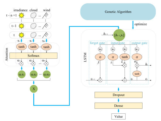
Figure 1.
The prediction process of the AGA-LSTM model.
In the predicting process, the above-mentioned eight influencing factors have different degrees of influence on the predicted value. Therefore, we introduced an attention mechanism to select the most relevant features. In the initial stage, each feature was given its own weight and bias according to the impact on the prediction result, and the corresponding score was obtained after the calculation of the tanh function. The softmax processes the scores and calculates the probability of each feature being selected, which is the attention degree. The attention degree is used to characterize the importance of the predicted value, guide the model to devote more attention to the main features, and inhibit the attention to secondary information.
When processing large quantities of data, the use of batch operations to group information with attention values can effectively speed up the calculation speed of LSTM. The input of LSTM is an n × 9 matrix, where n represents the data of the past n moments and 9 represents 9 features. The dropout layer is connected to prevent overfitting. Finally, the predicted value is output through the dense layer.
Research has found that the prediction effects of LSTMs with different structures are also quite different. Traditional methods mostly manually select parameters based on the experience of the researchers. This method not only consumes a significant amount of time, but it is also difficult to select the most suitable parameters. Therefore, we used a genetic algorithm in this study to automatically search for the optimal parameters, which significantly improves the efficiency compared to the exhaustive method.
There are many parameters of the model that need to be optimized. Among them, the number of neurons and the number of network layers determine the structure of the model, and the model structure plays a decisive role in the prediction performance. Therefore, the number of neurons and the number of network layers of the model are taken as the optimization goals of the genetic algorithm.
At the same time, the size of the input window is also related to the prediction accuracy and speed of the model. Similarly, two parameters, time step and time interval, are used when the genetic algorithm is employed to search the size of the time window.
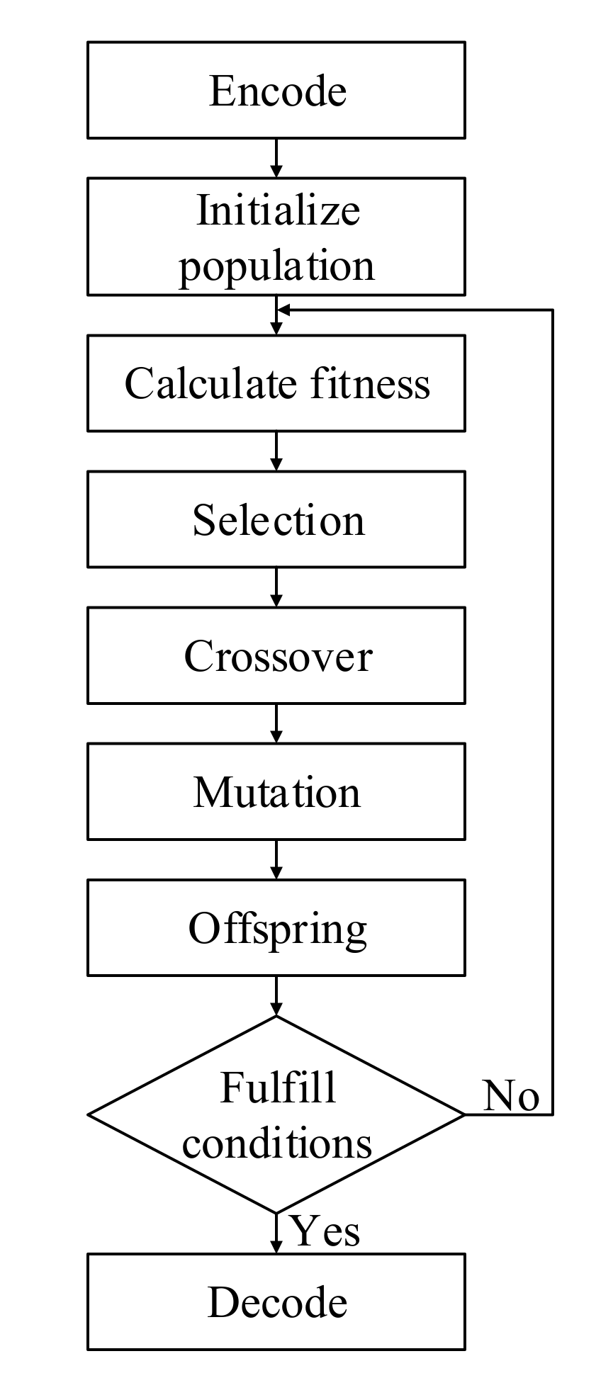
In this research, we first determined the range of 4 search parameters. According to previous research, we set the ranges for the number of neurons, the number of network layers, the time step, and the time interval as [1,16], [1,5], [1,10], and [1,10], respectively. All target parameters are integers. Therefore, each individual in the space is coded using integer coding. By initializing the population through a random number generator, calculating the fitness of each individual, new individuals were obtained scientifically through genetic operations such as selection, crossover, and mutation. Finally, an LSTM model was constructed using individual genes as parameters to predict solar radiation at a future time. The flow chart of the genetic algorithm is shown in Figure 2.
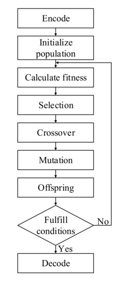
Figure 2.
The flow chart of the genetic algorithm.
Referring to the predicting errors, the fitness function of a LSTM was defined as:
where is the mean value of all data, N1 is the number of all samples, is the predicted value of the model, and is the actual value of solar irradiance.
When performing the selection operation, the roulette wheel selection strategy [33] was adopted, so that individuals or LSTMs with lower errors were selected to perform crossover and mutation with greater probability. The calculation formula for selection probability is as follows:
where represents the fitness function and represents the number of LSTM or individuals.
When applying the genetic algorithm, the parameters were set as follows: crossover rate = 0.6, mutation rate = 0.001, population size = 50, epoch = 20, iteration = 40. In other words, each individual in a population with an individual size of 50 iterates 40 times to complete one generation of iterations. A total of 40,000 iterations were completed. In the training process of the LSTM module, was used as the loss function, the Adam algorithm was used as the optimizer, and the learning rate was set to 0.1. We used the pre-divided training dataset to train the model. The optimizer continuously adjusts the parameters of the model according to the loss value generated by the training set, optimizes the model structure, and thus improves the prediction performance.
4. Results and Discussion
To evaluate the performance of the proposed method, we conducted our experiment on an Nvidia GeForce RTX 2080Ti server with Intel Core I9-9900K CPU using Python based on PyTorch’s deep learning framework.
4.1. Evaluation Index
Correlation coefficients (), normalized mean bias error (nMBE), normalized mean absolute error (nMAE), and normalized root mean squared error (nRMSE) were used to evaluate the performance of the prediction model. The calculation formulae are as follows:
where is the number of all samples, is the predicted value of the model, is the mean of all predicted values, is the measured value, and is the mean of all measured values.
In addition, the persistence model, usually used as a basis to evaluate the performance of the prediction model, is defined as:
Forecast skill () is an evaluation index defined based on the persistence model:
where and are the nRMSEs of the persistent model and the forecast model, respectively.
4.2. Performance in Predicting GHI
In this study, an attention mechanism was applied to restate the importance of different input features to the prediction model, and the model structure was optimized by a genetic algorithm. The optimization parameters included the number of LSTM cells, the number of network layers, time steps, and time intervals. The GHI prediction model was established under different prediction scales.
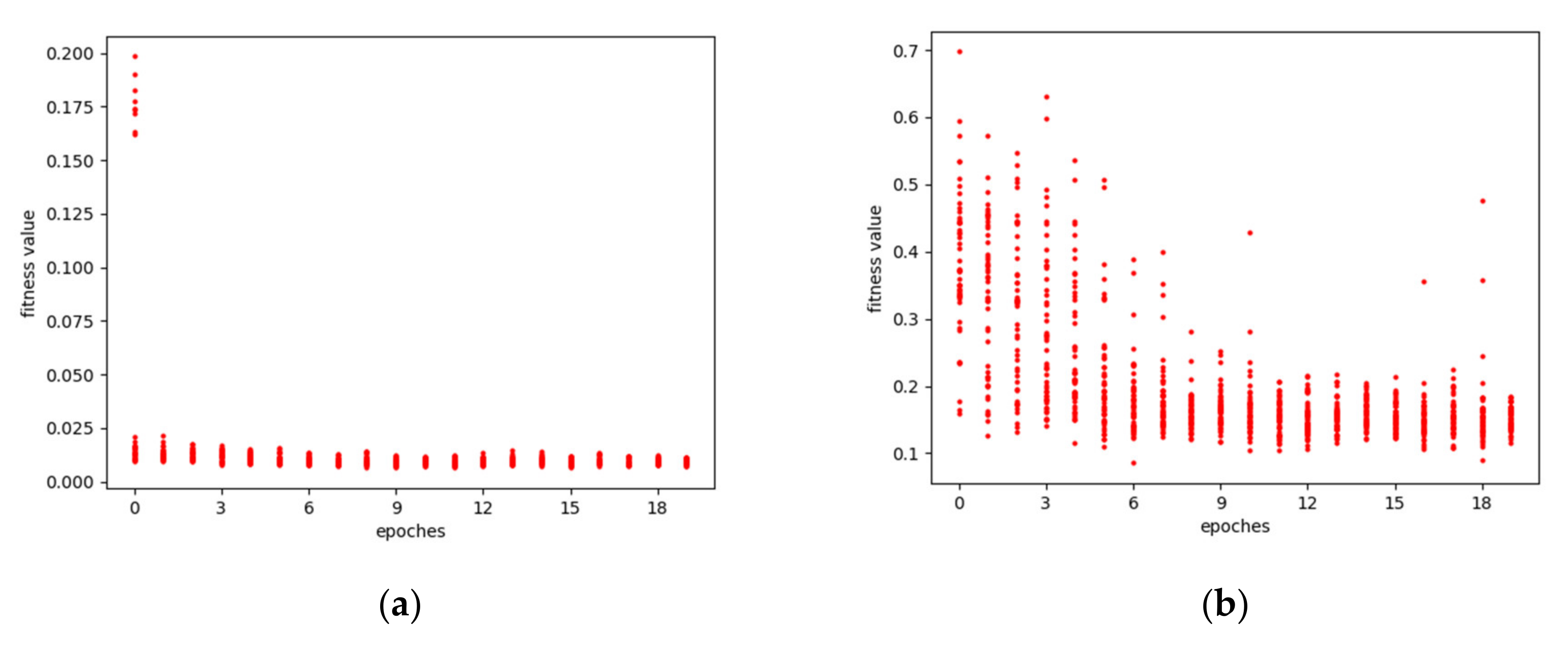
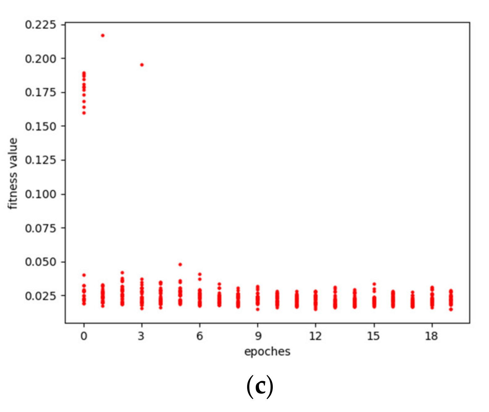
The optimization processes of the genetic algorithm for the GHI prediction model under different prediction scales is shown as Figure 3. It can be seen that in the initial stage, the fitness values, defined as Equation (6), of different individuals or LSTMs vary greatly. With the increase in the iteration number, the overall fitness value of the population tends to be consistent, although there are also few individuals that fluctuate. In the end, the fitness value of the network tends to be stable and a small value, indicating that the algorithm has reached its convergence and the predicting model has achieved greater performance, which reflects the beneficial effects of the genetic algorithm on the model.
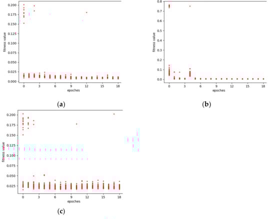
Figure 3.
The optimization processes of the GHI model: (a) 5 min prediction model optimization process; (b) 10 min prediction model optimization process; (c) 15 min prediction model optimization process.
The model was trained through the training dataset, and the final optimized parameter results of the model were obtained after testing on the validation dataset, as shown in Table 1. The number of LSTM cells represents the number of neurons in each layer of LSTM. In order to reduce optimization time and complexity, the number of neurons in each layer of a LSTM model was set the same during the optimization processes by the GA. The number of network layers represents the number of hidden layers of the LSTM network. The time step represents the dimension of the input sequence, and the time interval represents the time difference between two adjacent input sequences. Significantly, the input sequence represents the true value at certain moments, not the average value of the current time window.

Table 1.
Optimization results of the GHI prediction model parameters at different scales.
In order to evaluate the accuracy of different prediction models, the above evaluation indices were used to compare the performance of AGA-LSTM and other models. Table 2 shows the performance of the persistence models, LSTM, GA-LSTM, and AGA-LSTM under three different prediction scales. Among them, the LSTM is designed with reference [22] to the existing manual parameter selection method, and the GA-LSTM is designed without an attention mechanism. The dimensions of input variables of all models are the same.
Table 2.
The performance of AGA-LSTM models for predicting GHI.
It can be derived from Table 2 that under the three prediction scales of 5, 10, and 15 min, the nRMSEs of AGA-LSTM are 6.35%, 8.99%, and 11.28%, respectively, which are lower than other comparison models. The forecast skills of AGA-LSTM reach 83.2%, 75.8%, and 72.4% over the persistence model, respectively. These results show that AGA-LSTM has advantageous prediction performance under the prediction scale of 5, 10, and 15 min, although there is a systemic bias of the AGA-LSTM model. This is because the attention mechanism and genetic algorithm optimize the model structure, improve the learning efficiency, and work together to improve the performance of the model.
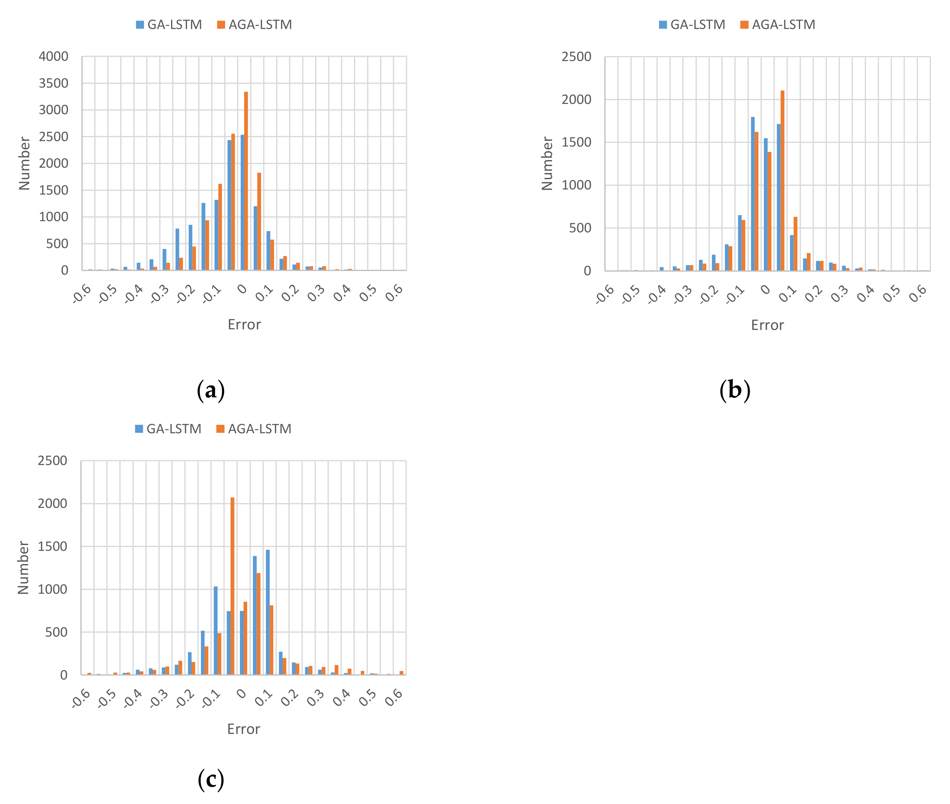
In order to further analyze the performance of the proposed model, the relative error distributions of GA-LSTM and AGA-LSTM for predicting GHI under three prediction scales were shown as Figure 4. The x-axis represents the relative error of the predicted value when the GHI was normalized as Equation (5), and the y-axis represents the number of predicted values. The more concentrated the histogram is in the range where the relative error is around 0, the better the prediction effect. It can be deduced that the error generally presents a normal distribution, and most the relative errors of the predicted value are concentrated in the range of [−0.1, 0.1], which indicates that the predicted values have a sufficient tracking effect on the real values, and AGA-LSTM can accurately predict the GHI of 5, 10, and 15 min.
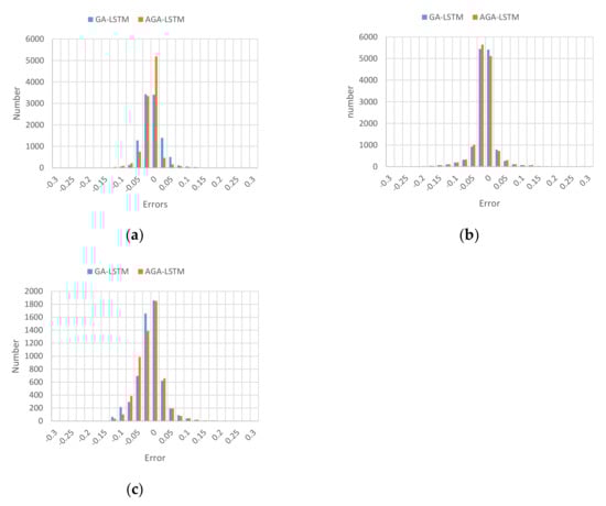
Figure 4.
The relative error distributions of GHI by GA-LSTM and AGA-LSTM; (a) error distribution of 5 min prediction model; (b) error distribution of 10 min prediction model; (c) error distribution of 15 min prediction model.
4.3. Performance in Predicting DNI
The optimization process of the genetic algorithm for DNI prediction models under different prediction scales is shown in Figure 5. Different individuals or LSTMs for predicting DNI in the initial population correspond to different fitness values that was defined as Equation (6), indicating that there are differences in the network structure constructed by different hyperparameters. As the number of iterations increases, the fitness values of different networks gradually gather, but there are also some sudden fitness values. The number of iterations continues to increase, and finally, the fitness value converges to the point that represents the best performance of the network.
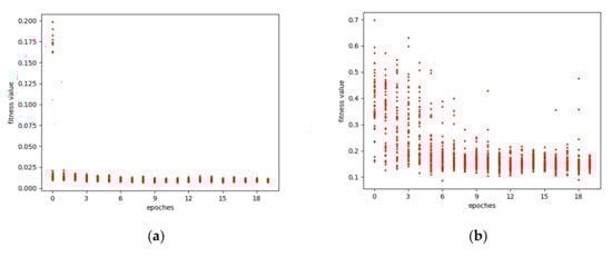
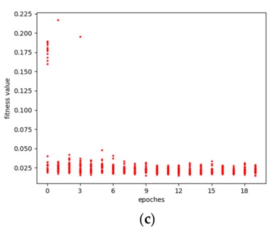
Figure 5.
The optimization processes of the DNI model; (a) 5 min prediction model optimization process; (b) 10 min prediction model optimization process; (c) 15 min prediction model optimization process.
Finally, the genetic algorithm was used to search the parameters of the DNI prediction model under different prediction scales, and the results are shown in Table 3. The number of LSTM cells, time step and time interval increased with the prediction scale when predicting DNI, which was a little different from those of the models for predicting GHI in Table 1.
Table 3.
Optimization results of DNI prediction model parameters at different scales.
In order to verify the performance of the DNI prediction model, the above evaluation indices were used to compare the performance of AGA-LSTM and other models. The results are shown in Table 4. Under the three prediction scales of 5, 10, and 15 min, the nRMSEs of AGA-LSTM are 12.68%, 11.63%, and 16.57%, respectively, which are lower than other comparison models; and the forecast skills of AGA-LSTM reach 75.9%, 77.4%, and 67.4%, respectively. This shows that at the prediction scale of 5, 10, and 15 min, AGA-LSTM has superior performance compared to other prediction models in terms of the nRMSE.
Table 4.
The performance of the AGA-LSTM model for predicting DNI.
Figure 6 shows the relative error distribution of predicting DNI under the scale of 5, 10, and 15 min when the predicting DNI was normalized as Equation (5). The relative error of most predicted values is between [−0.1, 0.1], but the number of relative errors out of the range of [−0.1, 0.1] is obviously more than that of GHI in Figure 4, which means that the prediction performance of GHI is better than that of the DNI. However, the AGA-LSTM was better than the GA-LSTM in terms of DNI prediction due to there being more errors of AGA near zero.
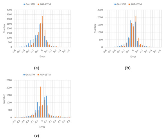
Figure 6.
The relative error distributions of DNI; (a) error distribution of 5 min prediction model; (b) error distribution of 10 min prediction model; (c) error distribution of 5 min prediction model.
5. Conclusions
In this paper, we propose an AGA-LSTM model to predict GHI and DNI at 5, 10, and 15 min time steps. LSTM is usually used to solve time series problems, but the selection of parameters restricts its performance. Our model uses attention mechanism to increase the attention of important influencing factors, and at the same time employs a genetic algorithm to search for network structure parameters and then applies them to the traditional LSTM model. The results show that the values of nRMSEs predicted by AGA-LSTM for GHI and DNI are both lower than those of other comparison models, and that the forecast skills of AGA-LSTM reach more than 67%. This shows that AGA-LSTM outperforms than other prediction models, can more effectively express complex features between data, and improve prediction accuracy and speed.
This model also has some shortcomings. The absolute values of nMBEs of the AGA-LSTM model are not the lowest, which means there is a certain systemic bias of the AGA-LSTM model. In future, we will study the influence of different meteorological factors on the prediction accuracy of the model, and select a more appropriate input combination to improve the prediction accuracy; the ground-based cloud image contains other information about the sky condition, and the model can be constructed by fusing meteorological numerical value and cloud image information to further improve the prediction performance.
Author Contributions
All authors designed this work; Conceptualization and methodology, T.Z. and Y.L.; software and validation, Z.L. and Y.G.; writing, T.Z.; visualization, T.Z. and C.N. All authors have read and agreed to the published version of the manuscript.
Funding
This research was funded by Natural Science Program of China, grant number 62006120, and the Key Laboratory of Measurement and Control of Complex Systems of Engineering (Southeast University), Ministry of Education, grant number MCCSE2020A02.
Institutional Review Board Statement
Not applicable.
Informed Consent Statement
Not applicable.
Acknowledgments
The authors acknowledge the National Renewable Energy Laboratory for providing the data used in this paper.
Conflicts of Interest
The authors declare no conflict of interest.
References
- Feng, J.; Xu, S.X. Integrated technical paradigm based novel approach towards photovoltaic power generation technology. Energy Strategy Rev. 2021, 34, 100613. [Google Scholar] [CrossRef]
- Behera, M.K.; Majumder, I.; Nayak, N. Solar photovoltaic power forecasting using optimized modified extreme learning machine technique. Eng. Sci. Technol. Int. J. 2018, 21, 428–438. [Google Scholar] [CrossRef]
- Luo, X.; Zhang, D.; Zhu, X. Deep learning based forecasting of photovoltaic power generation by incorporating domain knowledge. Energy 2021, 225, 120240. [Google Scholar] [CrossRef]
- Zhu, T.; Guo, Y.; Wang, C.; Ni, C. Inter-Hour Forecast of Solar Radiation Based on the Structural Equation Model and Ensemble Model. Energies 2020, 13, 4534. [Google Scholar] [CrossRef]
- Sun, X.; Bright, J.M.; Gueymard, C.A.; Bai, X.; Acord, B.; Wang, P. Worldwide performance assessment of 95 direct and diffuse clear-sky irradiance models using principal component analysis. Renew. Sustain. Energy Rev. 2021, 135, 110087. [Google Scholar] [CrossRef]
- Feng, Y.; Gong, D.; Zhang, Q.; Jiang, S.; Zhao, L.; Cui, N. Evaluation of temperature-based machine learning and empirical models for predicting daily global solar radiation. Energy Convers. Manag. 2019, 198, 111780. [Google Scholar] [CrossRef]
- Yeom, J.M.; Park, S.; Chae, T.; Kim, J.Y.; Lee, C.S. Spatial Assessment of Solar Radiation by Machine Learning and Deep Neural Network Models Using Data Provided by the COMS MI Geostationary Satellite: A Case Study in South Korea. Sensors 2019, 19, 2082. [Google Scholar] [CrossRef] [PubMed] [Green Version]
- Reikard, G.; Haupt, S.E.; Jensen, T. Forecasting ground-level irradiance over short horizons: Time series, meteorological, and time-varying parameter models. Renew. Energy 2017, 112, 474–485. [Google Scholar] [CrossRef]
- Mohanty, S.; Patra, P.K.; Sahoo, S.S. Prediction and application of solar radiation with soft computing over traditional and conventional approach—A comprehensive review. Renew. Sustain. Energy Rev. 2016, 56, 778–796. [Google Scholar] [CrossRef]
- Mullen, R.; Marshall, L.; McGlynn, B. A Beta Regression Model for Improved Solar Radiation Predictions. J. Appl. Meteorol. Climatol. 2013, 52, 1923–1938. [Google Scholar] [CrossRef]
- Daut, I.; Yusoff, M.I.; Ibrahim, S.; Irwanto, M.; Nsurface, G. Relationship between the solar radiation and surface temperature in Perlis. Adv. Mater. Res. 2012, 512–515, 143–147. [Google Scholar] [CrossRef]
- Colak, I.; Yesilbudak, M.; Genc, N.; Bayindir, R. Multi-Period Prediction of Solar Radiation Using ARMA and ARIMA Models. In Proceedings of the 2015 IEEE 14th International Conference on Machine Learning and Applications (ICMLA), Miami, FL, USA, 9–11 December 2015; pp. 1045–1049. [Google Scholar]
- Tirmikci, C.A.; Yavuz, C. Establishing New Regression Equations for Obtaining the Diffuse Solar Radiation in Sakarya (Turkey). Vjesn.-Tech. Gaz. 2018, 252, 503–508. [Google Scholar]
- Meenal, R.; Selvakumar, A.I. Assessment of SVM, empirical and ANN based solar radiation prediction models with most influencing input parameters. Renew. Energy 2018, 121, 324–343. [Google Scholar] [CrossRef]
- Belaid, S.; Mellit, A. Prediction of daily and mean monthly global solar radiation using support vector machine in an arid climate. Energy Convers. Manag. 2016, 118, 105–118. [Google Scholar] [CrossRef]
- Paoli, C.; Voyant, C.; Muselli, M.; Nivet, M.-L. Solar Radiation Forecasting Using Ad-Hoc Time Series Preprocessing and Neural Networks. In Proceedings of the Emerging Intelligent Computing Technology and Applications, Ulsan, Korea, 16–19 September 2009; Volume 2754, pp. 898–907. [Google Scholar]
- Qing, X.; Niu, Y. Hourly day-ahead solar irradiance prediction using weather forecasts by LSTM. Energy 2018, 148, 461–468. [Google Scholar] [CrossRef]
- Yadav, A.K.; Chandel, S.S. Solar radiation prediction using Artificial Neural Network techniques: A review. Renew. Sustain. Energy Rev. 2014, 33, 772–781. [Google Scholar] [CrossRef]
- Chen, S.; Ge, L. Exploring the attention mechanism in LSTM-based Hong Kong stock price movement prediction. Quant. Financ. 2019, 19, 1507–1515. [Google Scholar] [CrossRef]
- Greff, K.; Srivastava, R.K.; Koutník, J.; Steunebrink, B.R.; Schmidhuber, J. LSTM: A Search Space Odyssey. IEEE Trans. Neural Netw. Learn. Syst. 2017, 28, 2222–2232. [Google Scholar] [CrossRef] [Green Version]
- Han, T.; Hao, K.; Ding, Y.; Tang, X. A New Multilayer LSTM Method of Reconstruction for Compressed Sensing in Acquiring Human Pressure Data. In Proceedings of the 2017 11th Asian Control Conference (ASCC), Gold Coast, Australia, 17–20 December 2017; pp. 2001–2006. [Google Scholar]
- Yu, Y.; Si, X.; Hu, C.; Zhang, J. A Review of Recurrent Neural Networks: LSTM Cells and Network Architectures. Neural Comput. 2019, 31, 1235–1270. [Google Scholar] [CrossRef]
- Niu, Z.; Yu, Z.; Tang, W.; Wu, Q.; Reformat, M. Wind power forecasting using attention-based gated recurrent unit network. Energy 2020, 196, 117081. [Google Scholar] [CrossRef]
- Luong, M.T.; Pham, H.; Manning, C.D. Effective Approaches to Attention-Based Neural Machine Translation. Empirical Methods in Natural Language Processing (EMNLP). 2015. Available online: https://nlp.stanford.edu/pubs/emnlp15_attn.pdf (accessed on 16 November 2021).
- Ren, S.; He, K.; Girshick, R.; Sun, J. Faster R-CNN: Towards Real-Time Object Detection with Region Proposal Networks. IEEE Trans. Pattern Anal. Mach. Intell. 2017, 39, 1137–1149. [Google Scholar] [CrossRef] [PubMed] [Green Version]
- Choi, H.; Cho, K.; Bengio, Y. Fine-Grained Attention Mechanism for Neural Machine Translation. Neurocomputing 2018, 284, 171–176. [Google Scholar] [CrossRef] [Green Version]
- Xue, J.B.; Zheng, T.R.; Han, J.Q. Exploring attention mechanisms based on summary information for end-to-end automatic speech recognition. Neurocomputing 2021, 465, 514–524. [Google Scholar] [CrossRef]
- Potuzak, T. Optimization of a Genetic Algorithm for Road Traffic Network Division using a Distributed/Parallel Genetic Algorithm. In Proceedings of the Conference on Human System Interaction, Portsmouth, UK, 6–8 July 2016; pp. 21–27. [Google Scholar]
- Deb, K.; Pratap, A.; Agarwal, S.; Meyarivan, T.A.M.T. A fast and elitist multiobjective genetic algorithm: NSGA-II. IEEE Trans. Evol. Comput. 2002, 6, 182–197. [Google Scholar] [CrossRef] [Green Version]
- Guo, P.; Wang, X.; Han, Y. The enhanced genetic algorithms for the optimization design. In Proceedings of the 2010 3rd International Conference on Biomedical Engineering and Informatics (BMEI 2010), Yantai, China, 16–18 October 2010; IEEE: New York, NY, USA, 2010; pp. 2990–2994. [Google Scholar]
- Almeida, L.A.; Ludermir, T. An improved method for automatically searching near-optimal artificial neural networks. In Proceedings of the IEEE International Joint Conference on Neural Networks (IJCNN), Hong Kong, China, 1–8 June 2008; pp. 2235–2242. [Google Scholar]
- Chung, H.; Shin, K. Genetic Algorithm-Optimized Long Short-Term Memory Network for Stock Market Prediction. Sustainability 2018, 10, 3765. [Google Scholar] [CrossRef] [Green Version]
- Zhang, L.M.; Chang, H.Y.; Xu, R. Equal-width Partitioning Roulette Wheel Selection in Genetic Algorithm. In Proceedings of the 2012 Conference on Technologies and Applications of Artificial Intelligence (TAAI), Tainan, Taiwan, 16–18 November 2012; pp. 62–67. [Google Scholar]


Publisher’s Note: MDPI stays neutral with regard to jurisdictional claims in published maps and institutional affiliations. |
© 2022 by the authors. Licensee MDPI, Basel, Switzerland. This article is an open access article distributed under the terms and conditions of the Creative Commons Attribution (CC BY) license (https://creativecommons.org/licenses/by/4.0/).