Numerical Aspects of a Two-Way Coupling for Electro-Mechanical Interactions—A Wind Energy Perspective

Abstract

Generators in wind turbines are the key components to convert mechanical into electrical power. They are subject to electrical and mechanical excitation at the same time, which can cause electro-mechanical interactions. To avoid unwanted interactions, standard design approaches use conservative, stiff designs that lead to heavy generators of several hundred tons. New wind turbine designs, beyond 10 MW, need to revisit the conservative design approach as the tower top mass needs to be limited. To reduce the generator’s mass without large deformation that can damage the wind turbine, a better understanding of electro-mechanical interactions is key. This requires a detailed model including both the mechanical and the magnetic forces. This work presents a numerical setup of a coupled electromagnetic-structural multi-body model. While existing couplings are application-specific; the presented coupling is independent of the actual use case and allows for transient dynamic two-way coupled analyses. For validation, an experimental setup with basic components is introduced. The results show the applicability of the developed coupling for detailed analysis of general electro-mechanical interactions.

1. Introduction

The generator is the key component to transform mechanical into electrical energy. This exposes the machine to both electrical and mechanical excitation. To avoid unwanted interactions between the two systems, most generators in power plant applications are designed conservatively stiff. This results in heavy machines of more than 100 t. For most applications, e.g., conventional power plants, this is a feasible approach, as these generators are small in size, or located on the ground and can reach high nominal power using high rotational speed.

Wind turbines are divided into two main concepts: horizontal and vertical axis wind turbines. The most common concept used is horizontal axis wind turbines [1]. Here, the generator is located on top of a tower of 100 m and more above ground and the rotational speed of the rotor is limited due to tip speed limits of the blades to $v_{\mathrm{Tip}}\sim$ 90 m/s for acoustic reasons. The use of blades of 80 to 140 m length (R) limits the rotational speed to $\omega =\frac{v_{\mathrm{Tip}}}{2·\pi ·R}<$ 10 rpm. One option to enable a high generator speed in this setting are gearboxes. However, they are often intensive in maintenance and do not reach the design lifetime of 20 years [2]. At the same time, more and more turbines are installed offshore, where the maintenance is highly dependent on suitable weather conditions and transportation, as travels are long. To avoid the maintenance of the gearbox, many operators choose direct drive wind turbines for offshore sites. Yet, the demand for ever higher nominal power, combined with the low rotational speed of direct drive wind turbines, leads to generator diameters of 10 m and more ([3], p. 29).

Going back to the conservative and stiff design of generators, scaling laws show that inactive mass (not contributing to power conversion) increases more than active mass (contributing to power conversion) [4]. As a result, the relative ratio of power per generator mass is decreasing, making the larger generators less efficient in terms of material usage. As a secondary effect, the increase of generator mass adds up on the tower top mass. To carry the tower top mass, the tower and foundation need to be stable. When increasing the relative tower top mass, the requirements for a larger tower and foundation also increase, raising the overall costs and the materials needed further.

Therefore, current research investigates new design approaches for generators to lower the generator mass while maintaining a high nominal power. These studies analyze shapes and topology [5], material alternatives, and manufacturing techniques such as 3D printing [6]. All of these approaches still assume rigid generator designs. This limits the exploitable design space.

The wind turbine is a highly dynamic system exposed to a variety of excitation from wind, component vibrations, and, in the case of offshore turbines, also waves and sea current. Therefore, the natural frequencies of all components need to be considered during the design to avoid resonances. Changing mass and stiffness distribution in the generator affects its dynamic behavior and has to be taken into account in the wind turbine system dynamics. Wind turbine system frequencies relevant to structural loading are usually below 15 Hz. Very stiff generators have higher natural frequencies, but when the stiffness is decreased, the natural frequencies drop and an overlap with the system frequencies of the wind turbine needs to be avoided.

Consequences of less stiff designs allowing small non-torsional movements (e.g., bending out of the rotation axis) are only rarely investigated, as they have not yet been necessary. Among others, possible consequences are electro-mechanical interactions. This means that excitation on the mechanical system leads to an electromagnetic response force. This force acts back on the mechanical system. Thereby, it can further increase the mechanical vibration and cause additional vibrations or damp vibrations. Details are explained in Section 2, introducing the developed model coupling. This results in the question of whether such interactions can have an impact on wind turbine loads and therefore influence the turbine’s lifetime or if otherwise small non-torsional movements can be tolerated.

To investigate these interactions and answer the introduced research question, a coupled model of mechanical and electromagnetic characteristics of the wind turbine is needed. State-of-the-art generator modeling in wind turbines reduces the generator to a two-mass torsional spring-damper system ([7] p. 11). Due to the traditionally stiff design, this is sufficient. However, to analyze electro-mechanical interactions, more detailed models are needed. Thereby, the chosen modeling technique for electromagnetism influences the obtained mechanical vibrations in synchronous machines [8] and in electro-mechanically interacting systems in general [9]. To investigate torsional vibrations such as torque ripple and lifetime effects (e.g., for bearings [10]), models with coupling of the torsional degree of freedom are available (e.g., [11,12,13,14]). These models increase the level of detail compared to the traditional way of modeling generators as torsional two-mass spring-damper system, but still follow the conservative stiff design, avoiding any non-torsional movement. That is why interactions due to shaft bending or generator deformation that may result from design adaptions can not be analyzed with these models.

Investigations for excitation of mechanical vibrations due to electrical signals have been performed, as shown in [15], using frequency domain analysis. The regulations for low voltage ride through procedures for wind turbines motivated this research to avoid damage to wind turbine components. Excitation from mechanical components on the electrical signals or rebound effects of the caused mechanical vibrations to the electrical side cannot be studied. Similar restrictions occur for models focusing on grid stability and power quality, simplifying the wind turbine to a look-up table of the power coefficient $c_{\mathrm{P}}$ and the tip speed ratio $\lambda$ as value pairs for different pitch angles, $\beta$, as presented in [16].

Focusing on the isolated drive-train, analysis for non-torsional degrees of freedom was investigated. In [17] a simplified drive-train model is proposed, representing electromagnetic forces in radial direction as a spring with negative stiffness. This study allows a theoretical analysis of drive-train parameters such as bearing distance or generator mass to the dynamic system stability. Other turbine components such as blades or the tower are reduced to point masses with a mass moment of inertia. The model can be used to analyze the natural frequencies of the drive-train. Applications to transient and lifetime analysis have not been investigated. This is possible with the two-way-coupled model for drive-trains presented in [18]. A two-dimensional quasi-static electromagnetic model based on analytical equations is coupled with a modal multi-body representation of the structure in Simpack. The two-dimensional generator model is connected multiple times to the structure, resulting in a sliced representation of the generator. This study shows that including the interactions can lead to significant vibrations in the drive-train. The two-way-coupled model explained in [19] is used to underline the importance of material stiffness and mass distribution over the body for the occurring interactions. Both the electromagnetic field and the structure are modeled with finite elements. Other turbine components are not included in the model.

The whole wind turbine coupled with a detailed generator model is presented in [20] for a floating offshore wind turbine. The turbine behavior was modeled in HAWC2 as a fully integrated aero–servo–hydro–elastic simulation. In a second step, the computed forces at the drive-train are input to a detailed drive-train model in Simpack coupled with an analytical model describing the dependency of unbalanced magnetic pulls and rotor eccentricity. This coupling is a one-way coupling, where mechanical excitation computed in the wind turbine is given to the generator model to calculate its reaction, but the resulting movements and forces are not fed back to the wind turbine model. Therefore, effects of the wind turbine on the generator behavior can be analyzed, but not vice versa.

In summary, a high variety of couplings for electro-mechanical interactions is available. Nevertheless, for detailed analyses of future designs, they all have different limitations:

• Models developed for a specific machine type, e.g., permanent magnet synchronous generators, exclude the option to analyze the influence of the chosen machine type to the occurring interactions [8,20].
• The simplification of turbine parts such as blades and tower to point masses or sources of excitation neglects any coupling effect with the aerodynamics or structural mechanics at these components [18,19].
• Static analysis models can not be used for unsteady loading as it occurs in turbulent wind conditions [8,17].
• The assumption of quasi-static behavior of the magnetic field is a simplification, which does not allow for analysis of the influence of transient effects such as eddy currents [18].
• Using load time series of a wind turbine as input for simulations with detailed generator models allows analyzing the influence of the turbine to the generator, but not vice versa, and results in a one-way coupling [20].

To learn more about non-torsional electro-mechanical interactions in wind turbines and their possible effects on the wind turbine’s structural loads in dynamic system behavior, a model is needed that goes beyond the presented possibilities. This model needs to hand over displacements and forces due to wind excitation from the wind turbine to the generator. The generator computes the resulting electro-mechanical forces and feeds them back to the wind turbine. The whole process needs to iterate per time step, to obtain a close coupling of the systems in time integration.

This work introduces a new implementation of electro-mechanical coupling fulfilling the mentioned needs. For mechanical modeling, the commercial software Simpack [21] is used. The electromagnetism is modeled in the commercial software Comsol Multiphysics [22]. The basic setup and implementation of the coupling is explained and demonstrated with a test bench independent of wind turbines. This enables a high flexibility for coupled simulations, independent of the used wind turbine or generator type. Details about the coupling are given in Section 2 and Section 3. To validate the coupling, the test bench is developed and described in Section 4. Measurements are compared to simulation results, and the validation of the presented coupling is discussed in Section 5. This is followed by the conclusion in Section 6. The presented coupling allows to analyze electro-mechanical interactions for general physical problems. The specific application of wind turbines will be investigated in future work.

2. Basic Concept

This work introduces a software coupling that allows to analyze electro-mechanical interactions. The basic ideas behind the implemented coupling are given in this section. The electromagnetic attraction forces caused by induction according to Maxwell equations follow Equation (1), with $F_{mag}$ being the electromagnetic attraction force, I the current magnitude, and $\delta$ the air gap length.

$$F_{\mathrm{mag}}\sim -\frac{I^2}{{\delta }^2}$$

(1)

This means that smaller air gaps lead to higher attraction forces, and for small air gaps, e.g., in the range of ${10}^{-3}$ m, small displacements already lead to a significant change of the attraction force. For generators in wind turbines, the air gap length is set to 1/1000th of the generator diameter ([3] p. 29). The diameter of a 10 MW direct drive generator in wind turbines is about 10 m, leading to an air gap length of 10 mm.

To capture the dependency of air gap length and attraction force correctly, a coupled calculation is needed. The investigation of electro-mechanical interactions in wind turbines therefore requires a strong two-way coupling of the physical effects. Two-way coupling, in this context, means an iterative communication per time step between the two simulation environments searching for convergence within the time step for the whole system.

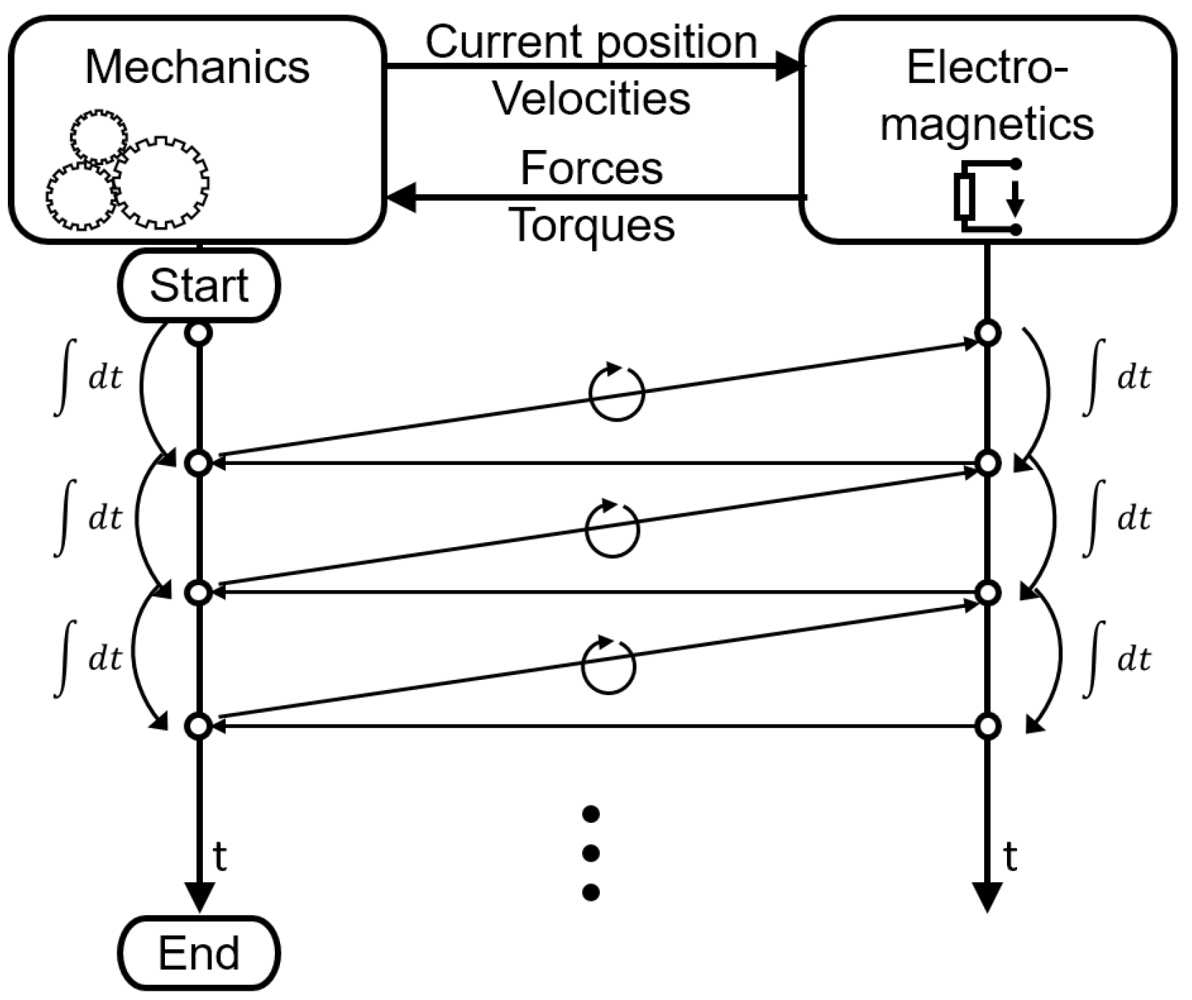
Figure 1 shows a possible implementation of a strong two-way coupling. The mechanical system performs a time integration step $dt$ and calculates the displacements and velocities at the end of the time step. These are handed over to the electromagnetic system, where a time integration step of the same length with the solution of the previous time step as initial condition is performed. The resulting electromagnetic forces combined with the displacements, velocities, and accelerations are checked for convergence of the time step for the whole system. If needed, the time step calculation is repeated until the tolerance criteria is fulfilled.

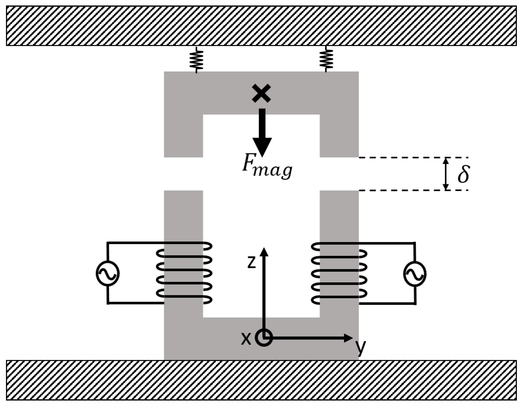
To test the presented implementation, a simple example is needed. A simple example of electromagnetism is given with two iron cores in U-profile with a small air gap and coils around one of the iron cores for induction. This example is well known in literature. Combined with springs counteracting the electromagnetic force, an electro-mechanic system is created. The setup is illustrated in Figure 2.

This test case enables the verification of the implementation of the coupling, as the general behavior can still be estimated from basic physical understanding. Furthermore, building this test case as a test bench to measure the system behavior is feasible. Section 4 explains the measurement setup, and Section 5 shows the comparison results of measurements and simulations, using this test case.

The scope of this work is to validate the aforementioned coupling. To keep the analysis simple, only vertical movements of the hanging iron core are investigated. As shown in Figure 2, this is defined to be the z-direction. The x- and y-axes are defined accordingly, with the x-axis pointing out of plane. The study of the z-DoF is sufficient, as the methodology can be extended to further DoFs without adaptions. Cross-couplings between the directions are covered automatically with the presented method when extending the DoFs.

The coupling is intended to be independent of the geometry of the structural or electromagnetic parts. Therefore, the displacements, velocities, forces, and torques are handed over as integrated, scalar values at the center of gravity of the moving body. The cross in Figure 2 indicates this point for the given test case. This assumption can be used as a multi-body-solver that solves for a rigid body, and distributed forces are only relevant to flexible bodies.

In case a body can not be assumed as rigid, the coupling itself is not affected. Deformations in flexible bodies can be seen as energy dissipation. Additionally, they can influence the behavior of the electromagnetic field. Therefore, a coupled analysis of electromagnetic field and structural mechanics needs to be performed before handing over the resulting integrated force to the multi-body solver. This increase in complexity will naturally increase the computation time and should be used when the accuracy of the resulting force is significantly impacted by the deformation.

To capture static and dynamic system behavior, direct and alternating current are used for system excitation. With the direct current, the steady state of the system in simulation and measurements can be tested. The alternating current leads to a sinusoidal excitation force acting on the system. With this analysis, the dynamics of the coupling can be validated.

3. Numerical Setup to Model Interactions

In the following, the used software and the implementation of the coupling are explained in more detail. This is followed by the description of the model preparation for a coupled simulation.

3.1. Software

In wind energy, several tools are commonly used to model wind turbines. These tools have to include aerodynamics and structural dynamics. For offshore applications, hydrodynamics also have to be included. For generator modeling, most of the models use a simple look-up table representation of generator speed and generator moment depending on wind speed and pitch angle to represent the electrical behavior. The generator is mainly modeled as part of the drive-train, simplified to a two-mass torsional spring-damper-system.

One common code for this kind of wind turbine simulation is the open source code OpenFAST [7]. To extend its modeling depth and include further parts into the system, massive coding effort is needed. Another widely used software for wind turbines is Simpack, as shown in [23]. This software offers high flexibility in the system definition, and additional parts or degrees of freedom can be added easily using the Simpack user interface. With future investigation, the DoFs relevant to electro-mechanical interactions have to be identified. Therefore, the flexibility of Simpack is important. The study is based on Simpack v2021. Additionally, Simpack offers the user to extend the functionality by writing so-called UserRoutines.

These UserRoutines allow defining, e.g., new force elements. The implementation is possible in Fortran or C; here, C was used. The recommended use is to include external data to the simulations, which fits the need for the wanted coupling. The possibility to manipulate the time integration process by adding an intermediate convergence check is especially helpful for this study.

To model the electromagnetic behaviour of the system, Comsol Multiphysics 5.6 [22] is used. The software is a general multiphysics software with solvers for many applications, including electromagnetism. Comsol offers features for external model control via Matlab or Java. Using the Java interface, a Java class, loading and manipulating a Comsol model and running simulations, can be created. This offers the possibility to flexibly load the Comsol model of interest and implement a model-independent coupling.

To interface the C code of the Simpack UserRoutine and the Java class controlling the Comsol model, the Java Native Interface (JNI) is used. Using JNI, the Simpack UserRoutine loads the compiled Java class and hands over the name of the Comsol model to load for the coupled simulation. A reference to the loaded Java class is stored in the UserRoutine and is addressed at any time when communication between the tools is needed.

3.2. Coupling Schema

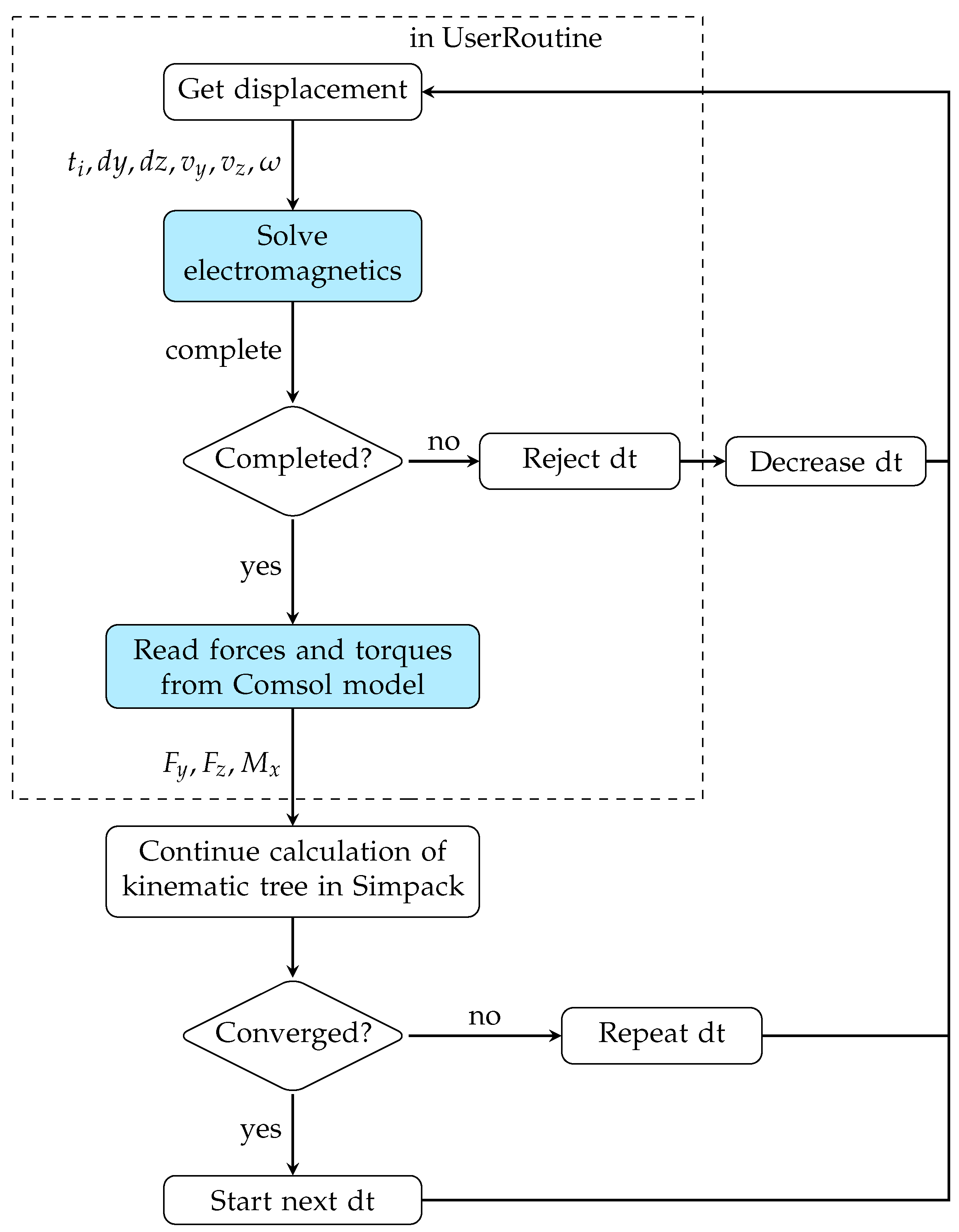
As already mentioned in Section 2, displacements, velocities, and the time step information have to be handed over from mechanical to electromagnetic side. Forces and torques resulting from the magnetic field are returned. To ensure the overall convergence, checks at different points in the simulation workflow are needed. The solutions of both models have to converge for each time step separately, and additionally the whole system has to converge.

Figure 3 shows the flow chart of the implemented workflow. Simpack is controlling the time integration, deciding about time step $dt$ and the system convergence. Therefore, on the Simpack side, no further implementations are needed. The general convergence check of Simpack is used to control the mechanical part and the whole system simultaneously. Comsol also controls the convergence of its time integration automatically. If the Comsol time integration stops for convergence reasons, an error feedback is sent to Simpack. If the Comsol solution did not converge, a time step rejection is thrown by the UserRoutine to notify Simpack that the time step did not converge and a repetition of the time step with smaller step size is needed. If a smaller step size in Simpack is impossible, the coupled simulation breaks.

On the Simpack side, the joint of the anchor only allows vertical movements in z-direction. To enable the movement of the anchor in Comsol, a moving mesh setup is used, using the displacement given by Simpack as input.

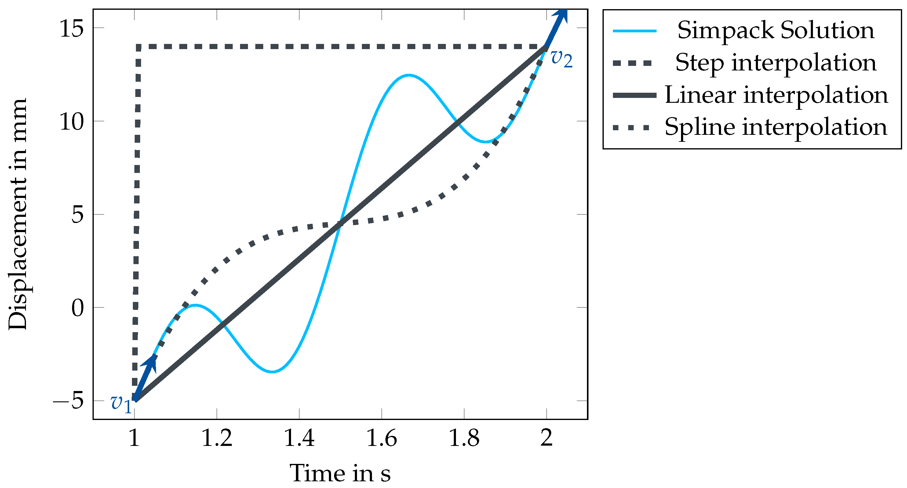
As Simpack is providing the displacement at the end of the time step and the states of the former time step are used as initial condition, an interpolation for the integration of this time step in Comsol is needed. Possible interpolation methods are, e.g., step function, linear, polynomial, and spline interpolation.

Figure 4 illustrates the resulting movement functions for a fictitious Simpack solution (blue). Using the step function (dashed line), the time integration in Comsol was unstable during dynamic interactions. This might be caused by the discontinuity at the step. Using linear (solid line) or spline (dotted line) interpolation, the coupled simulations are stable. The linear interpolation only needs the values at the start and end of the interval. The spline interpolation additionally needs the derivatives at both points (blue arrows $v_1$ and $v_2$) to solve for the four coefficients of a cubic polynomial and achieve a C1-continuous function. For this coupling, the relevant quantity of interest is the velocity of the moving body, which can be provided by Simpack. A polynomial interpolation would need additional values from the former time steps, depending on the degree of the polynomial, which increases the needed storage. Therefore, this option is not investigated here.

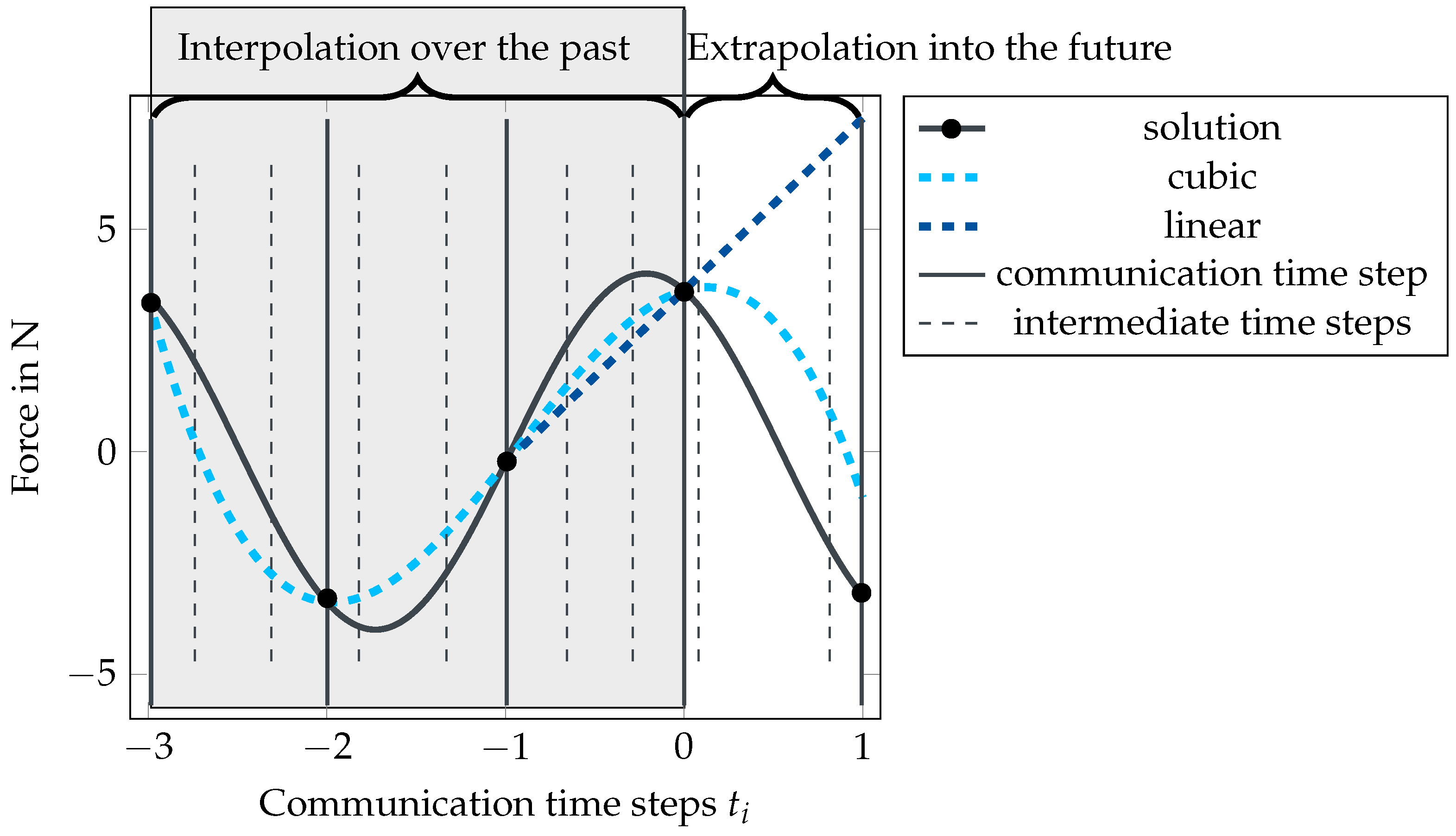
The finite element simulation of Comsol is computationally expensive, and in case of many short time intervals, many time-consuming initialization runs are needed. This can cause a simulation with 1 s simulation time to take between 10 min and 8 h depending on the time step. Simpack, on the other hand, is using variable time steps that may become very small for nonlinear problems. To limit the number of Comsol calls, a fixed communication interval is introduced. Simpack still needs electromagnetic forces at the intermediate time steps. This is illustrated in Figure 5 with the light gray dashed vertical lines. To fill these intermediate steps, an extrapolation of the Comsol solution up to the next communication time step is needed.

Extrapolation methods are widely used in fluid structure interaction simulations [24], and an investigation of their applicability to electro-mechanical interactions is needed. The simplest option is constant extrapolation, meaning that the solution of the last time step is kept, similar to the step function for interpolation. A second option is the linear extrapolation using the two last time steps as interpolation points (see Figure 5 dark blue dashed line). Higher order options increase the number of needed former time steps. Similar to the interpolation, polynomials can be used for extrapolation. Here, quadratic and cubic extrapolation were investigated. The cubic extrapolation is also shown in Figure 5 (light blue dashed line).

Higher order extrapolation methods need several former time steps as interpolation points. Therefore, they can only be applied after several communication intervals. To overcome this restriction, a ramp up of the extrapolation method to higher order during the first time steps was implemented.

The possible improvement of performance, keeping the simulation stable, is dependent on the combination of chosen convergence tolerance, the size of the communication interval, and the interpolation and extrapolation method. A detailed performance and accuracy study for the introduced options is presented in the next subsection.

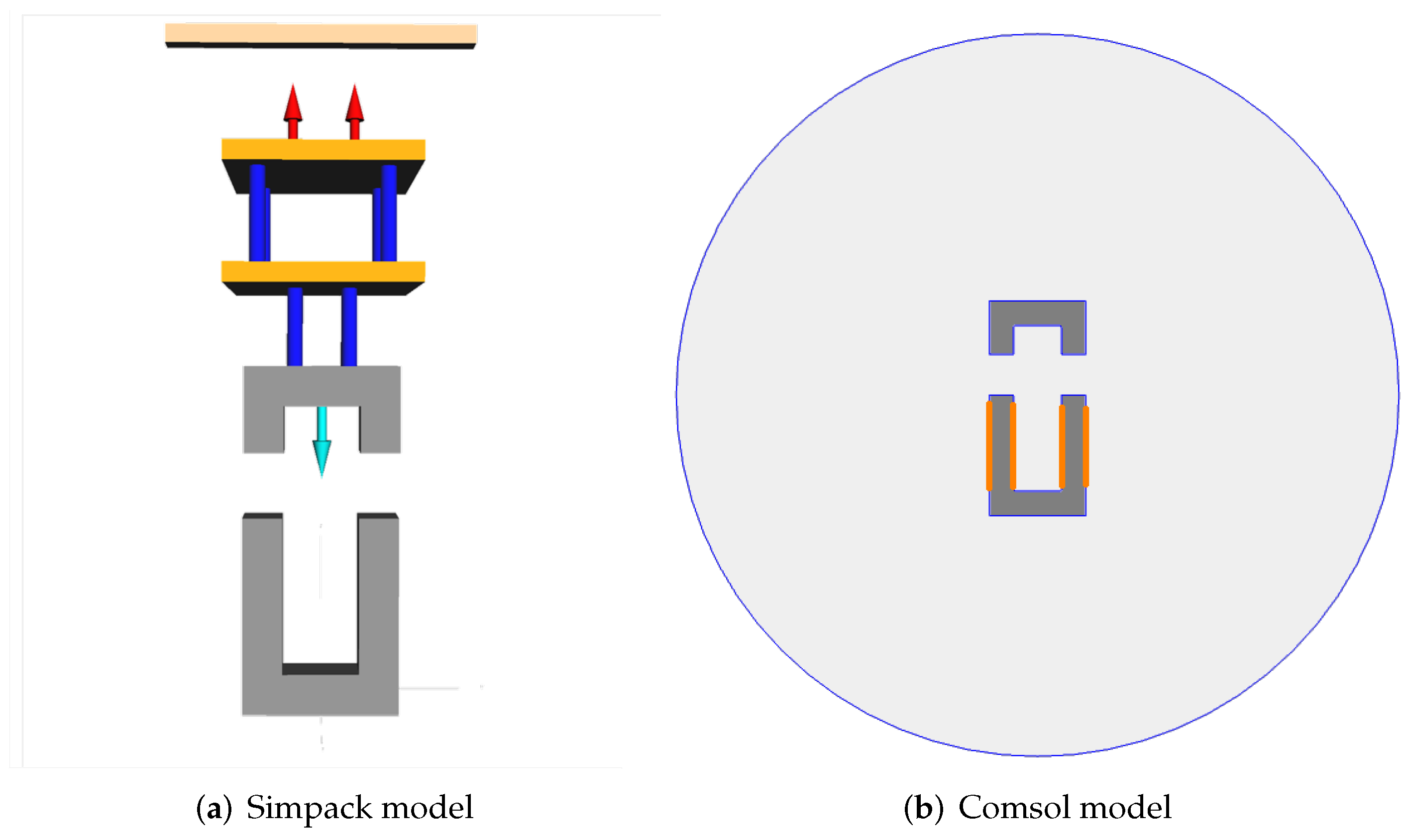
3.3. Model Preparation

The test setup, explained in Section 2, was implemented as simulation models in Simpack and Comsol, as given in Figure 6. The additional parts above the upper iron core are needed to keep the metal springs out of the magnetic field in the measurement setup. Details are explained in Section 4. The red arrows in (a) indicate the position of the springs and their reaction forces. The light blue arrow marks the position of the electromagnetic force. The springs are modeled as force elements with a linear spring stiffness. The electromagnetic force results out of the presented coupling. All bodies are modeled in Simpack as three-dimensional bodies with mass and mass moment of inertia. In Comsol, a two-dimensional model is chosen to reduce the computational effort. The coils are modeled as boundary conditions on the lower iron core, indicated with orange lines. The upper iron core is modeled with a moving mesh to allow the movements of the body during time integration. As physical environment, the magnetic field formulation is used.

For Simpack, the solver was set to “SODASRT 2”. This solver is based on the implicit backward differentiation formula (BDF) [25] and, according to the Simpack documentation, it is a very robust and fast solver. For Comsol, the implemented BDF solver [26] did not converge in all cases; especially for highly deformed mesh, the solver failed. Better robustness was reached with the available “generalized alpha” solver [27]. Here, a free time stepping was chosen. The solver was using a fully coupled formulation with a constant Newton method for damping. The constant damping factor over all iterations was set to 1. The chosen settings are expected to be problem-dependent and need to be adapted especially for more complex systems.

Initially, a mesh convergence study and a mesh optimization for the Comsol model is performed. The most relevant value to be handed over from Comsol to Simpack is the magnetic attraction force in z-direction. Therefore, this value is used as convergence tolerance. As mesh quality measures the skewness of the elements, according to the Comsol, documentation is used [28]. The resulting triangle mesh with 2314 elements has an average element quality of 0.799.

Both Simpack and Comsol, are using adaptive time steps, so the user specifications about time steps only influence the output time step of the results, but not the time integration. That is why a time step convergence study is not needed for this coupling.

The adaptive time step in both programs is influenced by the chosen tolerance criteria. Comsol is set to “scaled tolerance”, using the tolerance criteria given in Equation (2). The equation is dependent on the number of fields M, counted with j and the DoFs $N_j$ for each field, counted with i. The solver estimates the local absolute error of the scaled solution vector $Y_i$, given with $E_{Y_i}$. $A_{\mathrm{s},i}$ represents the scaled absolute tolerance criteria and R the relative tolerance criteria. The time step is accepted if the condition of Equation (2) is fulfilled, otherwise the time step is decreased.

Simpack checks for convergence according to Equation (3). $\Delta s_i\left(t\right)$ is the effective tolerance of the current value $s_i\left(t\right)$ for the $i^{th}$ element in the state vector. The chosen tolerances are included with $\Delta s_{\mathrm{abs},i}$ as absolute tolerance and $\Delta s_{\mathrm{rel},i}$ as relative tolerance. The time step is decreased until the changes of the values $s_i\left(t\right)$ are within $\Delta s_i\left(t\right)$.

Therefore, a convergence study on tolerance criteria is needed additionally to the mesh convergence study. This study needs to be combined with the study on the suitable communication interval. At first, the communication interval was kept small with $\Delta t=$ 0.001 s and only the tolerance was studied. The tolerance was set to ${10}^{-1}$ for relative and absolute values in Simpack. Comsol was kept with default values. Stepwise, the absolute and the relative tolerance were divided by 10, until the simulation results for time integration showed no visible changes. The procedure was repeated several times, increasing the communication interval in steps up to 0.04 s. Additionally, the methods of interpolation and extrapolation were varied according to a full factorial study.

$$\sqrt{\frac{1}{M}\sum _j\frac{1}{N_j}\sum _i{\left(\frac{|E_{Y_i}|}{A_{\mathrm{s},i}+R\left|Y_i\right|}\right)}^2}<1$$

(2)

$$\Delta s_i\left(t\right)=\Delta s_{\mathrm{abs},i}+\left|s_i\left(t\right)\right|\Delta s_{\mathrm{rel},i}$$

(3)

Accuracy and performance were analyzed. The resulting parameters for the testing example are listed in

Table 1. List of optimal coupling configuration for investigated example.

Investigated Criteria	Chosen Method or Value
Simpack tolerance	${10}^{-4}$ in general and ${10}^{-7}$ for positions
Comsol tolerance	${10}^{-4}$
Communication interval	0.04 s
Interpolation method	spline
Extrapolation method	cubic

. The resulting performance with a four-thread solver achieves 8 min per second of simulation. The accuracy is shown in the validation section.

The described implementation is independent of the geometry of the investigated problem. Therefore, it enables the study of electro-mechanical interactions with various configurations and for any combination of generator type and wind turbine. Studies for optimal coupling setup are, however, problem-dependent and need to be repeated with every new physical problem.

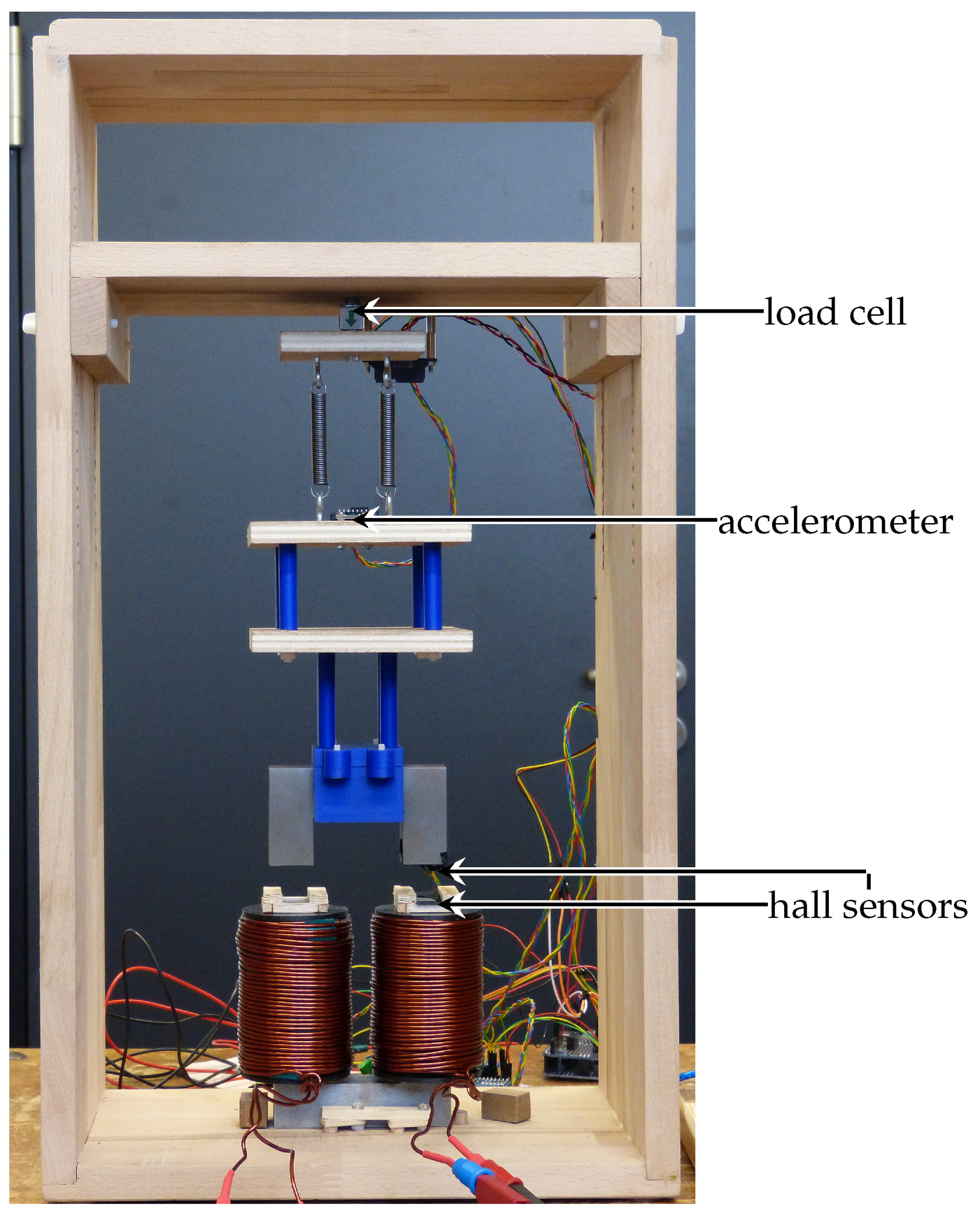
4. Experimental Setup to Measure Interactions

For the validation of the presented coupling, the test case as described in Section 2 was built with measurement equipment. The setup is shown in Figure 7. The anchor and stator are 10 cm wide and 2.5 cm in depth. The anchor is 5.5 cm high, and the stator is 12.5 cm high. The overall height of the frame is 55 cm and the frame is 35 cm wide.

Compared to the basic setup in Section 2, some adjustments were necessary. To avoid any influence of the springs on the magnetic field between anchor and stator, the anchor was hung on a suspension made of wood and 3D-printed plastics. This suspension includes two horizontal wooden plates, which add damping due to the airflow around them when moving. This results in the need for an extra force element in the mechanical model, following Equation (4) for the resulting drag force acting on the system. The big horizontal wooden plate above the marked load cell is adjustable in height. This allows to change the steady-state air gap length and increases the flexibility for validation cases.

$$F_{\mathrm{D}}=\frac{1}{2}\rho A{c}_{\mathrm{D}}{v}^2$$

(4)

To measure the dynamics of the test bench, sensors were applied to the system. The imprinted current is measured with a sensor connected between the current source and one of the coils. The sensor uses a Hall sensor parallel to the wire to measure the current amplitude. The resulting magnetic flux densities on stator and anchor side are measured with two Hall sensors, as indicated in Figure 7. The force acting on the anchor is measured with the load cell at the top. This way, the load cell measures the gravitational force and the total force of both springs. Additionally, the dynamic behavior can be measured with a three-axis accelerometer mounted on the anchor suspension (see Figure 7).

All devices are connected to an Arduino Uno for logging. The output signals of load cell, Hall sensors, and current sensor are sent through an analogue digital converter before reaching the Arduino. The Arduino is running with an average sampling rate of 10 ms. To ensure an equidistant signal, the measurement time series is linearly interpolated. All sensors include measurement tolerances, leading to uncertainty in the measured values. This is important to keep in mind when comparing the values to simulation results.

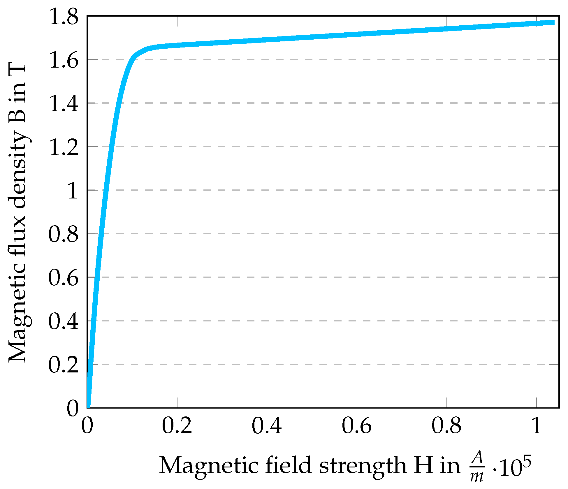
In addition to the sensor tolerances, the measured system properties such as mass, stiffness, damping, and material properties of magnetic flux density B and magnetic field strength H in the B–H curve introduce uncertainty as well. The hanging iron core and its suspension were put on a scale. The springs were characterized using a tensile test bench. The magnetic properties of the magnetic circuit were determined according to IEC 60404-4 [29].

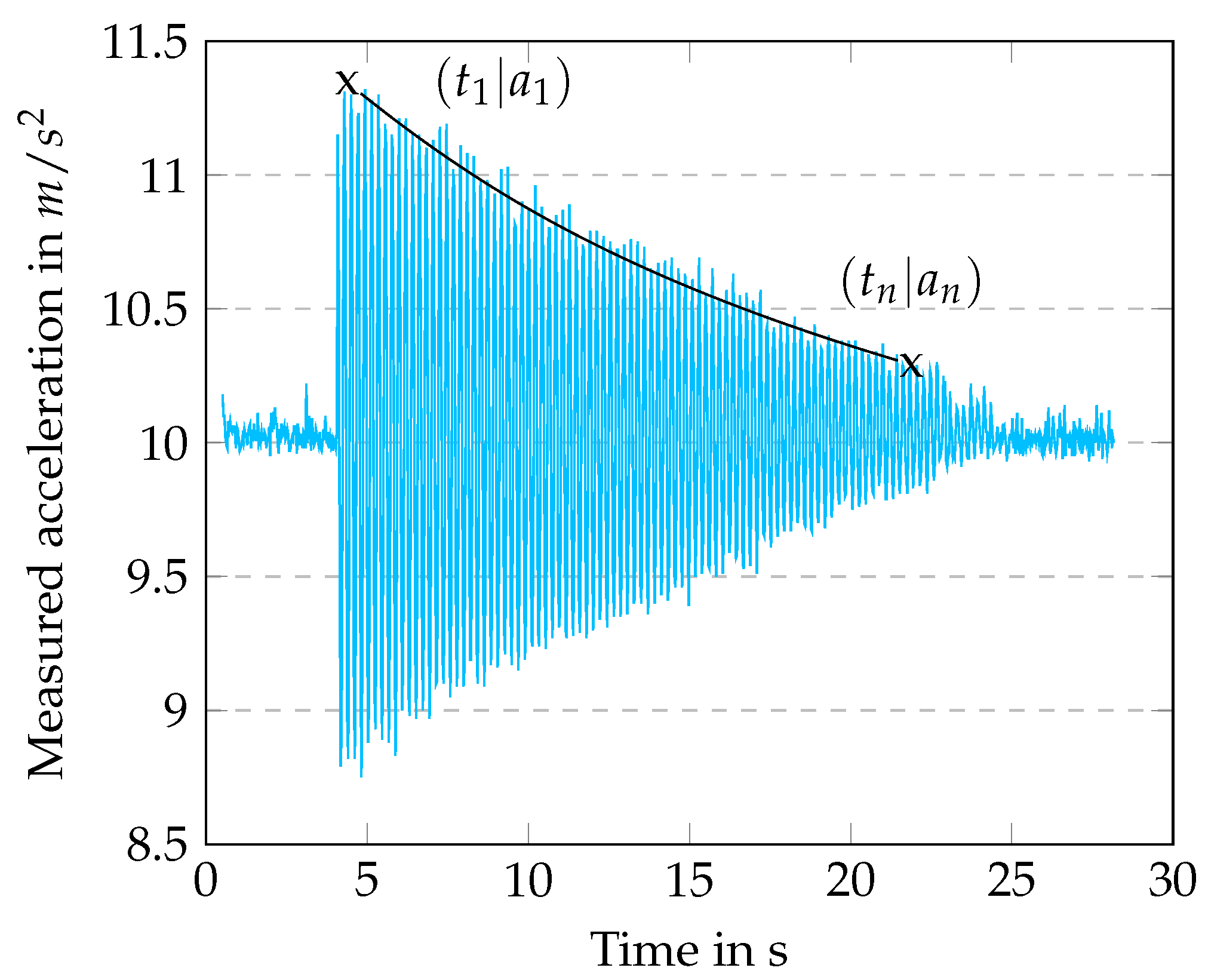
Using a step excitation and recording the system’s response, as shown in Figure 8, the system damping d was calculated according to Equation (5) from the logarithmic decrement $\Lambda$ from the amplitudes $a_1$ and $a_n$, where n symbolizes the number of cycles between the two. From the equation, it also can be seen that the system damping is dependent on the moving mass m and the system stiffness $k=2\ast k_{\mathrm{S}}$.

To account for the measurement uncertainties, all measurements of system properties were performed three times. The resulting mean values were used as inputs for the simulation models. The determined values are given in Section 5.

$$\begin{array}{cc}\hfill d& =2\sqrt{mk}\frac{\Lambda }{\sqrt{{\left(2\pi \right)}^2+{\Lambda }^2}}\hfill \\ \hfill \mathrm{with}\Lambda & =\frac{1}{n}ln\left(\frac{a_1}{a_n}\right)\hfill \end{array}$$

(5)

5. Validation of the Electro-Mechanical Interface

In this section, the used validation cases and the results of the comparison of simulation and measurement are presented.

5.1. System Parameters and Validation Cases

The exact input parameters for the simulation are given in

Table A1. Set simulation model system properties according to measured system properties of test bench.

System Property	Value	Unit
Mass m	1.100	kg
Spring stiffness of one spring $k_{spring}$	480	$\frac{\mathrm{N}}{\mathrm{m}}$
System damping d	0.06	$\frac{\mathrm{Ns}}{\mathrm{m}}$
Number of coil turns N	432	-
conductor diameter	2	mm
Drag coefficient of quadratic plate $c_{\mathrm{D}}$	1.11	-
Aerodynamic effective area A	0.0144	m${}^2$
Air density $\rho$	1.225	$\frac{\mathrm{kg}}{{\mathrm{m}}^3}$

in Appendix A. Figure A1 in Appendix A additionally shows the B–H curve which was input to Comsol. All values have been measured as described in Section 4. The comparison results for the validation in the Section 5.2 are based on these values.

Table 2. Measured validation cases with direct and alternating current, varying current magnitude I, and initial air gap length ${\delta }_0$.

Case No.	I [A]	f [Hz]	${\mathit{\delta }}_0$ [mm]
1	2	-	23.0
2	2	-	42.5
3	4	-	23.0
4	4	-	42.5
5	2	2	23.0
6	2	2	42.5
7	3	2	23.0
8	4	2	42.5

lists the load cases investigated in this study. The cases 1 to 4 were used to analyze the steady states of the system, using direct current (DC) for excitation. The current magnitude was set to 2 A and 4 A with initial air gaps of ${\delta }_0=$ 23 mm and 42.5 mm, respectively.

The cases 5 to 8 use alternating current (AC) for system excitation to analyze the dynamic system behavior. The used current magnitudes were the same as for the DC cases, and the used current frequency was set to 2 Hz. This results in a 4 Hz excitation of the magnetic field, as the magnetic flux density alternates with twice the frequency of the current. The excitation is close to the natural frequency of the system, which can be calculated from the mass and system stiffness according to Equation (6). The difference between the two frequencies avoids direct resonance, which could be harmful to the test bench.

$$f_0=\frac{\sqrt{\frac{2k_{\mathrm{S}}}{m}}}{2\pi }=4.7\mathrm{Hz}$$

(6)

5.2. Validation Results and Discussion

5.2.1. Static Analysis

The validation of the implemented two-way coupling is done in two steps. The first step focuses on the static behavior of the system. Having brought the test model to steady state, the direct current ramps up to the wanted magnitude and the system behavior is recorded until the new steady state is reached. For each case, three independent measurements are performed. The dark gray bars in Figure 9 show their means and uncertainty. Equations (7)–(9) describe the calculation process to derive minimum, maximum, and mean value, as shown in the plot. The blue bars in Figure 9 show the simulation results.

$$F_{\mathrm{mean}}=mean(F_1,F_2,F_3)$$

(7)

$$F_{\min }=min(F_1-{\Delta }_{\mathrm{tol}},F_2-{\Delta }_{\mathrm{tol}},F_3-{\Delta }_{\mathrm{tol}})$$

(8)

$$F_{\max }=max(F_1+{\Delta }_{\mathrm{tol}},F_2+{\Delta }_{\mathrm{tol}},F_3+{\Delta }_{\mathrm{tol}})$$

(9)

${\Delta }_{\mathrm{rel}}$ denotes the relative difference of simulation and measurement normalized to the measurement result. In each case, the relative difference is less than 4% and, except for case 3, the simulation is inside the error margin of the measurement. The differences in case 3 may result from the other system uncertainties. A list of uncertainties included in the test setup and their explanation is given in Appendix A. All in all, the comparison proves that the static behavior of the system is well captured by the coupled simulation.

5.2.2. Dynamic Analysis

To study the dynamic behavior, the system was brought again to rest in the mechanical steady state. Then, an alternating current with a frequency of 2 Hz, starting at 0 A, was introduced to the system, according to Table 2 cases 5 to 8. Again, the measurements for each case are run three times.

The comparison of measurements and simulation is carried out at first using time series results. The averaged time series from the experiment is compared to the simulation result. Figure 10 shows an example time series for the two cases, 5 (subplots (a) and (b)) and 8 (subplots (c) and (d)). Analogous to Equations (8) and (9), the minimum and maximum boundary of the acceleration measurement are determined. The gray area around the mean denotes the tolerance band. For readability, a magnified detail of the plot is given on the right in subplot (b) and (d). It shows that for case 5, the amplitude is slightly higher than the mean measurement, and in case 8, the amplitude is slightly lower. Nevertheless, the simulation always stays within the measurement tolerance for both cases.

To better understand similarities and differences of the measurements and simulations, a fast Fourier transformation (FFT) is applied to the signals. The comparison of the power spectral densities for both cases are given in Figure 11 and shows a clear agreement of the dominating frequencies at 4 Hz and 4.7 Hz. The peak at 4 Hz is caused by the current excitation, as the magnetic field oscillates with twice the frequency of the current of 2 Hz. The 4.7 Hz represents the natural frequency of the system according to Equation (6). Additionally, the simulation results show peaks at 8 Hz and 12 Hz. They can be interpreted as higher order harmonics of the excitation frequency. They can also be observed in the experiments, but at lower intensity owing to damping effects not captured by the simulation.

The last measure to compare measurement and simulation results is the cross correlation. It determines the correlation factor between the two signals for different time shifts between the signals. Figure 12 shows the cross correlation for the simulation and experiment for cases 5 and 8. From subplots (a) and (c), it is visible that the highest correlation is achieved around zero in both cases. Figure 12b,d give a magnified detail plot onto the region. For case 5, the highest correlation factor is achieved for a time shift of 0.04 s. This means that the simulation result is running 0.04 s after the measurements. The shift could be a result of the uncertainty in signal synchronization. For case 8, zero time shift gives the highest correlation factor. Both correlation factors’ maxima are above 0.8. Usually, 0.7 is considered to be a boundary value for strong correlation [30]. Therefore, the signals show strong correlation.

Taking into account the uncertainties of the model inputs and the measurement devices, together with the high correlation factors, the coupling is considered as validated for simulations of general electro-mechanical interactions.

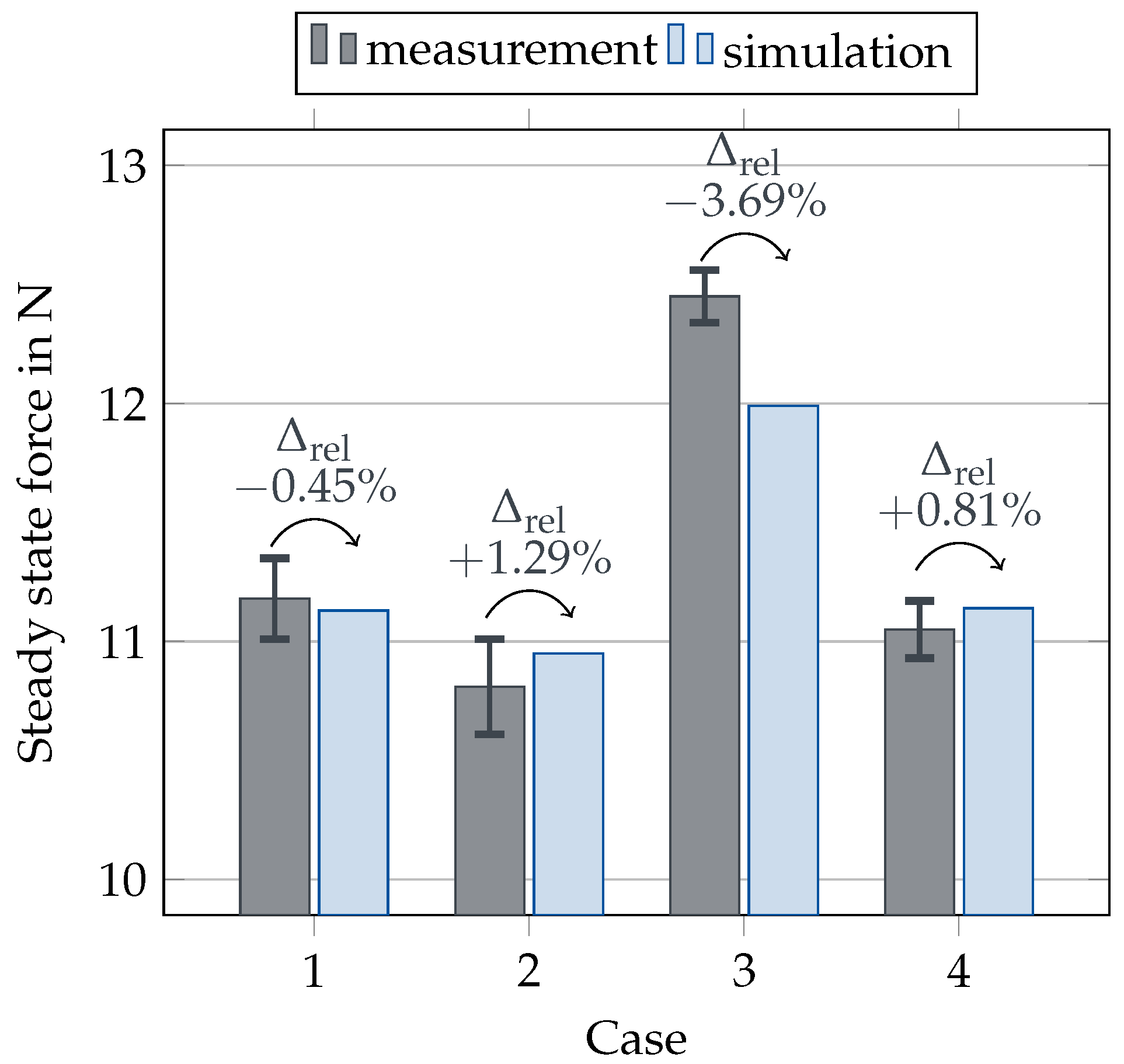
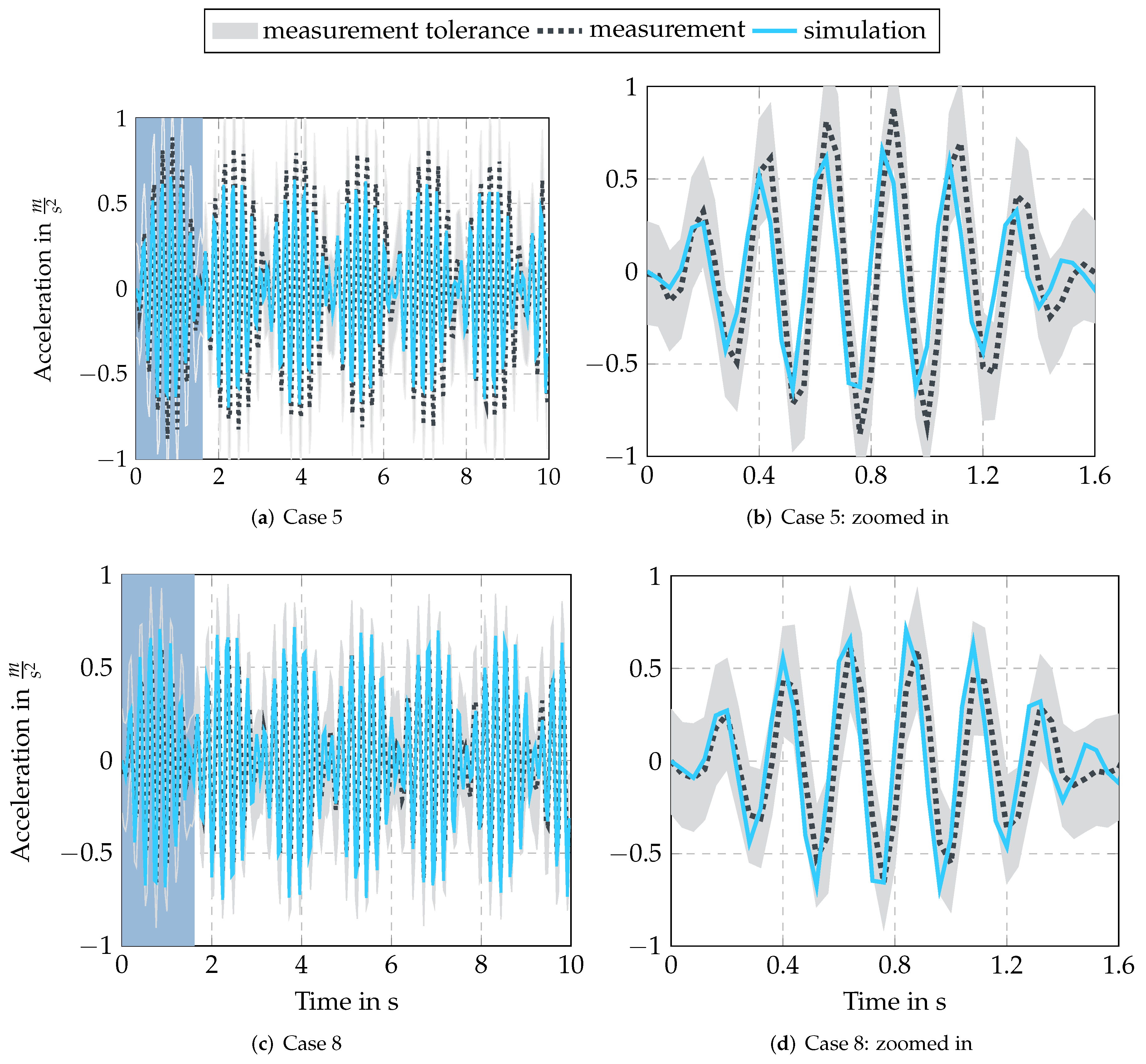
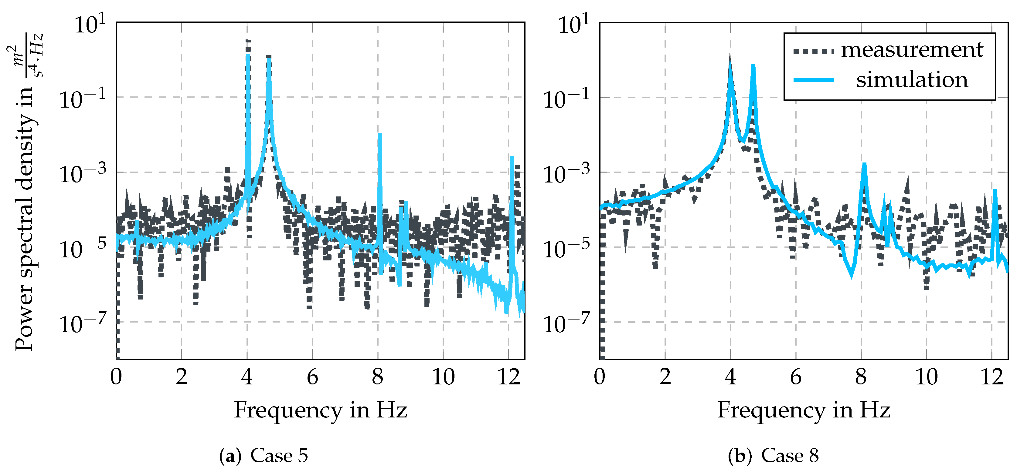
6. Conclusions

The numerical implementation and testing of a new two-way coupling for electro-mechanical interactions is introduced in this paper. The coupling allows the communication of a multi-body simulation solver with a finite element solver for electromagnetic physics. The present solver time and the displacements and velocities of the investigated body are handed over from the multi-body solver to the electromagnetic solver. The electromagnetic solver returns the resulting electromagnetic forces and torques to the multi-body solver. As the multi-body solver neglects deformations, the interface reduces to scalar values. This simplification allows using the introduced coupling for any electro-mechanical problem with rigid bodies, independent of the actual use case. The extension to flexible bodies in electromagnetic fields can be achieved by adding a solver for structural mechanics to the component model. The interface to the multi-body solver, presented here, is not affected.

Furthermore, numerical aspects of the coupling implementation are discussed. Investigated parameters to speed up the coupled simulation are the tolerance criteria of both solvers and the communication strategy. A fixed communication interval between the two solvers in combination with interpolation and extrapolation methods for intermediate steps can lead to a significant speed-up.

The optimal behavior was achieved with spline interpolation and cubic extrapolation. Nevertheless, this is expected to be problem-dependent. The used tolerance criteria are of minor importance for the performance of this implementation.

To validate the implementation of the two-way coupling, a test setup with two U-shaped iron cores was built and measured. The parameters of the test setup were determined and input into the model. Static and dynamic behavior of the system of measurements and simulation are compared and show good agreement. Based on the results presented, the two-way coupling introduced with this study can be considered as validated.

The benefits of the presented coupling are as follows:

• The possibility to analyze, in principle, any electro-mechanical system.
• The possibility to analyze interactions between the mechanical and the electrical side of the system in both directions (two-way coupling).
• Dynamic system analyses, e.g., stochastic system excitation.
• The possibility to include transient system behavior for multi-body and electromagnetic components, e.g., eddy currents.

Therefore, the presented work contributes to future enhanced analysis of electro-mechanical interactions, especially—but not limited to—wind energy.