1. Introduction
Data center energy efficiency has become of crucial importance in recent years due to its high economic, environmental, and performance impact. For example, the leading petaflop supercomputers consume a range of 1–18 MW of electrical power, with 1.5 MW on average, which can be easily translated into millions of dollars per year in electricity bills [
1]. Data center energy consumption was estimated to be between 1.1% and 1.5% of worldwide electricity usage in 2010 [
2,
3], generating as much pollution as a nation such as Argentina [
4]. In some cases, the power costs exceed the cost of purchasing hardware [
5]. Furthermore, the energy costs of powering a typical data center doubles every five years [
6]. Therefore, with such a steep increase in power use, electricity bills have become a significant expense for today’s data centers [
7,
8]. For these reasons, data center energy efficiency is now considered a primary concern for data center operators, often ahead of the traditional considerations of availability and security.
There are several approaches for green computing, from electrical materials to circuit design, systems integration, and software. These techniques may differ, but they share the same goal—to substantially reduce overall system energy consumption without a corresponding negative impact on delivered performance. The processor and main memory are the components that usually dominate power consumption, as shown in
Figure 1. The processor can consume as much as 50% of the total energy [
9,
10,
11]. For that reason, modern processors incorporate several features for power management [
12,
13,
14,
15], such as dynamic power management (DPM) and dynamic voltage and frequency scaling (DVFS). DPM encompasses a set of techniques for obtaining energy-efficient computing by deactivating or reducing the system components’ performance when they are idle or partially utilized [
16,
17]. DVFS allows the frequency and voltage to be adjusted in run-time depending on current needs.
DVFS is motivated by the well-known fact that frequency and power have a near-cubic relationship [
1,
2]; this implies that running the CPU at a lower frequency causes a linear reduction in performance and a near-cubic reduction in power, which could lead to a near-square reduction in CPU energy. Because of this, it is possible to achieve dramatic energy savings just with frequency control, depending on the system and its architecture. Although very promising, the system software has yet to determine when and what voltage and frequency to use when running applications. Otherwise, not only will performance deteriorate, but, in the worst case, energy consumption would also increase [
1]. Indeed, reducing the frequency results in a longer execution time, which increases the energy consumption of other system components, such as memory and disks. There is also an overhead of time and energy associated with a voltage and frequency switch that needs to be considered. Thus, finding the most appropriate voltage and frequency to use in all circumstances is not easy. Therefore, since its introduction in 1994 [
1], there has been a tremendous amount of research on DVFS algorithms.
The DPM technique can achieve substantial energy savings on systems where the static power is high, or the system remains inactive for a long time. In that case, the problem is to determine when and which components to turn on/off. With DPM, energy savings of 70% have been reported [
16,
17].
However, at the same time, while these power-saving techniques reduce system energy, they can compromise performance leading to a complex trade-off that needs to be carefully exploited to produce more energy-efficient algorithms. Indeed, this study investigates whether the construction of an energy consumption model of an application can lead to significant energy savings.
We propose an analytical energy model for a given application in the function of the two control variables present in most HPC systems: CPU operating frequency and number of active cores. The model is composed of three application-dependent parameters and three parameters relating to the architecture of the system. The application parameters incorporate characteristics of the percentage of parallelism and the input size. The system architecture parameters include power-related and technology-dependent components, such as dynamic, static, and leakage power.
The main contributions of the proposed model are:
Simple model: faster to fit and compute, good for DVFS and DPM optimization.
Parameters with logical meaning: helps to understand the contribution of each specific term.
Analytical analysis: several analyses can be derived from the equation.
Controllable variables: the equation is in the function of parameters that we can control directly.
We have organized the rest of this paper in the following way. In
Section 2 and
Section 3, we present a general review of existing models showing the differences between each approach and their applications. In
Section 4, we propose our model and derive its parameters alongside its constraints. In
Section 5, we validate the model with the PARSEC benchmark applications. Further on, in
Section 5.8, we present use cases of the model, as well as how we applied it in DVFS algorithms. Finally, we conclude with a discussion in
Section 6.
2. Related Work
Merkel et al. [
18] developed an energy model for processors based on events. Their model assumes a fixed energy consumption
for each activity, and by counting the number of occurrences
of every activity, they estimate the total energy as:
Another event-based model, introduced by Roy et al. [
19], described the computational energy consumed by a CPU for an algorithm
A as the Equation (
2)
where
is a processor clock leakage power,
is the total execution time,
is the total time taken by non-I/O operations, and
is used to capture the power consumption per operation performed by the CPU.
and
are estimated using performance features.
Models based on events present some drawbacks, they are highly dependent on the operating system and its architecture, making them problematic to port for other platforms. There are also limitations regarding the number of simultaneous events that can coexist without adding a non-negligible overhead. Additionally, there are cases where events need multiplexing, for example, when using more hardware events than the CPU can provide. There are also some well know problems regarding the precision of some events, as shown in many studies [
20,
21,
22,
23,
24,
25]. Some events that should be exact and deterministic (such as the number of executed instructions) show run-to-run variations and over-count on various architectures, even when running in strictly controlled environments. Because of that, our proposed model is not dependent on events and, therefore, not vulnerable to those drawbacks.
An instruction-level energy model was also proposed in [
26] by Yakun et. al. Where they proposed an energy per instruction (EPI) characterization made on Xeon Phi. Their model is expressed as:
where
N is the total number of dynamic instructions,
is the initial idle power,
is the average dynamic power, and (
−
) refers to the cumulative number of cycles the micro-benchmark performs. This model is suitable for estimating the energy after the application finishes executing when it is possible to count the total cycles. However, it is challenging to use for optimization or forecasting since it does not have an application model to predict the cycles. Our model integrates the behavior of the application, taking into account the execution time.
Lewis et al. [
27] described the overall system energy consumption using the following equation:
where,
,
,
, and
are unknown constants that are calculated via linear regression analysis and those remain constant for a specific server architecture. This model, as the previous one, relies on knowledge of energy spent on each component, being a suitable option for estimation after the application has already run, but not for optimization of the run itself, which is the aim of our model.
In another energy consumption model based on system utilization, Mills et al. [
28] modeled the energy consumed by a compute node with CPU (single) executing at speed
as Equation (
5)
where
stands for the overhead power consumed regardless of the processor speed,
and
are the application’s initial and final execution times. The overhead includes power consumption by all other system components, such as memory, network, and more. For this reason, although the authors mentioned the energy consumption of a socket, their power model is generalized to the entire server. This model lacks a closed-form, i.e., it depends on the definition of
to be complete. Our model has a closed-form which facilitates analyses.
Although much work has been done on DVFS, the focus is still on the consumer electronics and laptop markets. For HPC, the notion of energy perception is relatively new [
29]. Moreover, the operational characteristics of non-HPC and HPC systems are significantly different. First, the workload on non-HPC systems is very interactive with the end-user, but the workload on the HPC platform is not. Second, activities conducted on a non-HPC platform tend to share more machine resources. In contrast, in HPC, each job often runs with dedicated resources. Third, an HPC system is usually much larger than a non-HPC system, making it more challenging to gather information, organize, and execute global decisions. Therefore, it is worthwhile to investigate whether a DVFS scheduling algorithm, which works well for conventional computing, remains effective for HPC.
Our paper proposes a full-system energy model based on the CPU frequency and the number of cores. The model aims to understand and optimize the energy behavior of parallel applications in HPC systems according to application parameters, such as the degree of parallelism and CPU parameters related to dynamic and static power. The proposed model differs from existing ones, including the frequency and number of cores in the same equation for estimating the energy for a specific application in a given configuration. This model can serve as a base for considering DVFS and DPM optimization problems, including frequency and active cores. It can also be used to analyze the contribution of each parameter (ex: level of parallelism) to energy consumption. Furthermore, the number of cores is essential in HPC since applications are designed to run on multiple cores.
The proposed energy model is the product of an application-agnostic power model and an architecture-specific application performance model. The power model is based on the CMOS logic gates power draw as a function of the frequency [
30,
31] augmented to include the number of cores. The performance model is based on Amdahl’s law [
32,
33,
34], which can be used to estimate runtime in multi-core systems. In addition, this model has been extended to include execution frequency and input size, characterizing the application on the target architecture.
Table 1 summarizes the models comparing the system dependencies and the controllable variables.
3. Theoretical Background
A model is a formal representation of a natural system. The representation of computer system models includes equations, graphical models, rules, decision trees, representative collections of examples, and neural networks. The choice of representation affects the model’s accuracy, as well as its interpretability by people [
35,
36,
37]. Accurate energy and power consumption models are essential for many energy efficiency schemes employed in computing equipment [
5], and they can have multiple uses, including the design, forecasting, and optimization of data center systems. This study focuses on analytical models that could aid energy optimization and analyses of crucial factors in the total energy draw.
The desirable properties of a full-system model of energy consumption include accuracy, speed, generality and portability, inexpensiveness, and simplicity [
38]. However, modeling an HPC system’s exact energy consumption behavior is not straightforward, either at the whole-system level or at the level of individual components. Data centers’ energy consumption patterns depend on multiple factors, such as hardware specifications, workload, cooling requirements, or the type of the applications. Some of these factors cannot be measured easily. Furthermore, it is impractical to perform detailed measurements of the energy consumption of lower-level components without additional overhead.
Several proposed models have already been classified concerning their input parameters, as shown by Dayarathna et al. [
2], who analyzed more than 200 models according to their characteristics and limitations and classified them into categories where the model is more suited to its objectives:
System utilization or workload
Frequency
Other system states, such as cache miss, branch prediction, number of instructions executed, and more
Often, energy models are described as a combination of two main parts, the power model of the system and the performance model of the application. This is because the concept of energy (E) is the total amount of work performed by a system over a period of time (T), while power (P) is the rate at which the system performs the work. The relation between these three amounts can be expressed as:
3.1. Power Models
The modeling of system parameters is becoming popular nowadays with the advantage of performance counters provided by the CPU or the operating system. These counters can measure micro-architectural events, such as instructions executed, cache hits, miss-predicted branches, and more; thus, providing a base for many different estimations of power usage. This makes this type of model very suitable for power estimation because it can use information about several internal states of the computer.
Frequency-based models are the most common kind of model. They serve as a base for many power models [
30,
31,
39]. These models utilize the fact that every digital circuit (including modern processors) is composed of transistors. Thus, modeling one transistor’s interaction and scaling this to the chip can give a reasonable estimate of the entire system’s energy. One of the most common frequency-based model approximations is defined as follows:
where
and
are model parameters, and
f is the operating frequency (details of this equation are covered in
Section 4). This type of model is suitable for optimization problems since these are a function of the operating frequency, which can be easily controlled.
3.2. Performance Models
The most common way to model the application performance is using the workload. The workload is an abstract representation of the amount of work done for a given time and speed. The workload (
W) can be defined in many different ways. One common way, used in many studies, such as Paolillo et al. [
40], Francis et al. [
1], and Kim et al. [
41], is the following:
where
is total active time, and
s is the execution speed in instructions/second.
Utilization models [
1,
42] are also found in the literature, defined as the ratio between the time that the system is active and the total time (idle and active). These models are present in many DVFS algorithms present in Linux. They can be viewed as a good alternative to the workload since it is impossible to measure workload in real-time. Equation (
9) defines workload in terms of CPU utilization (
u):
where
T is the total execution time (idle and active), and
is the active time, meaning when the processor was executing instructions. Models based on CPU utilization are the basis for DVFS algorithms. Even though this is not a controllable parameter, it is straightforward to measure system utilization with almost no overhead, and it is also very portable in terms of operating systems and architectures.
5. Experimental Validation
In this section, the models presented in
Section 4.1 and
Section 4.2 were validated with a benchmark specific for multi-core architectures. Additionally, in order to assess the modeling overhead and accuracy, our proposal was then compared to machine learning approaches. We compared against support vector regression (SVR) [
50], decision tree [
51], k-nearest neighbors [
52], multilayer perceptron [
53], and some new methods, such as Gao et al. [
54]. However, SVR was chosen as the most representative because it performed best in our tests without aggressive fine-tuning, as shown in
Figure 2.
5.1. Case Study Architecture
The experiments were executed in one computer node equipped with two Intel Xeon E5-2698 v3 processors with sixteen cores each and two hardware threads for each core. The maximum non-turbo frequency was 2.3 GHz, and the total physical memory of the node was 128 GB (8 × 16 GB). Turbo frequency and hardware multi-threading were disabled during all experiments. The operating system used was Linux CentOS 6.5, kernel 4.16.
The Linux kernel has many different policies for power management, depending on the driver. In the default driver, the acpi-cpufreq, the options are Powersave, Performance, Ondemand, Conservative, and Userspace. Each governor has a policy on how the frequency is selected. In this investigation, the frequency control was performed using the Userspace governor, which allows the user or any userspace program to set the CPU to a specific frequency. The core control was accomplished by modifying the appropriate system files with the default CPU-hotplug driver.
The architecture was equipped with the intelligent platform management interface (IPMI), a set of interfaces allowing out-of-band management of computer systems and platform-status monitoring via the local network [
55]. It can monitor variables and resources, such as the system’s temperature, voltage, fans, and power supplies, with independent sensors attached to the hardware.
5.2. Case Study Applications
The applications blackscholes, bodytrack, canneal, dedup, fluidanimate, freqmine, raytrace, swaptions, vips and x264 from the PARSEC
https://parsec.cs.princeton.edu/download.htm (accessed on 20 February 2020). parallel benchmark suite, version 3.0 [
56], OpenMC [
57] and LINPACK (HPL) [
58], were chosen as case studies. The PARSEC benchmark focused on emerging workloads and was designed to represent the next-generation shared-memory programs for chip-multiprocessors. It covers an ample range of areas, such as financial analysis, computer vision, engineering, enterprise storage, animation, similarity search, data mining, machine learning, and media processing. The OpenMC and the LINPACK are two classic HPC programs.
5.3. Verifying Hypothesis
In this section, we validate whether the assumptions of our model are valid for the system used.
5.3.1. Frequency and Voltage Relation
One of the assumptions was that the frequency and the voltage have a linear relationship, as indicated by Equation (
12). To verify that, we build an experiment that sets the frequency to a specific value while sampling the voltage using the APERF and MPERF registers that provide feedback on the current CPU frequency. The average result of the sampling voltages is shown in
Figure 3, where we can observe a near-perfect linear relation. This is because manufacturers implement this curve in the processors, using tables that relate ranges of frequencies to voltages so that they can precisely define any curve that will better suit their design.
5.3.2. Input Size and Instructions
We ran the applications with different inputs assuming linear growth in the amount of work for one input to the other when building our model. However, measuring and controlling the amount of work would require much instrumentation and tuning to find an input corresponding to a certain amount of work. Therefore, to build our models, we use the time to reference the amount of work, assuming that the work is proportional to the executing time.
Figure 4 corresponds to the verification of this supposition.
Table 2 shows that the assumption was reasonable since the average correlation was 0.96 for all applications, indicating that growth in the number of instructions will follow the time. This was the case for all applications that we ran in our benchmark and should hold for any data parallelism type of application.
The next assumption was that the application’s behavior was the same when varying the workload. This condition is necessary for using the model with an unknown input size because, if the behavior is the same, we can interpolate the known inputs. One way to verify this is to measure the rate of instructions per second normalized by the frequency, as shown in
Figure 5.
Figure 5 shows that the applications have roughly the same curve when normalized; this also happens for all other applications in our benchmark.
The final assumption is that the workload should also not vary depending on the number of cores or frequency. To verify, we measure the total number of executed instructions while varying the cores from 1 to 32.
Table 3 shows the results.
Table 3 shows the standard deviation and what that corresponds to in terms of the total number of instructions as a percentage.
The same test was performed for the frequency, varying from 1.2 to 2.2 GHz with 100 MHz steps. The results are shown in
Table 4.
These results show that all the assumptions were reasonable, and we can safely move to the validation of the model’s prediction.
5.4. Fitting the Models
To find the parameters of Equation (
22), 10 uniformly random configurations of frequencies (
f), cores (
p) and inputs (
N) were chosen from the range
,
and
, respectively. The application was executed for each chosen configuration, and the measured energy and time values were collected. For the input size, if we assume that all CPU instructions take approximately the same time to execute, the number of basic operations will be directly correlated with the time. Thus, we can estimate the input size by looking at the execution time, allowing us to divide a large input size into several smaller ones, knowing their relationship, as performed in the work of Oliveira [
49]. The unity can also vary depending on the definition. For simplicity, we assign numbers from 1 to 10, increasing the problem linearly, so it is also possible to interpolate any input in between these values.
For each configuration, samples of the power were collected using IPMI every 1 second. This sampling rate was chosen based on the magnitude of the mean run time of the applications, which is in the order of minutes. Therefore, this rate provides enough samples to measure average power. Additionally, timestamps and the total run time were collected. The total energy spent on each configuration is estimated by first interpolating the power samples using the first-order method and then integrating this function in the time.
The model’s parameters are calculated by solving an optimization problem of finding the values that minimize the squared error of the prediction to the measured values using the non-linear least-squares method.
The Python library Scikit-Learn was used to build the SVR model [
59]. The SVR was trained using the same data used for parameter estimation of equation (
22) with a grid search used to find the best kernel function and the best values for the hyper-parameters penalty for the wrong (
C) and (
). For this data, the best function was the radial base function (RBF), and the hyper-parameters were
and
.
5.5. Measured versus Modeled Energy
To validate the model, we ran all possible configurations in the tested machine, varying the cores in a range of
, the frequency in
, and the input in
. The total number of configurations varies from 400 to over 1000 depending on the application, as some applications have restrictions on the number of cores that they can run. Once the data was collected, we computed the mean percentage error (MPE) according to the following equation:
5.5.1. Frequency × Cores
Figure 6 plots the measured and modeled energy consumption for some of the applications modeled. In addition, some of the possible shapes that the model can take while varying the number of active cores, and operating frequency, are shown.
5.5.2. Frequency × Input
Figure 7 plots the measured and modeled energy consumption for some of the applications modeled. The diagrams show some of the possible shapes that the model can take while varying the operating frequency, and input size.
5.5.3. Cores × Input
Figure 8 plots the measured and modeled energy consumption for some of the applications modeled. The diagrams show some of the possible shapes that the model can take while varying the number of active cores, and input size.
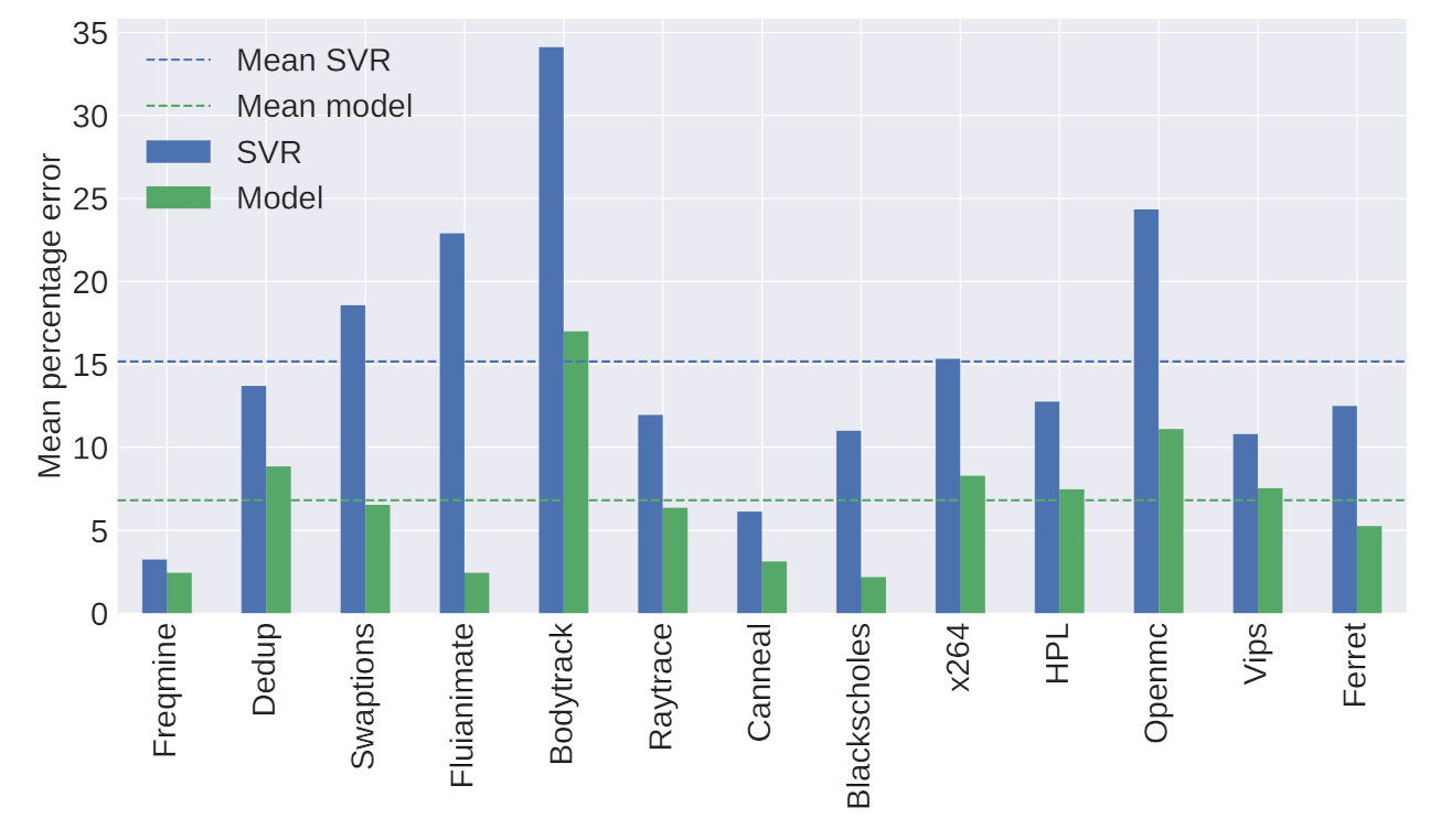
5.5.4. Validation
The average results for each application were calculated using a model trained with only 10 configurations, and the comparison is displayed
Figure 9.
Figure 9 shows that the proposed model always performed better, with a lower MPE than SVR, when we were limited to 10 training points. This result is further explored in the next
Section 5.6, where we undertake a comparison with different training sizes.
5.6. Overheads on Training
It is known that machine learning is data-driven; in that sense, the SVR model obtained using only 10 configurations could be improved, but what about the analytical model? To answer that question, the proposed model and the SVR were also trained with a varying number of configurations. We then compared the MPE and the amount of energy spent to create each model. This accuracy-energy trade-off is crucial since building models’ energy overhead defeats the primary goal of saving power when running applications.
Figure 10 shows the comparisons of MPE and energy spent to create each model for two selected applications. According to the results, the analytical model is very stable, not changing much as more data is added, while the SVR keeps reshaping to adapt to the data. The error of the analytical model is almost constant but that of the SVR, initially very high, drops as more data is used in the training process.
Figure 11 presents the overall results, with the mean energy overhead and MPE for all applications. The meeting point of the MPE for the SVR and the proposed model can be extracted from
Figure 11b. It shows that, in around 90 configurations, the SVR starts to have a smaller error. The cost of that is the linear increase in energy spent on training. The increase in energy, about 10 times more, can be observed in
Figure 11a.
5.7. Analysis
One of the most significant advantages of using an analytical model is the understanding of the problem that an equation provides, making many different kinds of analysis possible that are otherwise impossible with a machine learning model. In this section, we discuss one of the possible analyses. In the following figures, we try to understand the contribution of each parameter of the equation to the total energy consumption.
For this analysis, we took the model of one of the applications and, varying one parameter of the equation, we display the energy versus performance (time) for all configurations. After that, we computed the Pareto frontier, a set of all Pareto efficient allocations, i.e., all the configurations where resources cannot be reallocated to make one individual better off without making at least one individual worse off. This gives us all the configurations where we have an optimal trade-off of performance and energy to choose from.
Figure 12 shows the Pareto frontier for several values for the static power parameter (
in Equation (
22)) with configurations of frequency ranging from 1.2 to 5 GHz and cores from 1 to 64, so that we can also have an idea of what is the tendency when we increase the frequency and number of cores.
From this figure, we can see that when increasing the value of the static power parameter, the total energy consumption increases as expected. We can also observe that the values that minimize the total energy consumption tend to be high frequency and multiple cores. This is one of the consequences of increasing the static power factor. As the dynamic factor proportionally decreases, its variables tend to have less impact on total consumption, enabling configurations with high frequency and several cores. This also enables chip-level optimization for choosing components that change the ratio between static and dynamic power.
Figure 13 shows the Pareto frontier in the same ranges described before but for the parameter corresponding to the level of parallelism of the application (
w in Equation (
22)).
In
Figure 13, we observe that, as the parallelism level increases the total energy decreases. The number of cores tends to be higher with a higher level of parallelism as expected, and the frequency shows an inverse relation.
5.8. DVFS and DPM Optimization
The effectiveness of the proposed approach during optimization was evaluated with a simple algorithm that finds the optimal frequency and number of active cores from the proposed equation. The results were then compared to the Linux default choices for power management.
With Equation (
22), it is possible to calculate energy consumption estimates for each possible configuration since there is a finite range of possible values for the frequency and number of cores. It is also possible to apply constraints on the execution time, frequency, and the number of active cores. Then, the configuration that minimizes energy consumption for a given input can be selected. The complete workflow is shown in
Figure 14. We can see that any optimization problem can be structured with our model and the system’s constraints. In the following examples, the optimization problem that we build is to minimize the energy equation given the constraints of possible frequencies and the number of cores that our system can run. The algorithm selected to minimize was the newton-CG [
60].
Current HPC managers leave to the user the choice of how many cores to use. On this basis, three situations were analyzed in relation to the number of cores:
Worst choice: number of cores that maximize the total energy consumed;
Random choice: energy consumed for a random choice of the number of cores;
Best choice: number of cores that minimize the total energy consumed (oracle).
The default option for the Linux governor is Ondemand, and, by default, it has no DPM control for the number of active cores. As Ondemand only performs DVFS, for comparison, each application was executed with all available cores in the system, from 1 to 32.
Figure 15,
Figure 16 and
Figure 17, show the energy savings with respect to Ondemand, i.e.,
for the three cases described above. The savings and losses for each case are:
Worst choice: save 69.88% on average;
Random choice: save 12.04% on average;
Best choice: lost 14.06% on average.
By default, operating systems do not implement DPM at the core level, and, in HPC, the user usually explicitly chooses the number of cores to run their job. To give a better idea of the impact on the energy consumption of DPM at the core level, we analyzed the choices of the number of cores over a period of one year in the HPC center at UFRN. The result is plotted in
Figure 18.
It is of note that the most common choice of many regular users is a single core requested per job, matching the worst-case choice for all applications analyzed in this investigation. The best choice was quite often 32 cores, which is the third most popular choice among users, but it is 72 times less frequent than 1 core. This led us to envision how much energy could be saved and encouraged us towards future research using the proposed model for DPM or more advanced optimization algorithms.
In practice, this approach can be implemented by allowing the resource manager to perform these changes for the user using pre-scripts and post-scripts for high energy consumption job submissions.
6. Conclusions
This paper proposes an energy model based on the operating frequency and the number of cores for a shared memory system. This model serves as a reference for DVFS and DPM optimization problems.
Results from three different HPC benchmarks demonstrate the potential of the proposed model while consuming 10 times less energy than a machine learning approach, such as SVR, to characterize applications. Moreover, it can provide knowledge-based hints to improve DVFS and DPM algorithms by enabling analysis of the contribution of each model parameter (e.g., level of parallelism) to the energy consumption. Indeed, as shown in
Section 5.8, when no oracle is available to choose the frequency and the number of cores the application should use, the proposed model can save around 12% of energy for a random choice and up to 70% for the worse possible choice. Considering the job history of our own HPC center, which shows the prevalence of worse possible choices made by users, the potential energy savings are very significant and encourage further research.
Although the model is promising, it still has some limitations. The main one is related to the input size, which needs to be estimated to create the application model and optimize the application. Another limitation concerns the power model, which does not consider the load variation, so our model ends up using an average of the energy consumption, which is enough to obtain good results but limits its implementation in real-time optimization. Future research is intended to solve both problems, first adapting the model to use the ratio of executed instructions as input size, something which is more tangible and easy to measure in modern systems without much overhead, and adding new parameters to the power model to account for the load. This would allow us to develop more advanced DVFS models that could identify different phases of a target program with more subtle changes in frequency, and, perhaps, in the number of active cores to further improve the results presented here.


 ,
, 


