Operational Resilience of Nuclear-Renewable Integrated-Energy Microgrids

Abstract

The increasing prevalence and severity of wildfires, severe storms, and cyberattacks is driving the introduction of numerous microgrids to improve resilience locally. While distributed energy resources (DERs), such as small-scale wind and solar photovoltaics with storage, will be major components in future microgrids, today, the majority of microgrids are backed up with fossil-fuel-based generators. Small modular reactors (SMRs) can form synergistic mix with DERs due to their ability to provide baseload and flexible power. The heat produced by SMRs can also fulfill the heating needs of microgrid consumers. This paper discusses an operational scheme based on distributed control of flexible power assets to strengthen the operational resilience of SMR-DER integrated-energy microgrids. A framework is developed to assess the operational resilience of SMR-DER microgrids in terms of system adaptive real-power capacity quantified as a response area metric (RAM). Month-long simulation results are shown with a microgrid developed in a modified Institute of Electrical and Electronics Engineers (IEEE)-30 bus system. The RAM values calculated along the operational simulation reflect the system resilience in real time and can be used to supervise the microgrid operation and reactor’s autonomous control.

1. Introduction

Scientific evidence shows that the frequency and severity of extreme weather events are worsening day by day with global warming, which is harshly impacting the resiliency and integrity of the electrical grid structure [1]. Weather-related power outages account for more than 70% of the total power outages in the U.S. [2]. Between 2003–2012, there had been more than 679 widespread blackouts in the U.S. affecting at least 50,000 customers [3]. More recently, the winter storm Uri in February 2021 resulted in power outages for roughly 10 million people in Texas, causing cascading failure to other facilities relying upon electricity, including drinking water treatment and medical services [4]. It resulted in an estimated $130 billion in damage in Texas alone and reportedly the death of 210 people. Elsewhere outside the U.S., widespread flooding in Queensland, Australia in 2011–2012 resulted in severe damage to transmission facilities causing power disruptions to 150,000 customers [5]. In 2008, a severe ice storm in China resulted in the isolation of 2000 substations and the collapse of 8500 towers leading to power outages in 13 provinces and 170 cities [5].

With centralized electrical grids proving more vulnerable to extreme events, energy consumers are looking to develop microgrids with generation and control capacity to fulfill their demand. Furthermore, microgrids can add value and be compensated for providing power and services to the grid. By aggregating local resources, including energy storage, microgrids can decentralize larger grids into smaller entities, each capable of operating independently when the grid fails. While distributed renewable energy resources (DERs), such as wind and solar photovoltaics (PVs), are central to such microgrid architecture due to their cost-effectiveness and scalability, a large majority of microgrids are backed up with fossil-fuel-based generation (e.g., diesel and natural gas) [6].

There is building interest in replacing fossil generation in existing and instantiating new microgrids with small, advanced nuclear reactors. Small modular reactors (SMRs) are smaller and have increased safety, modularity, and long-lasting fuel, making them more transportable and easier to assemble, lending them to be used in more diverse energy applications [7]. Besides being an excellent baseload generation, SMRs offer flexible power that complements the non-dispatchable generation of DERs to develop diverse and sustainable clean generation mix in microgrids. SMRs are being considered for a wide range of microgrid applications, including military facilities, future space stations and extraterrestrial bases, electric vehicle charging stations, remote communities, virtual power plants, and commercial and industrial facilities [8,9]. SMRs are expected to be available in a variety of sizes less than 100 MWe to fit the needs of the equally diverse size of microgrid applications.

SMRs used as a baseload generation in modern microgrids with high penetration of renewables are shown by Islam and Gabbar in [10] with 24 h hourly dispatch simulation. NuScale’s SMRs are being designed to support flexible operation that includes reactor maneuvering, steam bypass, and dispatching modules individually for multi-module plants [11]. The analysis showed that the SMR alone can absorb a large amount of wind intermittency on a daily basis, albeit sacrificing system economics by controlling steam bypass to meet short-term response. Joshi et al. [12] used dynamic simulations to quantify an SMR’s potential to compensate for intermittency of PV generation in remote microcommunities. The ramp rates and power change limits of SMR were estimated based on operational limits of European nuclear power plants. In [13], the role of electrical energy storage to bridge the gap between flexibility needs and the flexible operation capability of SMRs to support the hosting of PV generation in remote microcommunities is analyzed and quantified in terms of plant load factor. SMRs are designed to provide diverse energy applications, such as seawater desalination [14], oil recovery and refinery [15], hydrogen production, and district heating [16,17], in addition to electricity. Cogeneration, which means supplying both heat and electricity, not only enhances an SMR’s economic potential, adding more impetus towards achieving the carbon reduction goal [18,19], but also boosts its flexible operation capabilities [20,21].

A missing element in the current literature is a tool to consider the required mix and sizing of SMRs, renewable generation, storage, and flexible loads from not only a techno-economic energy basis but also resilience in terms of the magnitude and size of disturbances the system will be designed to withstand. In short, operational resilience must be defined, quantified, and designed into SMR-DER microgrids. To this end, this paper analyzes salient operational features of SMRs to develop a resilience framework and metrics to analyze and quantify the operational resilience of SMR-DER microgrids.

The rest of the paper is organized as follows: Section 2 provides the literature review on operational resilience and discusses the research contributions and novelty of this paper; Section 3 discusses the features of SMR-DER microgrids along with the modeling of microgrid assets, an operational framework for the microgrid control, and the proposed resilience evaluation framework; Section 4 discusses a case study performed in a modified Institute of Electrical and Electronics Engineers (IEEE)-30 bus system (the results discussed include operational quasi-static and dynamic simulations for a 30-day period, resilience sample calculations, and real-time operational resilience quantified in terms of the response area metric (RAM)); Section 5 concludes the paper with proposed future work.

2. Operational Resilience

Currently, the quality of electrical grids is measured by traditional reliability metrics based on system adequacy and security. The reliability-based system planning focuses on low-impact, high-probability events typically characterized by isolated random failures of system components [22]. With extreme weather-related outages becoming more frequent and amplified, it is apparent that this classical approach of system planning needs significant upgrades. Furthermore, the aggressive shift of the power systems towards renewable energy, which themselves are affected by weather conditions, necessitates a new approach capable of reflecting impacts of common-cause failures. Considering its emphasis on extreme disruptive events, the concept of resilience has received significant research attention in the power system domain in recent years.

The concept of resilience was first introduced by C.S. Holling in 1973 as a measure of a system’s ability to absorb disturbances while maintaining unaltered relationships between its components and parameters [23]. Over the years, resilience has been adopted by different domains where it had numerous interpretations and evolutions. Conceptualizing the quantification of disaster resistance against extreme events, multidisciplinary research sponsored by the National Science Foundation utilized the resilience triangle to reflect the loss of functionality after an event and subsequent recovery and restoration [24]. The R4 framework describing robustness, redundancy, resourcefulness, and rapidity of the system against disturbances was introduced to describe system resilience. Cimellaro et al. adopted the resilience triangle to quantify the disaster resilience of hospital buildings [25]. Ouyang et al. extended the resilience triangle into a multi-stage framework by including one additional damage propagation stage between the inception of the event and the start of the recovery [26,27]. The framework was implemented to analyze the extreme event resilience of urban infrastructure systems in [26] and power systems in [27].

In the last two decades, several research works have attempted to define, qualify, quantify, and analyze power system resilience and develop metrics for comparison. References [22,28] define power system resilience as a system’s capability to withstand abnormal high-impact disruptive events including extreme weather events and cyberthreats. References [29,30] further include the operational adaptation as a part of the theoretical definition of the power system resilience. Reference [31] distinguishes the resilience by design and resilience by real-time reaction focusing on disturbances related to cyberthreats. Panteli and Mancarella discussed the influence of extreme events on power system components to provide guidance to develop a modeling framework for power system resilience [32]. They also used the concept of a resilience trapezoid in the context of power systems, breaking the event into preventive, corrective, emergency, restorative, and adaptive stages [5,22]. To quantify the power system resilience with trapezoidal illustration, the “$\Phi \Lambda E\Pi$” resilience metric, pronounced as “FLEP”, was introduced in [22]. Panteli et al. discussed a unified resilience evaluation approach and utilized risk-based defensive islanding to mitigate cascading failures [28].

Chanda et al. discussed a generic code-based metric to quantify the temporal characteristics of power system resilience for an ongoing contingency in a power distribution system [33]. Rieger discussed the quantification of resilience in the context of control systems integrating its physical, cyber, and cognitive aspects [34]. The disturbance and impact resilience evaluation (DIRE) curve was introduced that helped classify a system as resilient or non-resilient based on the attributes reflected in the graph which include robustness, agility, adaptive capacity, adaptive insufficiency, resiliency, and brittleness. Eshghi et al. discussed an agent-based resilience model to develop metrics based on four power system attributes, namely small signal stability, transient stability, communication latency, and sensor physical degradation, recognized in terms of time and data of the measurements [35]. The metrics proposed were intended for the supervisory control and data acquisition system to improve the observability and controllability of the system against for three different classes of disturbances: physical, cyber, and cognitive.

In [29], McJunkin and Rieger used the concept of adaptive capacity to assess and quantify the operational resilience of a modern distribution system (MDS). Instead of focusing on system performance following a disruptive event, the adaptive capacity framework evaluates the system adaptive capacity to respond to such disruptive events. The adaptive capacity refers to the dynamic flexibility of the system expressed in terms of real and/or reactive power to respond to the anticipated disturbances. The adaptive capacity curve has both time and magnitude attributes influenced by the latency, ramp rates, and magnitude of power variation of system assets. Looking forward in time, the magnitude and temporal characteristics of energy-limited and energy-independent assets in a power system are modeled and aggregated to produce system-level adaptive power characteristics that reflect system resilience against anticipated disturbances. In addition to the high-impact disruptive events, the uncertainty in renewable generation (e.g., wind and PVs) and load demands are important issues to consider while analyzing the operational resilience of microgrids hosting large amount of DERs. The adaptive capacity framework analyzes the system reserve to respond to any form of generation–demand imbalance, whether it is from disruptive events or from DER intermittency and uncertainty. This feature of adaptive capacity framework that focuses on system capacity to respond, rather than the consequences of an event, makes it useful to analyze system resilience against uncertainties. In [29], the adaptive capacity curve generated for an MDS is mapped into the DIRE curve to understand the system capability at different stages following disturbances and the roles of different assets in those stages. The operational resilience framework in [29] revolves around the concept of adaptive capacity, which has been implemented for different generation assets. Phillips et al. [36] extended the work in [29] to develop a real-time asymmetric operational metrics by updating the adaptive capacity with control thresholds, contingencies, and environmental conditions and demonstrated the proposed model on a case system for both normal and abnormal scenarios. In [37], Phillips et al. analyzed asset-level flexibility for three classes of hydropower plants, namely, run-off river hydropower, hydropower with reservoir, and pumped-storage hydropower, and developed a framework to integrate their resilience contribution to overall system adaptive capacity characteristics. In [38], the resilience contribution of a hybrid solar PV–battery system was analyzed in terms of adaptive capacity considering the generation uncertainty.

This paper aims to leverage the concept of adaptive capacity in the context of SMRs to develop operational resilience framework for SMR-DER integrated-energy microgrids. The balance between real-power flexibility needs and requirements of SMR-DER microgrids is one of the decisive factors for its operational feasibility. The reactive power, on the other hand, is a generator-centric capability and can also be compensated with localized compensation schemes, such as shunt capacitors and flexible alternating current transmission system (FACTS) devices [39]. Similarly, the power system inertia is based on generator mass and is independent of the energy source driving the prime mover. In other words, the reactive power and inertial model of the SMRs will be similar to other thermal power plants. For this paper, we neglect reactive power and inertia, making the assumption that sufficient inertia or synthetic inertia is present to maintain frequency stability, and sufficient voltage regulation capability is also available. The proposed framework is constructed to assess the operational resilience of an SMR-DER integrated-energy microgrid case system developed for electricity and district heating in a modified IEEE-30 bus network. The major contributions of this paper include:

• A resilience framework based on system adaptive real power of SMR-DER integrated-energy microgrids, taking into consideration the salient operational features of SMRs including flexibility added with cogeneration and the interaction between electrical and the heating system.
• A resilience metric termed as RAM is proposed for anticipated normal and compromised operational scenarios to provide resilience feedback to the microgrid’s asset management system and the reactor’s autonomous control.

The novelty of this research work lies in extending the adaptive capacity framework to model the characteristics of a nuclear system and the complex interaction between heat and power sides for a microgrid’s operational resilience. Compared to earlier resilience works in power systems that mostly focused on modeling power system components, this research explores all three domains of SMR-DER integrated-energy microgrids (i.e., nuclear, heating, and electrical). Furthermore, this research also attempts to characterize the impact of interaction between the heating and electrical sub-systems on a system’s operational resilience. The safety aspect of the nuclear system is added to the resilience model which includes fixed operational pattern and power maneuvering limits of SMR, and real-time decision-making to keep the reactor operating or shut it down based on the disturbance characteristics. The proposed resilience model aims to boost the operational awareness which is critical for SMR-DER microgrids where the flexible assets are limited, and the safety of the nuclear system cannot be compromised. This paper builds on the outcomes of papers that developed a simulation model of an SMR-DER integrated-energy system in [20] and analyzed its optimal design and operation in [21]. The system models and optimization framework from [21] are utilized in this paper to develop and test the operational resilience model of SMR-DER integrated-energy microgrids.

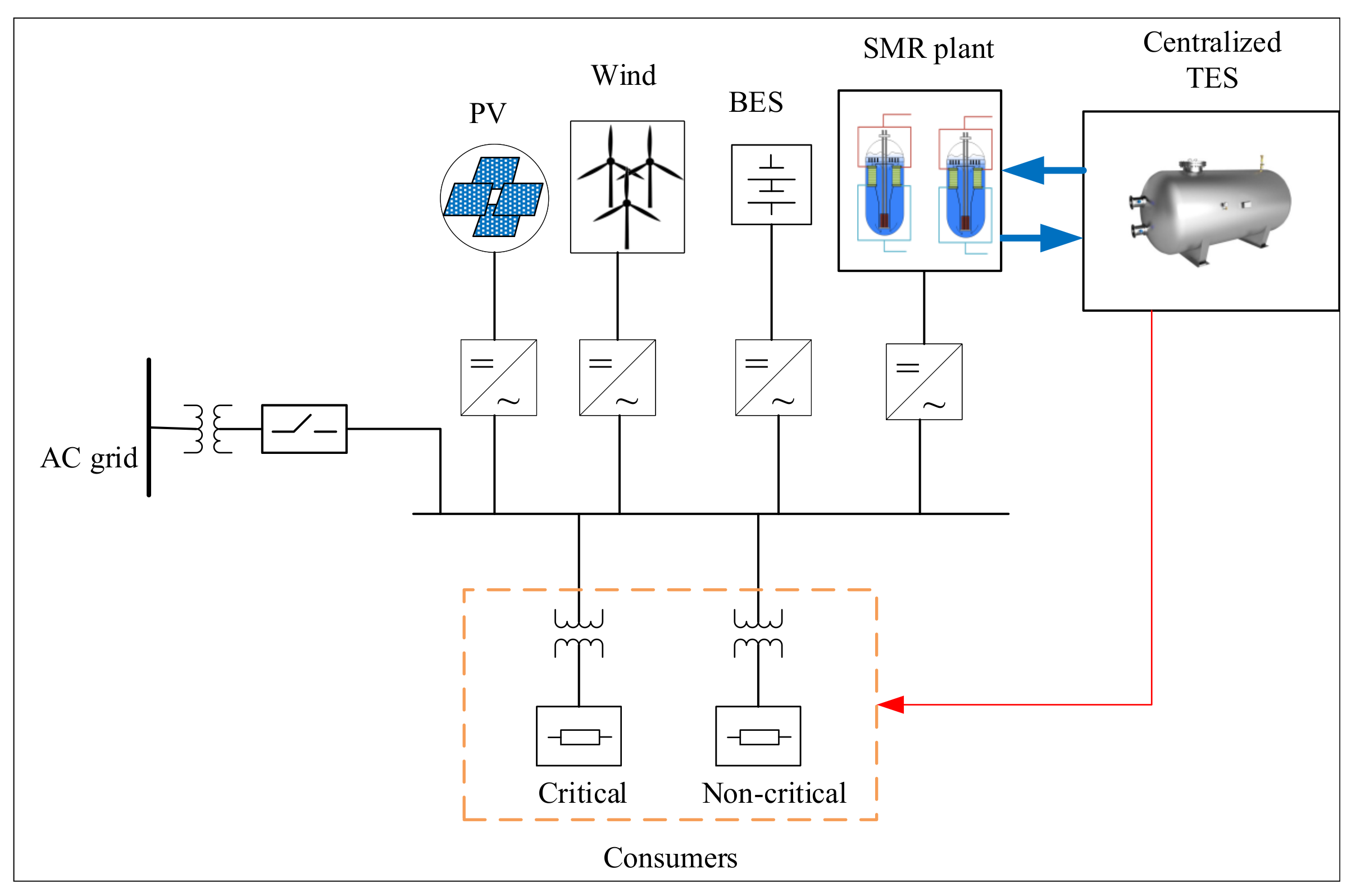
3. System Description

The proposed microgrid system, as depicted in Figure 1, consists of an SMR as the primary source of heat and power and hosts distributed small-scale wind and PV generation. The load in the microgrid can be divided into critical and non-critical loads. One of the assumptions here is that the critical loads cannot be shed, while non-critical loads can be curtailed as required to meet critical load demand. To have the capability to island, the microgrid’s assets are sized to meet, at a minimum, the electricity demand of local critical loads. Additional capabilities can be considered if there is economic value in the potential export of power to the grid. An SMR may be a single-module or multi-module plant based on the availability of sizes to meet the system demand. The sizing of distributed wind and PVs and their pairing with battery energy storage (BES) or other storage mechanisms will be based on an assessment of expected critical load over time profile versus the expected availability and intermittency of the wind and sun. BES can support peak load shaving, support long-term storage, and provide synthetic inertia or primary frequency response. SMR-DER microgrids, as shown in Figure 1, can also meet local heating requirements along with electricity. The steam from an SMR is used to generate electricity and contribute to local heating as needed. The centralized thermal energy storage (TES) will act as a buffer for a heating network to absorb the fluctuations in heating demand and steam supply from a reactor.

Microgrids typically have a limited number of flexible assets to support system operation and respond appropriately to demand fluctuations or local disturbances. Therefore, the sizing of assets and operational strategy chosen will have significant impact on a microgrid’s flexibility. Although SMRs are expected to support flexible operation, they still face technical limitations in terms of their capability to provide flexible power. Frequent operation of control rod for large power changes creates issues such as thermal fatigue and aging of the reactor and thermal components, erosion and corrosion of hydraulic components such as valves and pipes, the core power redistribution, and fission product poisoning [40]. Due to these technical challenges, the reactor control is restricted within the design limits typically defined in terms of the rate of change, the total change, and the total number of large power cycles. Therefore, an SMR’s flexible operation should follow certain operational protocols based on its design limits. In general, an SMR’s salient operational characteristics can be summarized as below [11,40,41]:

• Reactor power maneuvering restricted in terms of total power change, ramp rates, and the total number of power maneuver cycles.
• Non-zero limits on minimum power level in addition to the maximum limits typical to all power plants.
• Fixed standard operating schedule and daily power-cycle to reduce operational uncertainty to maximize system economics and reactor safety.
• Multiple means to provide electrical power change: steam extraction, steam bypass, and reactor control rod maneuvering.

These characteristics are common to SMRs with water/steam in secondary coolant circuit, which represents the majority of current SMR technologies. Note that the design configuration shown in Figure 1 is an example considered for the purposes of this paper. The resilience model developed in this paper for an SMR-DER microgrid with integrated heat application can be adapted to other system configurations, including power-only SMR-DER microgrids. Considering SMRs with the above characteristic features, an operational scheme was introduced in [20] decoupling SMR’s power control into control rod maneuvering, steam extraction, and steam bypass. The simulation results discussed in [21] analyzed the adaptiveness of the operational scheme against uncertainty and intermittency of renewables and showed that an SMR can economically host as much as 50% renewables consisting of wind and PV generation. This paper adopts the operational scheme from [20] to develop the operational framework for microgrid control. The next three subsections discuss the operational framework, modeling of assets, and the resilience framework.

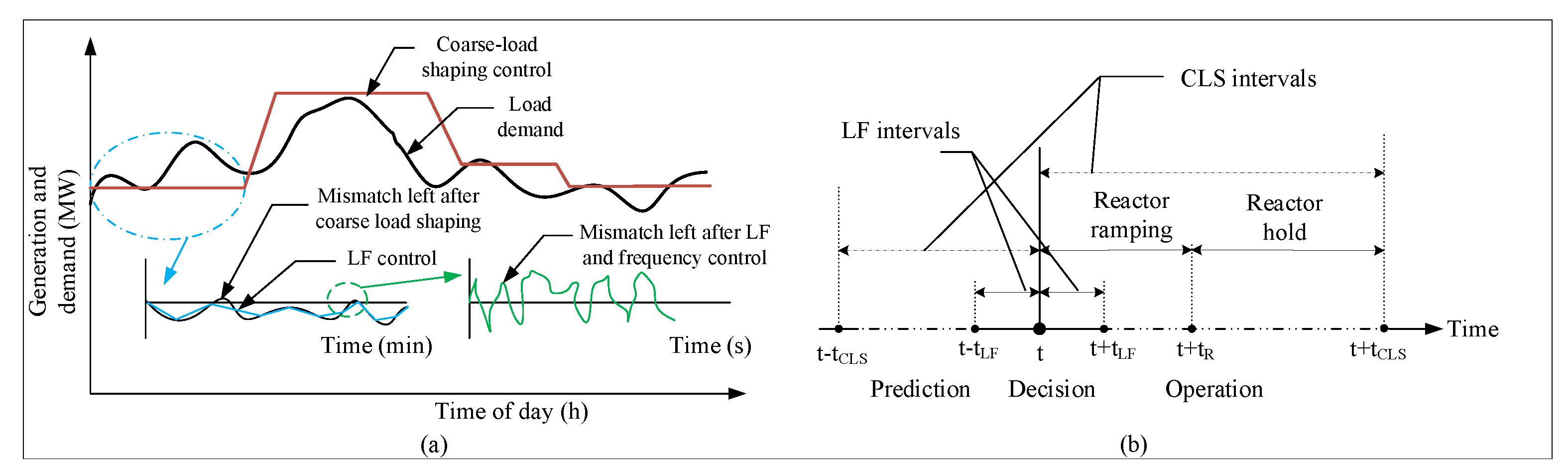
3.1. Operational Framework

The operational framework enables control of all the flexible generation assets to meet instantaneous generation–demand balance. Figure 2a illustrates the distributed control in which overall operation is divided into three parts: coarse-load shaping (CLS), load following (LF), and frequency control (FC). The CLS and LF are setpoint-based controls where operational setpoints are identified beforehand, whereas the FC is automatic control based on instantaneous power system frequency feedback. These three controls are decoupled and are executed in different timescales independently.

Figure 2b shows the real-time operational scheme for setpoint-based controls. The setpoint-based controls (i.e., CLS and LF) are repeated at fixed time intervals. During each interval, the setpoint prediction and operation blocks work in parallel. The prediction block identifies the setpoints for the next interval. The beginning of each interval is referred to as the decision point because it is the moment when the setpoint predicted over the earlier interval has to be executed. The operation block executes the setpoint evaluated by the prediction block at the decision point. The execution of CLS and LF setpoints will bring the generation close to the load demand. FC assets are then operated with frequency deviation feedback to meet the instantaneous generation–demand balance.

3.1.1. Coarse-Loading Shaping

The CLS is the outermost control to coarsely follow the shape of the daily electrical load demand. It is a semi-baseload operation with very few variations per day and with slower ramp rates. It is executed with the help of reactor maneuvering which has strict operational limitations in terms of ramp rate, total change, and the number of reactor maneuvers. In each CLS interval, denoted as $t_{CLS}$, the reactor power level transitions to a new setpoint. The CLS interval or reactor maneuvering cycle consists of ramping and hold periods denoted as $t_R$ and $t_H$, respectively. The reactor ramps to a new setpoint over the ramping period and stays at the new reactor power level throughout the hold duration. For the purposes of this paper, $t_{CLS}$, $t_R$, and $t_H$ are taken as 6 h, 2 h, and 4 h, respectively. The reactor power level setpoints are calculated based on the information analyzed by the decision point. The objective of CLS is to coarsely bring power generation close to demand such that LF and FC can cover short-term fluctuations to ensure instantaneous generation–demand balance. During each CLS interval, the prediction block calculates a new setpoint for the next CLS interval. The CLS prediction block is a mathematical function that captures information, such as predicted electricity and heating demand peaks for the next CLS interval and the loss of state of charge (SOC) of BES and TES, to calculate a new setpoint for the reactor power level. Equation (1) shows the calculation of reactor power setpoint for ${k+1}^{th}$ CLS interval as a function of different state variables and demand predictions:

$$P_{k+1}^{R,th}=f_1(P_k^{R,th},{\widehat{P}}_{k+1}^D,{\widehat{Q}}_{k+1}^D,SO{C}_{k.t_{CLS}}^{TES},SO{C}_{k.t_{CLS}}^{BES}),$$

(1)

where $P_{k+1}^{R,th}$ is the reactor thermal power level setpoint at $k+1^{th}$ interval, $P_k^{R,th}$ is the reactor thermal power level at the $k^{th}$ interval, ${\widehat{P}}_{k+1}^D$ and ${\widehat{Q}}_{k+1}^D$ are the predicted peak electrical and heating demand at the $k+1^{th}$ interval, respectively, and $SO{C}_{k.t_{CLS}}^{TES}$ and $SO{C}_{k.t_{CLS}}^{BES}$ are the SOC of the TES and BES at the decision point, respectively. The SOC of TES is represented by its temperature, and that of BES is represented by the stored energy in pu of the BES energy rating.

If the SMR plant has multiple reactor units, only one unit is maneuvered at a time in each CLS interval. This will help reduce the total number of reactor maneuvers per reactor unit [21]. However, if required, multiple units can operate simultaneously to provide larger power variations.

3.1.2. Load Following

The LF is another setpoint-based control with the interval of $t_{LF}$. For the purposes of this paper, $t_{LF}$ is considered as 15 min. The generation–demand imbalance left after the CLS will be handled with the LF control. In the proposed microgrid configuration shown in Figure 1, the steam produced by the reactor is used for electricity and heat applications. The steam extraction to the heating side can be controlled to achieve power variation on the electrical side. This capability will be used for the LF. In each LF interval, the steam extraction level is changed to a new setpoint value. Meanwhile, the LF prediction block calculates steam extraction level setpoint for the next interval that will meet electrical demand predicted for the next interval. The steam extraction flow setpoint, ${\dot{m}}_j^{EV}$, is therefore a function of the electrical demand predicted over the next LF interval:

$${\dot{m}}_j^{EV}=f_2({\widehat{P}}_j^D),$$

(2)

where ${\widehat{P}}_j^D$ is the electrical demand predicted for the $j^{th}$ LF interval. As mentioned earlier, the LF and CLS are decoupled from each other and controlled independently. Therefore, the sampling indices for CLS and LF (i.e., k and j, respectively) are independent of each other. Note that, unlike CLS interval, LF interval does not have a hold period.

3.1.3. Frequency Control

The setpoint-based controls do not consider the short-term variation within the sampling interval. Furthermore, there could be mismatches left due to the biases and uncertainties in predicted load demand and renewable generation. The short-term generation–demand imbalance left after setpoint-based controls is responded to with instantaneous FC with the help of BES. The BES control will be based on the power system frequency deviation feedback which represents the dynamic generation–demand imbalance. The instantaneous electrical power output of BES, denoted as $P_t^B$, is given as

$$P_t^B=K_{PB}\Delta f_t+K_{IB}{\int }_0^t\Delta f_{t}dt,$$

(3)

where $K_{PB}$ and $K_{IB}$ are the proportional and integral gain of the proportional-integral (PI) controller, respectively. $\Delta f_t$ is instantaneous frequency deviation from the rated frequency.

If BES alone is unable to absorb short-term disturbance, the turbine bypass system, equipped in each reactor unit (see Figure 3), can support the BES by bypassing the process steam directly to the condenser prior to sending to turbine stages (i.e., high-pressure (HP) and low-pressure (LP) turbine stages). Note that the turbine bypass system has different setups than the steam extraction system. The steam extraction system extracts the steam from between turbine stages.

The operation of the turbine bypass system will reduce the reactor’s electrical power and help meet instantaneous generation–demand balance on the power system side. The size and capability of the turbine bypass system may vary with the reactor designs. The NuScale SMR’s turbine bypass system, for example, can bypass up to 100% steam at full reactor power directly to the condenser without shutting down [42]. For the purposes of this paper, the turbine bypass system of the NuScale SMR is assumed. Bypassing a large amount of high-temperature steam for long durations can cause wear and tear of condenser shell and tubes, steam bypass lines, and associated valves. Therefore, the turbine bypass is reserved for certain abnormal scenarios when BES is unable to absorb demand fluctuations. Depending on the disturbance and the anticipated recovery time to return to the normal operation, the reactor unit can remain operating or shutdown on bypass flow at full or reduced reactor power level [42]. The turbine bypass flow is controlled using a simple PI controller, as given by (4).

$$\frac{d{\dot{m}}_t^{BV}}{dt}=\left\{\begin{array}{cc}{K}_{Pbv}\Delta f_t+K_{Ibv}{\int }_0^t\Delta f_{t}dt,\hfill & |\Delta f_t|>\Delta f_{set}\hfill \\ 0,\hfill & |\Delta f_t|<\Delta f_{set}\hfill \end{array}\right.$$

(4)

where ${\dot{m}}_t^{BV}$ is instantaneous bypass flow; $K_{Pbv}$ and $K_{Ibv}$ are the proportional and integral gain of the bypass valve controller, respectively. $\Delta f_{set}$ is frequency deviation threshold or the dead band for bypass valve.

3.2. Asset Models

3.2.1. Small Modular Reactor

The steam produced by the SMR is used for electricity and heating applications. It flows through the bypass valve, HP turbine, extraction valve, and LP turbine before merging at the condenser. The condenser then supplies the feedwater back to the steam generator (SG) through the pump. Figure 3 shows the steam distribution of an SMR with water/steam in secondary coolant cycle.

Note that there could be other components in the secondary coolant circuit in the actual SMR plant, including additional intermediate turbines, moisture separator and reheater between turbines, multiple pumps, and feedwater preheaters and deaerator in the feedwater line [42,43]. The resilience model of an SMR will vary based on the configuration of the reactor system. Specifically, the impact of steam extraction and turbine bypass systems on feedwater preheating and system efficiency needs to be analyzed. However, for the purposes of this paper, the reactor secondary coolant circuit is simplified without reheat and preheat stages assuming an ideal, basic Rankine cycle [44].

The SMR model discussed below is based on the dynamic models developed in [20,45] and is applicable to all SMRs with water/steam in secondary coolant cycle. The steam produced by the SG is a function of reactor thermal power level [45]. This statement is valid during reactor maneuverings due to slower ramp rates. The total steam for $k^{th}$ CLS interval, denoted as ${\dot{m}}_k^{SG}$, is given as

$${\dot{m}}_k^{SG}=f_p(P_k^{R,th}),$$

(5)

and the instantaneous value of steam flow is given as

$${\dot{m}}_{k{t}_{CLS}+t}^{SG}=\left\{\begin{array}{cc}{\dot{m}}_{k-1}^{SG}+({\dot{m}}_k^{SG}-{\dot{m}}_{k-1}^{SG})/t_R,\hfill & t<t_R\hfill \\ {\dot{m}}_k^{SG},\hfill & t\ge t_R\hfill \end{array}\right.,\forall t\in [0,t_{CLS}].$$

(6)

Similarly, based on the LF control, the instantaneous value of extraction steam is expressed as

$${\dot{m}}_{j{t}_{LF}+t}^{EV}={\dot{m}}_{j-1}^{EV}+\frac{{\dot{m}}_j^{EV}-{\dot{m}}_{j-1}^{EV}}{t_{LF}},\forall t\in [0,t_{LF}]$$

(7)

If ${\dot{m}}_t^{BV}$ and ${\dot{m}}_t^{EV}$ are the steam flow rates to the bypass and extraction valves, respectively, the steam flow rates through HP turbine (${\dot{m}}_t^{HP}$) and LP turbine (${\dot{m}}_t^{LP}$) are given as

$${\dot{m}}_t^{HP}={\dot{m}}_t^{SG}-{\dot{m}}_t^{BV}$$

(8)

$${\dot{m}}_t^{LP}={\dot{m}}_t^{HP}-{\dot{m}}_t^{EV}$$

(9)

The total electrical power output of the SMR is given as

$$P_t^{R,e}={\eta }_g({\eta }_{HP}\Delta h_t^{HP}{\dot{m}}_t^{HP}+{\eta }_{LP}\Delta h_t^{LP}{\dot{m}}_t^{LP})$$

(10)

where $P_t^{R,e}$ is the electrical power output of an SMR unit at time t; ${\eta }_g$ is the electrical generator efficiency; ${\eta }_{HP}$ and ${\eta }_{LP}$ are the efficiency of HP and LP turbines; and $\Delta h_t^{HP}$ and $\Delta h_t^{LP}$ are the enthalpy difference between the steam across the HP and LP turbines.

Figure 4 shows the feasible operation region of an SMR unit. Reactor design bases specify the minimum power level that the reactor can operate at during normal operation. At points a and b, the reactor is operating at full power with 0% and 100% steam extraction, respectively. At points c and d, the reactor is at minimum power level with 0% and 100% steam extraction, respectively. The vectors along ac, bd, and corresponding interpolating vectors inside the envelope represent the reactor maneuvering control. The vectors along ab, cd, and the ones parallel to them inside the envelope represent the steam extraction control.

In LF control, a portion of steam generated by the SMR is extracted by using the extraction valve located between the HP and LP turbines to reduce its electrical power output. The turbine stages before the extraction valve receive the full steam while the turbine stages after the extraction valve receive only the portion of steam left after the steam extraction. Therefore, the LF control can only reduce the electrical power generated by LP turbine and not the HP turbine.

Reducing the reactor power level reduces the total steam generated, consequently reducing the LF capability. The feasible operation region shown in Figure 4 provides the static limits of the reactor. Additional limits are imposed in terms of the maximum change allowed per power maneuvering cycle and ramp rates.

$$|P_{k+1}^{R,th}-P_k^{R,th}|<\Delta P_{max}^{R,th}$$

(11)

and

$$R_{th}^D<\frac{P_{k+1}^{R,th}-P_k^{R,th}}{t_R}<R_{th}^U,$$

(12)

where $\Delta P_{max}^{R,th}$ is the maximum change allowed for reactor power level in a single maneuver under a normal operating scenario. $R_{th}^D$ and $R_{th}^U$ are the ramp rate limits for the reactor maneuvering. The steam flow rates through bypass and extraction valves are less than or equal to the total steam produced by the SG.

$${\dot{m}}_t^{BV}\le {\dot{m}}_t^{SG}$$

(13)

$${\dot{m}}_t^{EV}\le {\dot{m}}_t^{SG}-{\dot{m}}_t^{BV}$$

(14)

The operation of bypass valve for short-term response should abide by the valve operation ramp rates as given by (15):

$$R_{BV}^D<\frac{d{\dot{m}}_t^{BV}}{dt}<R_{BV}^U,$$

(15)

where $R_{BV}^D$ and $R_{BV}^U$ are the ramp rate limits for the bypass valve operation.

3.2.2. Heating System

The heating system model discussed here is based on [20]. Figure 4 shows the distribution steam produced by a single SMR unit. In a multi-module plant, steam extracted from multiple reactor units are collected and supplied to the heating side. Note that the heat exchanges shown in Figure 4 are part of the heating system and not from the reactor secondary coolant circuit. The heating system constitutes the components between the steam extraction valve and the condenser: heat exchangers (HX1 and HX2), TES, heating network, and the heat consumers in the microgrid. For simplicity, the heating demand is assumed to be lumped as a single heat load. Because the control of steam extraction is reserved for electrical side LF, the heating side receives the steam excess to the electrical side irrespective of the heating demand. The TES is responsible for meeting generation–demand balance on the heating side by acting as a buffer between the steam supply and heating demand. The change in the SOC level of the TES sustained while providing flexibility to the heating side is recovered by adjusting the reactor power level setpoint in the subsequent reactor maneuvering cycle. The heating demand will typically have slower and smaller short-term fluctuations which are absorbed by the TES. Therefore, the heating system is simulated using quasi-static models with LF interval as the simulation timestep. The total steam supplied to the heating side ${\dot{m}}_j^{EX}$ in the $j^{th}$ LF interval will be the sum of the steam extracted from each reactor unit in the SMR plant:

$${\dot{m}}_j^{EX}=\sum _{k\in N_R}{\dot{m}}_{j,k}^{EV},$$

(16)

where $N_R$ is the total number of reactor units in the SMR plant. Similarly, the enthalpy of total extracted steam flow ($\Delta h_j^{EX}$) can be expressed as the average of individual stream enthalpies.

$$\Delta h_j^{EX}=\frac{{\sum }_{k\in N_R}{\dot{m}}_{j,k}^{EV}\Delta h_{j,k}^{EV}}{{\dot{m}}_j^{EX}},$$

(17)

where $\Delta h_{j,k}^{EV}$ is the useful enthalpy of extracted steam in the $j^{th}$ LF interval. It is assumed that the latent heat of the steam is utilized. Now, the total heat extracted to the heating side $Q_j^{EX}$ in the $j^{th}$ LF interval is given as

$$Q_j^{EX}=\Delta h_j^{EX}{\dot{m}}_j^{EX}.$$

(18)

The extracted steam is typically either excess or insufficient for the heating system. It is further distributed among two heat exchangers—one supplying heat directly to the heating load and another storing heat in the TES. If the steam extracted is not sufficient, heat stored in the TES is used to fulfill the heating demand. If the extracted steam is excess to the heating demand, the surplus steam is forwarded to the TES. If the TES is at full capacity, it will not be able to absorb the heat from the excess steam and will be bypassed directly to the condenser:

$${\dot{m}}_j^{HX1}=\left\{\begin{array}{cc}{\dot{m}}_j^{EX},\hfill & Q_j^{EX}<Q_j^D\hfill \\ \frac{Q_j^D}{\Delta h_j^{EX}},\hfill & Q_j^{EX}\ge Q_j^D\hfill \end{array}\right.,$$

(19)

$${\dot{m}}_j^{HX2}=\left\{\begin{array}{cc}{\dot{m}}_j^{EX}-{\dot{m}}_j^{HX1},\hfill & T_j^{TES}<T_{max}^{TES}\hfill \\ 0,\hfill & T_j^{TES}\ge T_{max}^{TES}\hfill \end{array}\right.$$

(20)

and

$${\dot{m}}_j^{EC}={\dot{m}}_j^{EX}-{\dot{m}}_j^{HX1}-{\dot{m}}_j^{HX2},$$

(21)

where ${\dot{m}}_j^{HX1}$ and ${\dot{m}}_j^{HX2}$ are the steam flow rate to the HXs 1 and 2, respectively; ${\dot{m}}_j^{EC}$ is the steam bypassed to the condenser from the extraction line; $Q_j^D$ is the heating demand for the $j^{th}$ LF interval; $T_j^{TES}$ is the temperature of TES representing its SOC during the $j^{th}$ LF interval; and $T_{max}^{TES}$ is the maximum limit on TES temperature. These flow rates are further limited by the design flow limits of heat exchangers, ${\dot{m}}_{max}^{HX1}$ and ${\dot{m}}_{max}^{HX2}$.

Assuming sensible heat TES with hot water storage tank, the temperature of TES in the $j^{th}$ LF interval is given as

$$T_j^{TES}=T_{j-1}^{TES}+\frac{Q_j^{TSi}-Q_j^{TSo}}{V_{TES}{\rho }_{TES}{c}_p},$$

(22)

where $Q_j^{TSi}$ is the heat received by the TES from HX2, and $Q_j^{TSo}$ is the heat supplied by TES to the heating load during the $j^{th}$ LF interval. The heat input and output of TES can be expressed as

$$Q_j^{TSi}={\dot{m}}_j^{HX2}\Delta h_j^{EX},$$

(23)

$$Q_j^{TSo}=\left\{\begin{array}{cc}0,\hfill & Q_j^D<Q_j^{EX}\hfill \\ Q_j^D-Q_j^{EX},\hfill & Q_j^D\ge Q_j^{EX}\hfill \end{array}\right.$$

(24)

If TES temperature reaches its lower limit, $T_{min}^{TES}$, it will not be able to supply heat. In such a case, the amount of steam supplied by SMRs to the heating side should at least meet the instantaneous heating demand, and the electrical side will partly lose the flexibility for LF for power-up capability. Similarly, if TES reaches its upper limit, it cannot absorb the excess heat, and, therefore, the steam extraction system can only extract steam equal to or less than what is needed to by the instantaneous heating demand. Mathematically,

$${\dot{m}}_j^{EX}\left\{\begin{array}{cc}\ge \frac{Q_j^D}{\Delta h_j^{EX}},\hfill & T_j^{TES}<T_{min}^{TES}\hfill \\ \le \frac{Q_j^D}{\Delta h_j^{EX}},\hfill & T_j^{TES}>T_{max}^{TES}\hfill \end{array}\right.$$

(25)

In the case of a multi-module plant, the coordination of steam extraction is necessary for reactor units to meet the required amount of steam on the heating side. The responsibility could be shared equally by multiple units, or, alternatively, some of the units could meet heating requirements while the rest offer the LF response.

3.2.3. Battery Energy Storage

The electrical power output of the BES is controlled using a PI controller with frequency deviation as feedback, as given by (3). The instantaneous energy state of BES or its SOC, $E_t^B$, is given as

$$E_t^B=E_0^B-{\eta }_B{\int }_0^t{P}_t^{B}dt,$$

(26)

where $E_0^B$ is the initial SOC, and ${\eta }_B$ is the battery efficiency, which is different for charging and discharging. BES can provide the FC response only if the SOC level is within minimum and maximum limits. If the BES SOC is below the lower operating limit, $B<E_{min}^B$, it will not be able to supply the power to the microgrid and can only either charge or remain at zero power (recovery state). Similarly, if the BES SOC is above the upper operating limit, $B<E_{max}^B$, it can either discharge or remain at zero power. Mathematically,

$$P_t^B\left\{\begin{array}{cc}\le 0,\hfill & E_t^B<E_{min}^B\hfill \\ \ge 0,\hfill & E_t^B>E_{max}^B\hfill \end{array}\right.$$

(27)

where $E_{max}^B$ and $E_{min}^B$ are the upper and lower operational limits for BES SOC levels, respectively. The operation of BES for short-term response should obey the ramp rate limits as given by (28):

$$R_B^D<\frac{d{P}_t^B}{dt}<R_B^U,$$

(28)

where $R_B^D$ and $R_B^U$ are the ramp rate limits for BES power control.

3.2.4. Wind and PV Power Output Models

The power outputs of renewable assets are captured in full without any generation curtailment. In other words, the wind and PV plants will not add to the power flexibility but rather contribute to the disturbance due to their generation intermittency. The power output model for the wind plant is given as

$$P_t^w=\left\{\begin{array}{cc}(A+B{\omega }_t+C{\omega }_t^2)N_{WT}{P}_r^w,\hfill & {\omega }_{ci}<{\omega }_t<{\omega }_r\hfill \\ N_{WT}{P}_r^w,\hfill & {\omega }_r<{\omega }_t<{\omega }_{co}\hfill \\ 0,\hfill & otherwise\hfill \end{array}\right.,$$

(29)

where $P_t^w$ is the instantaneous electrical power output of the wind power plant; $N_{WT}$ is the number of wind turbines; $P_r^w$ is the rated electrical power of a single wind turbine; ${\omega }_t$ is the instantaneous wind speed; ${\omega }_{ci}$, ${\omega }_{co}$, and ${\omega }_r$ are the cut-in, cut-out, and the rated speed of wind turbine, respectively; and A, B, and C are the turbine parameters calculated using cut-in, cut-out, and rated speed values [46]. The power output of a PV plant is given as [47]

$$P_t^{PV}=K_{PV}{G}_t^{PV},$$

(30)

$$K_{PV}={\eta }_p{A}_p(1-0.005(T_a-25)),$$

(31)

where $P_t^{PV}$ is the instantaneous electrical power output of a PV plant; $G_t^{PV}$ is instantaneous solar irradiance; $K_{PV}$ is an arbitrary coefficient that relates power output of a PV plant with the solar irradiance; ${\eta }_p$ is the panel efficiency, $A_p$ is the panel area; and $T_a$ is the ambient temperature in ${}^{\circ }$C.

In normal operation, the objective would be to capture the maximum possible renewable generation without any curtailment. Therefore, in the case study, the power output of wind and PV plants will be used as given by (29) and (30), respectively. In abnormal circumstances, if necessary, the power generated by the renewables can be curtailed to meet generation–demand balance on the electrical side. The renewable curtailment, however, is not considered in this paper.

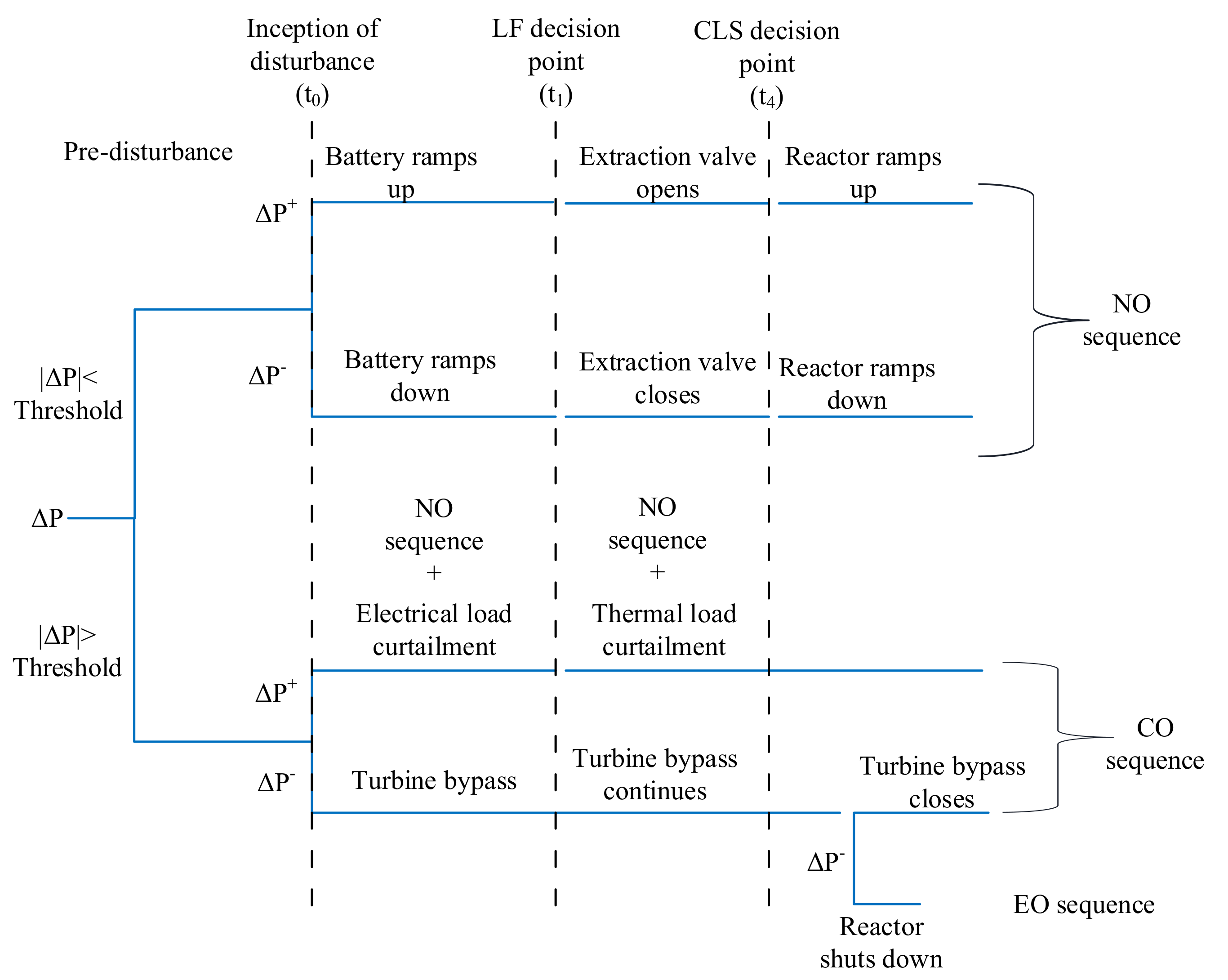
3.3. Resilience Framework

Any disturbance in a power system will require either an increase or decrease in power as a response from generation assets. For the purposes of this paper, the events requiring power increase are referred to as $\Delta P^{+}$, and the events requiring power decrease are referred to as $\Delta P^{-}$. In the proposed resilience framework, the real-power flexibility of microgrid assets is evaluated and aggregated to obtain overall adaptive capacity of a microgrid to respond to $\Delta P^{+}$ and $\Delta P^{-}$. Note that the proposed framework does not evaluate the microgrid’s response against the classes of disturbances or the performance of the microgrid following a disturbance. Instead, it identifies the adaptive capacity of the microgrid to respond to generation–demand imbalance created by any means, including large disruptive events and DER generation uncertainty.

The resilience framework is developed for the SMR-DER integrated-energy microgrid considering two operating scenarios: normal operation (NO) and compromised operation (CO). The NO includes operating conditions when the flexibility needs of a microgrid can be fulfilled by controlling assets normally based on the operational framework described in Section 3.1. The CO refers to abnormal operating conditions when NO of assets does not meet the flexibility needs of the microgrid, and additional flexibility schemes are activated.

During NO, the disturbances are typically smaller such that the assets operating normally will be able to handle them. BES alone can respond to immediate real-power imbalance without compromising the dynamic performance. Once the system reaches the start of the next LF cycle (i.e., LF decision point), steam extraction system provides additional flexibility. Once the system reaches the start of the next CLS cycle (i.e., CLS decision point), further flexibility will be added by the reactor’s power maneuvering capability. The steam extraction system will be able to provide maximum LF response as long as the TES temperature is within minimum and maximum limits. The SOC levels of TES and BES are important factors to meet the flexibility requirement of a system against disturbances that last longer in the system. In NO, the reactor must comply with the ramp rate and total power change limits, as given by (11) and (12), respectively.

Figure 5 illustrates the asset operation following the disturbance during NO along with flexibility limits for different assets in the system. Note that the figure is just an illustration and does not reflect the time and sequence of asset activation and the magnitude of variables in scale. The time of asset activation and the system adaptive capacity depends on the system’s dynamic state at the onset of a disturbance.

Figure 6 shows the activation of additional flexibility during CO. During CO, the system would be prioritized to meet the demands of critical loads. For $\Delta P^{+}$, additional flexibility is added by curtailing non-critical electrical loads which can be activated immediately following a disturbance. Curtailing thermal loads would also be useful if the SOC level of the TES drops below the minimum limit. For $\Delta P^{-}$, the turbine bypass system can bypass excess steam to the condenser. The condenser can receive 100% of the process steam but only for a limited time. Once the system reaches the LF decision point, further flexibility could be added with curtailable thermal loads. Because the extraction steam has much less enthalpy compared to the directly bypassed steam, the full steam extraction capability can be used as long as needed. In other words, the maximum amount of steam that can be extracted to the heating side in response to $\Delta P^{-}$ is not limited by the TES SOC. During CO, unlike during NO, the reactor power level of SMR can be maneuvered up to its maximum or minimum limits irrespective of the power change limit given by (12).

In the case of $\Delta P^{-}$, if the generation–demand imbalance sustains even after continuous bypassing of steam for a certain allowed duration, the reactor will isolate from the microgrid and initiate emergency shutdown. This operating event is termed as emergency operation (EO) which arises due to large disturbances, such as sustained faults and total loss of electrical connection of SMR to microgrid. The EO is an event that originates out of CO rather than a separate operational mode. The $\Delta P^{+}$, on the other hand, may force the system to compromise the power supply to critical loads but not the reactor safety itself.

The event tree in Figure 7 shows the decision-making process following a disturbance. Based on the magnitude and form of the disturbance, the microgrid activates its flexible assets to respond to the generation–demand imbalance created. The microgrid switches between these operating modes in real time to respond to power fluctuation created by the disturbance. The seamless transition between the operational modes in real time is crucial. At the onset of disturbance, BES starts responding with the system assuming NO. If BES is unable to meet generation–demand balance, additional assets such as turbine bypass system or load curtailment activate switching system from NO to CO. If the disturbance dies out sooner, the system will first withdraw the assets that were activated as a part of CO followed by the assets of NO. In this way, the system will smoothly transition between NO and CO. Based on temporal characteristics of the disturbance, the system can switch between CO and NO at any time. To facilitate this seamless transition, the assets are decoupled to not disrupt the operational pattern of one another. For example, switching to CO does not allow the system to operate steam extraction or reactor control before the decision point. Rather, an equivalent change is achieved by other independent methods such as turbine bypass system or load curtailments. This allows operation at pre-optimized setpoints following the return of the system to NO after the disturbance dies out. Once the reactor shutdown sequence (EO mode) is activated, the system will not be able to recover. The microgrid should therefore continue operating in CO mode long enough to evaluate if the switching to EO mode is absolutely necessary.

In the proposed resilience model, the asset-level flexibility shown in Figure 5 and Figure 6 are aggregated to obtain the adaptive real-power capacity of the microgrid in NO and CO mode. The adaptive capacity evaluated in NO and CO modes are analyzed to identify the disturbance threshold for microgrid control to facilitate quicker and efficient decision-making. Based on this threshold measurement, the microgrid selects between NO or CO mode, as shown in Figure 7. In actual operation, the resilience information obtained in real time can also be used to supervise the microgrid management system to reconfigure its assets to maximize operational resilience.

4. Case Study

A microgrid system is developed in a portion of the IEEE-30 bus network hosting generation in the form of an SMR plant and renewables. The district heating (DH) system is also integrated into the SMR plant. First, the case system is discussed along with the simulation results which include the 720 h quasi-static simulation and a 2.5 h dynamic simulation. The result is then shown in analyzing the microgrid’s operational resilience in terms of adaptive real-power capacity for normal, compromised, and emergency operations. Note that the microgrid model and the operation simulation in this case study are replicated from [20]. Readers are highly encouraged to refer to [20,21] for background details on the case system and operational setup. In this paper, the system details and operational simulation results are summarized before moving into the resilience evaluation part.

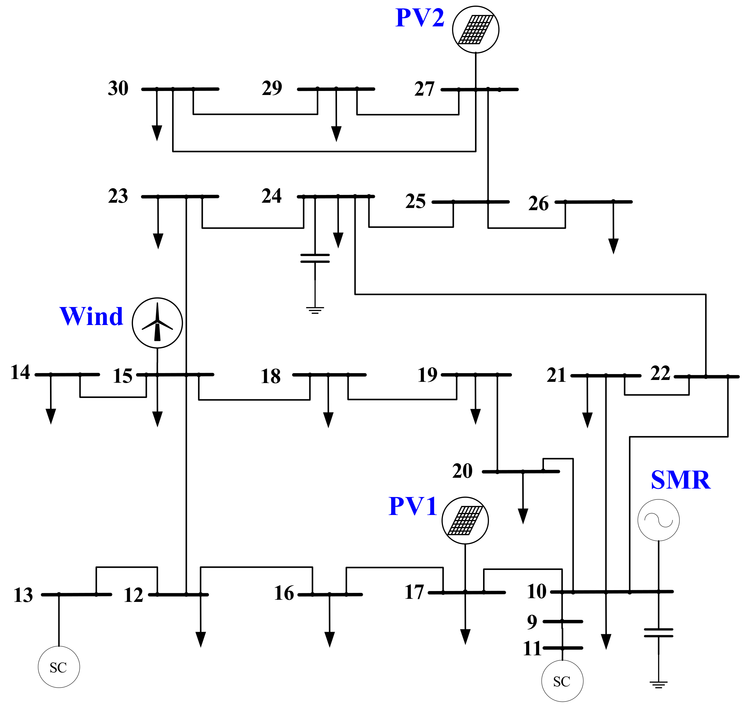
4.1. Modified IEEE-30 Bus System

The IEEE-30 bus system consists of 33 kV and 230 kV transmission network [48]. The 33 kV portion can be isolated from the 230 kV system by taking four 230/33 kV transformers out of service. The resulting 33 kV network is used as a case system to develop the microgrid model for this paper. Figure 8 shows the proposed case system which has total electrical load of 102 MWe. The proposed case system does not have any generation source. Therefore, to meet the system demand, new power generation sources are needed. A microgrid with a cogenerating SMR plant, wind, PV, BES, and TES is suitable for the system. An SMR plant with two NuScale integral pressurized-water reactor (iPWR)-type SMRs, rated 50 MWe each, is hosted at node 10. A wind plant, sized 30 MWe, is hosted at node 15, and two PV plants, 10 MWe each, are hosted at node 17 and node 27, respectively. A centralized BES is hosted at node 10 to support SMR for short-term response. The system also has two synchronous condensers (SC) at nodes 11 and 13 to provide reactive power support.

The DH system is sized based on the size of electrical system and lumped as a single load. The TES is collocated with the SMR plant along with HXs, as shown in Figure 3. Reference [21] provides the optimum sizing of generation assets based on operational and economic constraints including reactor maneuvering limits, heat waste in DH system, cost of BES, and power system dynamic performance. The sizing of assets is summarized in

Table 1. Microgrid design parameters.

Microgrid Assets		Parameters
System Level		$t_{CLS}$ = 6 h, $t_{LF}$ = 15 min,
		$P_{max}^{curt}$ = 0.25 of $P_t^D$, $Q_{max}^{curt}$ = 0.25 of $Q_t^D$
SMR Plant	Reactor	$N_R$ =2, $t_R$ = 2 h, $t_H$ = 4 h, $P_{max}^{R,e}$ = 50 MWe,
		$P_{min}^{R,e}$ = 7.82 MWe, $P_{max}^{R,th}$ = 160 MWt,
		$P_{min}^{R,th}$ = 32 MWt, ${\dot{m}}_{rat}^{SG}$ = 65.93 kg/s, $\Delta P_{max}^{R,th}$ = 0.3 pu,
		$R_{th}^D$ = −0.15 pu/h, $R_{th}^U$ = 0.15 pu/h
	Steam Extraction	$T_{ext}$ = 128 ${}^{\circ }$C
	Turbine Bypass	$\Delta f_{set}$ = 0.1 Hz, $t_{max}^{BV}$ = 2*$t_{LF}$ = 30 min,
		$R_{BV}^D$ = −1.32 kg/s2, $R_{BV}^U$ = 1.32 kg/s2
DH system		${\dot{m}}_{max}^{HX1}$ = ${\dot{m}}_{max}^{HX2}$ = 50 kg/s; $v_{str}$ = 20,000 m3;
		$T_{min}^{str}$ = 70 ${}^{\circ }$C; $T_{max}^{str}$ = 98 ${}^{\circ }$C; $c_p$ = 4.18 kJ/kg ${}^{\circ }$C;
		$T_{rat}^{DHout}$ = 90 ${}^{\circ }$C; $T_{min}^{DHout}$ = 70 ${}^{\circ }$C
BES		$P_{max}^B$ = 10 MWe, $P_{min}^B$ = −10 MWe, $E_{rat}^B$ = 10 MWeh,
		$E_{max}^B$ = 0.95 pu, $E_{min}^B$ = 0.25 pu
		$R_{BV}^D$ = −0.5 MW/s, $R_{BV}^U$ = 0.5 MW/s
Wind		$N_{WT}$ = 20; $P_r^w$ = 1.5 MWe; ${\omega }_{ci}$ = 14.4 km/h;
		${\omega }_r$ = 37 km/h; ${\omega }_{co}$ = 90 km/h
PV		${\eta }_p$ =16%; $A_p$ = 109,649.1 m2

. The loads centers in Figure 8 are populated with residential, industrial, and commercial load profiles of 15 min resolution obtained from [49]. The heat demand profile is obtained by scaling practical heat load profile from [50] with 15 min resolution. The wind and PV generation profiles are obtained from [51,52,53], respectively.

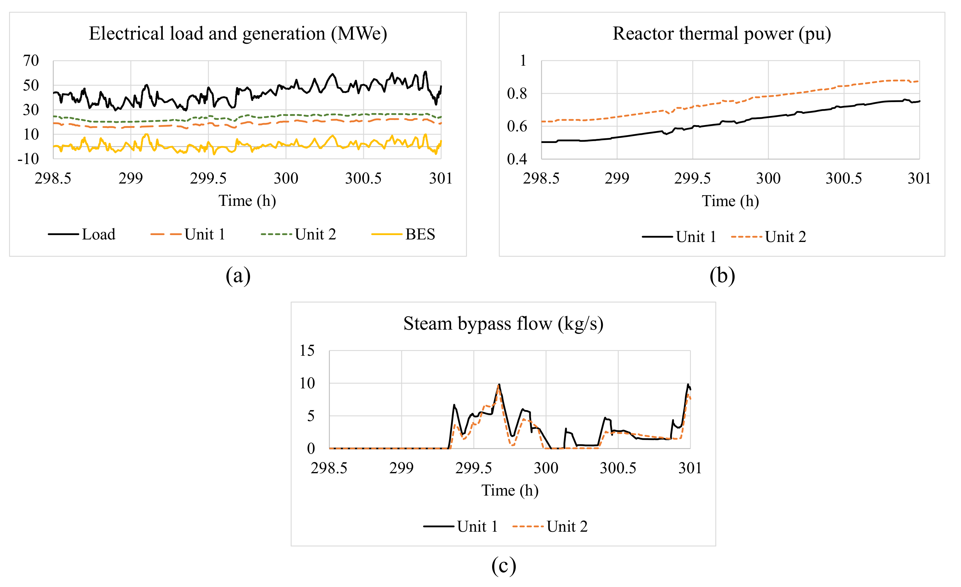
4.2. Operational Results

In this paper, the operational simulation in [21] is replicated with the resilience framework functionality integrated in the microgrid model. In this paper, the resilience model is used for system observation rather than to execute any control actions. Therefore, the operational results will be identical to the ones in [21]. The description below will focus only on results essential for the resilience evaluation. The quasi-static simulation is performed for a month with a 15 min simulation timestep. The case system of Figure 8 developed in Power System Simulator Siemens Network Calculation (PSS/Sincal) [54] is cosimulated with the quasi-static model of SMR units and DH system developed in MATLAB. It captures the CLS and LF controls of the microgrid. The dynamic simulation is performed in Power System Simulator for Engineering (PSS/E) [55] for the 2.5 h period which contains the largest fluctuations in the system to analyze FC control and its interaction with CLS and LF controls.

Figure 9 shows the results of quasi-static simulation. The electrical load variations along with the intermittency of wind and PV are the source of fluctuations on the electrical side. Figure 9a shows the demand at the SMR bus (Bus 10) which is taken as the slack bus for power flow simulations. On a daily basis, the PV generation goes through zero-power output periods during the nighttime. During the daytime, the PV generation faces large fluctuations due to the cloud movement covering the direct irradiance to the solar panels. Similarly, the wind power fluctuates based on the wind speed. The power outputs of wind and PV plants vary as high as 47% and 61%, respectively, of their rated output within a minute. This integration of wind and PV generation results in large power fluctuations in the microgrid which are managed by controlling the power outputs of flexible assets. As discussed earlier, the reactor power is controlled a fixed number of times per day based on the CLS algorithm. In the proposed scheme, usually only one unit is controlled in a CLS interval while another one remains on hold to reduce the total number of reactor power maneuvers. Out of the 120 CLS intervals, both units were required to provide power maneuvering on one occasion to meet large demand fluctuations. Similarly, for three CLS intervals, none of the units were required to change their power levels. Figure 9c shows the reactor power level for the two units over the 720 h duration that included 120 CLS intervals and total of 116 reactor power maneuvers.

Figure 9b shows DH steam extraction as a ratio of the total steam generated and the SMR plant’s instantaneous electrical power in per unit (pu) of its rated electrical output. As seen in Figure 9a,b, when the power output from wind and PV plants increases, SMR’s demand decreases. In response, the extraction flow to the DH system is increased to reduce the electrical output of SMR. The extraction steam is utilized to meet the heating demands with TES absorbing the surplus steam or supplying the deficient heat to the DH pipeline. Due to this, the TES temperature fluctuates during the simulation as shown in Figure 9d. For 2.4% of time, the TES was at upper limit and was not able to accept surplus steam, and the extraction steam excess to the DH system was directly bypassed to the condensor. The DH temperature never went below the lower limit and was always able to supply the deficient heat to the DH pipeline when the steam extracted was not sufficient to fulfill the DH demand.

In quasi-static simulation, BES and turbine bypass valves remain inactive, as they are operated to provide primary response to the frequency deviations. The quasi-static simulation only shows the CLS and LF controls. It does not account for the smaller fluctuations present within each LF intervals that occur due to short-term wind and PV intermittency.

The dynamic simulation is performed for a 2.5 h time segment of quasi-static simulation which includes largest fluctuations from quasi-static simulation (i.e., between 298.5 to 301 h). This 2.5 h period includes the reactor ramping period of the CLS control. Both reactor units were ramped up between 298.75 to 300.75 h as shown in Figure 10b. It also includes 10 consecutive LF controls which are repeated in the intervals of 15 min. Figure 10a plots the electrical power outputs of the two SMR units along with the load demand and BES power output. BES is operated to respond to the frequency deviation occurring due to generation–demand imbalance persisting after the CLS and LF control. When BES alone is not able to meet the FC requirements, the turbine bypass system operates as shown in Figure 10c.

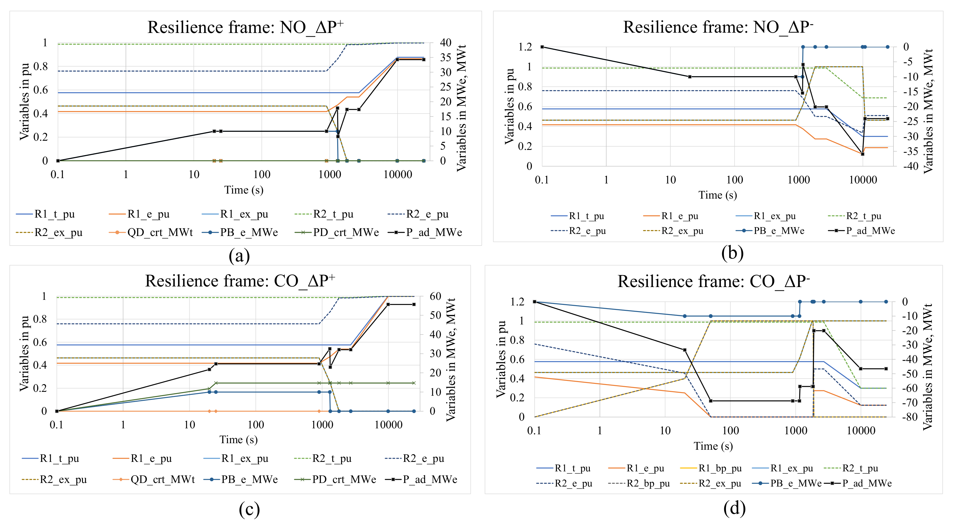
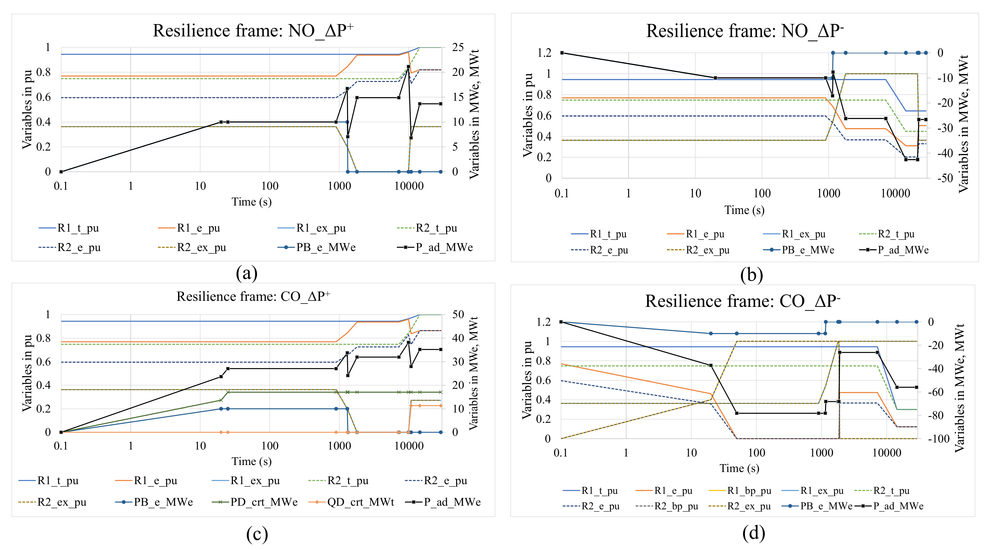
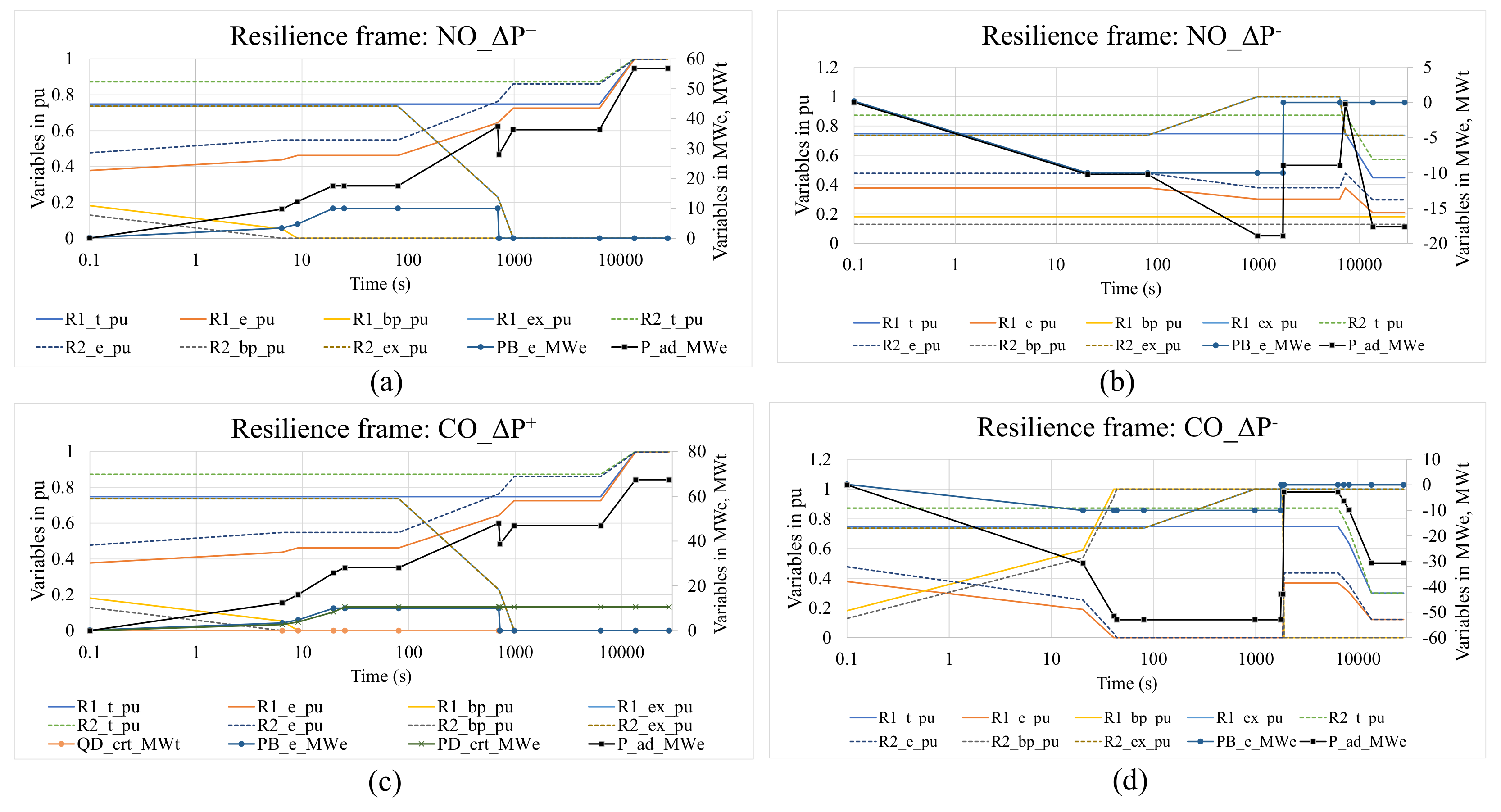
4.3. Resilience Evaluation

The resilience model takes system dynamic states as inputs and analyzes the asset’s capabilities at each simulation timestep. Looking forward in time, the magnitude and temporal constraints of microgrid assets are analyzed to obtain the flexibility characteristics that provide the magnitude shape of the real-power variation they can offer for a certain amount of time. These flexibility characteristics of assets are then aggregated to obtain the overall adaptive capacity characteristics of the microgrid.

The graph showing the temporal characteristics of asset-level flexibility and overall adaptive capacity is referred to as the resilience frame. Resilience frames are generated in real time at each simulation timestep. The time axis of a resilience frame begins at 0 s, corresponding to the simulation time at which resilience is being analyzed, and lasts until the end of subsequent CLS interval, assuming no substantial flexibility can be added after CLS is executed. Note that the resilience frame is an exploration of a future response to predict the adaptive capacity of microgrid in real time at each simulation timestep. The time axis of resilience frame is not a part of the actual operational simulation being executed.

Logarithmic scale is used for time axes of the resilience frame to illustrate the roles of different assets that differ significantly in terms of their activation and operation times. For example, BES can ramp up to maximum power in either direction within 20 s, whereas steam extraction system takes 15 min and reactor ramping takes 2 h. Logarithmic scale adequately represents operation of assets with significantly different temporal characteristics in a single graph.

The resilience model is integrated into both quasi-static and dynamic simulation models of the microgrid. Sample calculations are shown for three different cases: two for quasi-static simulation and one for dynamic simulation. The system resilience is then quantified in terms of the normalized area under the adaptive capacity curve, termed as RAM, for both NO and CO modes. The $\Delta P^{+}$ and $\Delta P^{-}$ flexibilities are analyzed separately for each operational mode. Note that the proposed resilience model calculates the maximum adaptive capacity instead of analyzing the response to a disturbance. Therefore, the asset will be operated up to their limits allowed in each operational mode.

Table 2. Description of variables plotted in Figure 11, Figure 12 and Figure 13.

Variable	Description
Rx_t_pu, x = 1,2	Reactor thermal power level of unit x in pu
Rx_e_pu, x = 1,2	Reactor electrical power level of unit x in pu
Rx_ex_pu, x = 1,2	Extraction steam flow rate of unit x in pu
Rx_bp_pu, x = 1,2	Bypass steam flow rate of unit x in pu
PB_e_MWe	Battery electrical power output in MWe
PD_crt_MWe	Electrical load curtailed in MWe
QD_crt_MWt	Thermal load curtailed in MWt
P_ad_MWe	Microgrid adaptive real-power capacity in MWe

provides the description of variables shown in the resilience frames in Figure 11, Figure 12 and Figure 13.

The first case selected is 0 h of the simulation. At 0 h, TES is at 90 ${}^{\circ }$C, and BES SOC is at 0.65 pu. Figure 11a–d shows the resilience frames for four cases: $\Delta P^{+}$ and $\Delta P^{-}$ for NO and CO. The flexibility offered by different assets and their aggregated, in terms of the adaptive real-power capacity changing with time, are shown in each resilience frame. The BES starts ramping up or down immediately and lasts until it reaches its upper or lower SOC limits (given in Table 1). For $\Delta P^{+}$, after BES reaches its lower SOC limit, it can no longer discharge, and BES power returns to zero at 1306 s, shown in Figure 11a,c. Similarly, for $\Delta P^{-}$, BES power returns to zero after reaching the upper SOC limit at 1144 s, shown in Figure 11b,d. The LF decision point arrives at 900 s, and the CLS decision point arrives at 2700 s. At the LF decision point, the steam extraction valves can be controlled to their limits in either direction (i.e., completely closed extraction valve or 0 kg/s extraction for $\Delta P^{-}$) and completely open extraction valve or full ${\dot{m}}_t^{SG}$ extraction for $\Delta P^{-}$. Similarly, both reactor units are allowed to maneuver at once but up to the reactor power change limits (see Table 1). The reactor power ramping completes at 9900 s, and the reactor stays on hold until the next CLS decision point at 24,300 s. The TES did not fully discharge over the duration considered, and, therefore, the flexibility offered by the steam extraction for $\Delta P^{+}$ remained over the resilience frame.

For $\Delta P^{+}$ in CO, the non-critical electrical loads were curtailed immediately to meet the short-term response. For $\Delta P^{-}$ in CO, the turbine bypass system operates which brings electrical power output of SMRs to zero, as shown in Figure 11d. After two LF cycles, the turbine bypass system is withdrawn. This significantly reduces the adaptive capacity in CO mode. Although not analyzed in this paper, if a power imbalance persists even after bypassing of steam for two LF cycles, the reactor will initiate the emergency shutdown. For $\Delta P^{-}$ in CO, the steam extraction can be fully operated irrespective of the TES temperature limits as the excess low-temperature extracted steam can be continuously bypassed to the condenser.

The second case is for 216.75 h of the simulation, as shown in Figure 12a–d. Similar to the first case, the BES is activated immediately for NO, and electrical load curtailment or turbine bypass system are activated for CO mode. Steam extraction system and reactor maneuvering both started at 900 s after the disturbance. Initially, BES SOC was 0.65 pu, and the TES temperature was 74.15 ${}^{\circ }$C. This case with low starting TES temperature is selected to demonstrate how the quick depletion of TES SOC will impact the operational resilience on the power side. In this case, the TES temperature reaches its lower limit of 70 ${}^{\circ }$C at 9900 s. After TES reached its lower temperature, the steam extraction system could not provide LF control for $\Delta P^{+}$ in NO mode. This results in sharp reduction of adaptive real-power capacity at 9900 s, as shown in Figure 12a. For $\Delta P^{+}$ in CO mode, the non-critical thermal load is curtailed to provide additional flexibility on the electrical side, as shown in Figure 12b. All other results are similar to the first case.

The third case shown in Figure 13a–d is for 300.97769 h of the simulation where the resilience model uses system state values directly from dynamic simulation. Initially, BES SOC was at 0.463 pu and TES at 92.72 ${}^{\circ }$C. Compared to the second case, BES discharged quicker for $\Delta P^{+}$. Similarly, the bypass valve flows were non-zero at the start: 0.182 pu/s (i.e., 12.11 kg/s) for unit 1 and 0.129 pu/s (i.e., 8.59 kg/s) for unit 2. For $\Delta P^{+}$, the bypass flows came back to zero, as shown in Figure 13a,c, whereas for $\Delta P^{-}$, the bypass flows stayed at the initial non-zero value for NO, as shown in Figure 13b. For $\Delta P^{-}$ in CO, the bypass flows ramp up to maximum, as shown in Figure 13d. All other results are similar to the earlier two cases.

Figure 11, Figure 12 and Figure 13 show the use of proposed resilience frame to evaluate system adaptive real-power capacity. These three cases show that the resilience model can be used with both quasi-static and dynamic simulations. The adaptive real-power capacity changes over time due to ramping delays of the assets, activation delays of new assets, and exhaustion of energy-limited assets. The adaptive capacity curves produced in Figure 11, Figure 12 and Figure 13 give an idea of the disturbance characteristics the microgrid can respond to in different modes of operation.

Figure 14 maps the adaptive capacity curve to the DIRE curve for the first case of 0 h to analyze the Rs of resilience (i.e., resist, response, and recover). Although all assets are represented in terms of their capacity to respond to disturbances, they have different principal functions. BES, for example, is operated immediately and helps to arrest disturbance and resist the dynamic performance degradation. Therefore, a part of the BES response will fall under the resist epoch which is considered in the first 10 s of the resilience frame for the purpose of this paper. It is the time when a disturbance typically grows. The steam extraction system operates to maintain generation–demand balance for steady-state operation. It falls mainly during the response epoch between 10–1000 s during which disturbance reaches its peak and persists. The reactor power control with CLS falls under recover epoch (>1000 s), and it helps recover steam extraction setpoint and energy lost of energy-limited assets while responding to the disturbance.

As discussed earlier, the adaptive capacity is a temporal characteristic rather than a single point value. Therefore, it is not computationally viable to analyze the whole characteristics in real-time decision-making. To compare the system resilience over time, a metric is introduced quantifying the temporal change of adaptive real-power capacity with a single variable. The metric termed as RAM is given as

$$RAM=\frac{\mathrm{Area}\mathrm{under}\mathrm{adaptive}\mathrm{capacity}\mathrm{curve}}{\mathrm{Total}\mathrm{duration}}=\frac{{\int }_0^{t_{FF}}P\text{\_}ad\text{\_}MWe}{t_{FF}}\mathrm{MWe}\text{-}\mathrm{s}/\mathrm{s}$$

(32)

where $P\text{\_}ad\text{\_}MWe$ is time-varying system adaptive capacity as obtained from the resilience frame, and $t_{FF}$ is the total duration of the resilience frame.

RAM represents the average adaptive capacity over the resilience time frame. RAM evaluated for simulation period 0 h to 720 h is plotted in Figure 15. It includes RAM values for each quasi-static simulation time steps and 2.5 h dynamic simulation period. The RAM values for the 2.5 h dynamic simulation are plotted in the zoomed section in Figure 15b.

The RAM values provide information to the system regarding its capacity to respond to any disturbance that may arise. Figure 15a,b shows the calculation of RAM values in real time, parallel to the simulation. This information can be provided as a feedback to the microgrid management system in real time to execute precautionary actions such as reconfiguration of assets to improve operational resilience. Figure 15 clearly shows that the resilience values are inconsistent over simulation duration. For example, the RAM values in NO for $\Delta P^{+}$ reached its lowest of 6.05 MWe at 258.75 h, whereas for $\Delta P^{-}$, it was −6.56 MWe at 300.9656 h. If the system were to face disturbances larger than these values, it may have to switch to CO. In CO, RAM was a minimum of 28.92 MWe at 258.75 h for $\Delta P^{+}$ and −13.99 MWe for $\Delta P^{+}$ at 298.7347 h.

Although RAM provides high-level information on system resilience as discussed, it has some limitations. Firstly, it does not properly credit the contributions of short-term assets. The short-term assets such as BES will not have a large area contribution to the RAM due to energy limitation, but they are crucial to arrest the disturbance immediately after its inception. Secondly, RAM also loses the temporal feature of adaptive capacity curve which is crucial to analyze dynamic characteristics of disturbances. Therefore, in this paper, we intend to present RAM as a comparison metric for studies and an initial guidance for metric development rather than a final product. The next steps are to resolve these limitations of the RAM model, identify standard limits for RAM for comparison in real-time operation, and develop control algorithms for microgrid to take precautionary actions based on RAM feedbacks.

5. Conclusions and Future Work

Amid increasing interest in SMR use in microgrids, this paper analyzed SMR salient features and modeled the interaction between heat and power systems to develop a framework that evaluates adaptive capacity for the resilient operation of SMR-DER integrated-energy microgrids. An operational scheme is designed for microgrid control that decoupled overall microgrid operation into three separate controls of CLS, LF, and FC. In addition to normal operation, operational algorithms were discussed for CO. The proposed resilience model aggregates asset-level real-power flexibility to evaluate the operational resilience indicator in terms of adaptive real-power capacity characteristics. The adaptive capacity curve produced has both time and magnitude characteristics which reflect the operational margin of the system to respond to generation–demand imbalance created by any form of disturbances, including large disruptive events and generation uncertainties. A single point operational metric known as RAM was also obtained from the adaptive capacity characteristic to compare the operational resilience over time and provide high-level guidance to microgrid operators. The quasi-static simulation results for 720 h and the dynamic simulation results for 2.5 h show that the system with the proposed operational framework is resilient enough to withstand and operate normally with DER penetration level as high as 50% (50 MWe, wind, and PV collectively). The RAM results shown reflect the system resilience in real time while operating with the proposed operational framework. The case study clearly shows that the proposed resilience model can improve the operational awareness of the microgrid and help optimize the system control.

The adaptive capacity framework, previously limited to resilience modeling of power system components, is extended in this paper to characterize the impact of nuclear and heating systems on overall system resilience. The proposed model improves the awareness of power side to the nuclear and heating sides and vice versa for resilience planning, operational decision-making, and real-time control. Future work planned with this resilience framework includes incorporating the inertial response as a part of the resist epoch, including more detailed operational procedure of SMRs based on data from manufacturers and operators, including curtailment models of wind and PVs to support resilience, synthetic inertia by inverter-based resources in microgrids, and analyzing the reactive power capabilities of system assets. Further work is necessary to resolve the limitations with the RAM model and develop its standards. Future work will also demonstrate the application of the proposed metric for real-time system control with hardware-in-loop or software-in-loop simulations.

References

1. Brundtland, G. Report of the World Commision on Environement and Development: Our Common Future; Oxford Paperbacks: Oxford, UK, 1987. [Google Scholar]
2. Kenward, A.; Raja, U. Blackout: Extreme Weather, Climate Change and Power Outages; Technical Report; Climate Central: Princeton, NJ, USA, 2014. [Google Scholar]
3. U.S. Department of Energy Office of Electricity Delivery and Energy Reliability. Economic Benefits of Increasing Electric Grid Resilience to Weather Outages; Technical Report; Executive Office of the President: Washington, DC, USA, 2013.
4. Busby, J.W.; Baker, K.; Bazilian, M.D.; Gilbert, A.Q.; Grubert, E.; Rai, V.; Rhodes, J.D.; Shidore, S.; Smith, C.A.; Webber, M.E. Cascading risks: Understanding the 2021 winter blackout in Texas. Energy Res. Soc. Sci. 2021, 77, 102106. [Google Scholar] [CrossRef]
5. Panteli, M.; Mancarella, P. The grid: Stronger, bigger, smarter?: Presenting a conceptual framework of power system resilience. IEEE Power Energy Mag. 2015, 13, 58–66. [Google Scholar] [CrossRef]
6. McJunkin, T.R.; Reilly, J.T. Net-Zero Carbon Microgrids; Technical Report INL/ EXT-21-65125; Idaho National Laboratory: Idaho Falls, ID, USA, 2021. [Google Scholar] [CrossRef]
7. International Atomic Energy Agency. Advances in Small Modular Reactor Technology Developments: A Supplement to IAEA Advanced Reactors Information System (ARIS); IAEA: Vienna, Austria, 2016; p. 400. [Google Scholar]
8. Poudel, B.; McJunkin, T.R.; Kang, N.; Reilly, J.T. Small Reactors in Microgrids: Technical Studies Guidance; Technical Report INL/EXT-21-64616-Rev000; Idaho National Laboratory: Idaho Falls, ID, USA, 2021. [Google Scholar] [CrossRef]
9. Kennedy, J.C.; Bragg-sitton, S.; Mcclure, P. Special Purpose Application Reactors: Systems Integration Decision Support; Technical Report INL/ EXT-18-52369; Idaho National Laboratory: Idaho Falls, ID, USA, 2018. [Google Scholar]
10. Islam, M.R.; Gabbar, H.A. Study of small modular reactors in modern microgrids. Int. Trans. Electr. Energy Syst. 2015, 25, 1943–1951. [Google Scholar] [CrossRef]
11. Ingersoll, D.T.; Colbert, C.; Houghton, Z.; Snuggerud, R.; Gaston, J.W.; Empey, M. Can Nuclear Power and Renewables be Friends? In Proceedings of the International Congress on Advances in Nuclear Power Plants (ICAPP), Nice, France, 3–6 May 2015; p. 9. [Google Scholar]
12. Joshi, K.; Poudel, B.; Gokaraju, R.R. Investigating small modular reactor’s design limits for its flexible operation with photovoltaic generation in microcommunities. J. Nucl. Eng. Radiat. Sci. 2021, 7, 1–10. [Google Scholar] [CrossRef]
13. Joshi, K.A.; Poudel, B.; Gokaraju, R. Exploring synergy among new generation technologies-small modular reactor, energy storage, and distributed generation: A strong case for remote communities. J. Nucl. Eng. Radiat. Sci. 2020, 6, 1–9. [Google Scholar] [CrossRef] [Green Version]
14. Ingersoll, D.T.; Colbert, C.; Bromm, R.; Houghton, Z. NuScale Energy Supply for Oil Recovery and Refining Applications. In Proceedings of the International Congress on Advances in Nuclear Power Plants (ICAPP), Charlotte, NC, USA, 6–9 April 2014; pp. 2344–2351. [Google Scholar]
15. Ingersoll, D.T.; Houghton, Z.J.; Bromm, R.; Desportes, C. NuScale small modular reactor for Co-generation of electricity and water. Desalination 2014, 340, 84–93. [Google Scholar] [CrossRef]
16. Lindroos, T.J.; Pursiheimo, E.; Sahlberg, V.; Tulkki, V. A techno-economic assessment of NuScale and DHR-400 reactors in a district heating and cooling grid. Energy Sources Part B Econ. Plan. Policy 2019, 14, 13–24. [Google Scholar] [CrossRef]
17. Värri, K.; Syri, S. The Possible Role of Modular Nuclear Reactors in District Heating: Case Helsinki Region. Energies 2019, 12, 2195. [Google Scholar] [CrossRef] [Green Version]
18. International Atomic Energy Agency. Opportunities for Cogeneration with Nucelar Energy; Technical Report NP-T-4.1; IAEA Nuclear Energy Series: Vienna, Austria, 2013. [Google Scholar]
19. Locatelli, G.; Boarin, S.; Fiordaliso, A.; Ricotti, M.E. Load following of Small Modular Reactors (SMR) by cogeneration of hydrogen: A techno-economic analysis. Energy 2018, 148, 494–505. [Google Scholar] [CrossRef]
20. Poudel, B.; Gokaraju, R. Small Modular Reactor (SMR) Based Hybrid Energy System for Electricity and District Heating. IEEE Trans. Energy Convers. 2021, 36, 2794–2802. [Google Scholar] [CrossRef]
21. Poudel, B.; Gokaraju, R. Optimal Operation of SMR-RES Hybrid Energy System for Electricity and District Heating. IEEE Trans. Energy Convers. 2021, 36, 3146–3155. [Google Scholar] [CrossRef]
22. Panteli, M.; Trakas, D.N.; Mancarella, P.; Hatziargyriou, N.D. Power Systems Resilience Assessment: Hardening and Smart Operational Enhancement Strategies. Proc. IEEE 2017, 105, 1202–1213. [Google Scholar] [CrossRef] [Green Version]
23. Holling, C.S. Resilience and stability of ecological systems. Annu. Rev. Ecol. Syst. 1973, 4, 1–23. [Google Scholar] [CrossRef] [Green Version]
24. Tierney, K.; Bruneau, M. Conceptualizing and Measuring Resilience: A Key to Disaster Loss Reduction. In TR News; Transportation Research Board: Washington, DC, USA, 2007; pp. 14–18. [Google Scholar]
25. Paolo, G.; Reinhorn, A.M.; Bruneau, M. Framework for analytical quantification of disaster resilience. Eng. Struct. 2010, 32, 3639–3649. [Google Scholar] [CrossRef]
26. Ouyang, M.; Dueñas-osorio, L.; Min, X. A three-stage resilience analysis framework for urban infrastructure systems. Struct. Saf. 2012, 36–37, 23–31. [Google Scholar] [CrossRef]
27. Ouyang, M.; Dueñas-osorio, L. Multi-dimensional hurricane resilience assessment of electric power systems. Struct. Saf. 2014, 48, 15–24. [Google Scholar] [CrossRef]
28. Panteli, M.; Trakas, D.N.; Mancarella, P.; Hatziargyriou, N.D. Boosting the Power Grid Resilience to Extreme Weather Events Using Defensive Islanding. IEEE Trans. Smart Grid 2016, 7, 2913–2922. [Google Scholar] [CrossRef]
29. McJunkin, T.R.; Rieger, C.G. Electricity distribution system resilient control system metrics. In Proceedings of the 2017 Resilience Week, RWS 2017, Wilmington, DE, USA, 18–22 September 2017; pp. 103–112. [Google Scholar] [CrossRef]
30. Hovland, K.A.; Gentle, J.P.; Morash, S.; Placer, N. Resilience Framework for Electric Energy Delivery Systems; Technical Report INL/EXT-21-62326, Rev 1; Idaho Falls: Idaho, ID, USA, 2021. [Google Scholar]
31. Bagchi, S.; Aggarwal, V.; Chaterji, S.; Douglis, F.; Gamal, A.E.; Han, J.; Henz, B.J.; Hoffmann, H.; Jana, S.; Kulkarni, M.; et al. Vision Paper: Grand Challenges in Resilience: Autonomous System Resilience through Design and Runtime Measures. IEEE Open J. Comput. Soc. 2020, 1, 155–172. [Google Scholar] [CrossRef]
32. Panteli, M.; Mancarella, P. Influence of extreme weather and climate change on the resilience of power systems: Impacts and possible mitigation strategies. Electr. Power Syst. Res. 2015, 127, 259–270. [Google Scholar] [CrossRef]
33. Chanda, S.; Srivastava, A.K.; Mohanpurkar, M.U.; Hovsapian, R. Quantifying Power Distribution System Resiliency Using Code-Based Metric. IEEE Trans. Ind. Appl. 2018, 54, 3676–3686. [Google Scholar] [CrossRef]
34. Rieger, C.G. Resilient control systems Practical metrics basis for defining mission impact. In Proceedings of the 7th International Symposium on Resilient Control Systems, ISRCS 2014, Denver, CO, USA, 19–21 August 2014. [Google Scholar]
35. Eshghi, K.; Johnson, B.K.; Rieger, C.G. Power system protection and resilient metrics. In Proceedings of the 2015 Resilience Week, RWS 2015, Philadelphia, PA, USA, 18–20 August 2015; pp. 212–219. [Google Scholar] [CrossRef]
36. Phillips, T.; McJunkin, T.; Rieger, C.; Gardner, J.; Mehrpouyan, H. An Operational Resilience Metric for Modern Power Distribution Systems. In Proceedings of the 2020 IEEE 20th International Conference on Software Quality, Reliability, and Security Companion, QRS-C 2020, Macau, China, 11–14 December 2020; pp. 334–342. [Google Scholar] [CrossRef]
37. Phillips, T.; Chalishazar, V.; McJunkin, T.; Maharjan, M.; Shafiul Alam, S.M.; Mosier, T.; Somani, A. A metric framework for evaluating the resilience contribution of hydropower to the grid. In Proceedings of the 2020 Resilience Week, RWS 2020, Salt Lake City, UT, USA, 19–23 October 2020; pp. 78–85. [Google Scholar] [CrossRef]
38. Phillips, T.; McJunkin, T.; Rieger, C.; Gardner, J.; Mehrpouyan, H. A framework for evaluating the resilience contribution of solar PV and battery storage on the grid. In Proceedings of the 2020 Resilience Week, RWS 2020, Salt Lake City, UT, USA, 19–23 October 2020; pp. 133–139. [Google Scholar] [CrossRef]
39. Kundur, P. Power System Stability And Control; EPRI Power System Engineering Series; McGraw-Hill: New York, NY, USA, 1994. [Google Scholar]
40. International Atomic Energy Agency. Non-Baseload Operation in Nuclear Power Plants: Load Following and Frequency Control Modes of Flexible Operation; Technical Report NP-T-3.23; IAEA: Vienna, Austria, 2018. [Google Scholar]
41. Nuclear Energy Agency. Technical and Economic Aspects of Load Following with Nuclear Power Plants; Technical Report; OECD Publishing: Paris, France, 2011. [Google Scholar] [CrossRef]
42. U.S. Nuclear Regulatory Commission. Final Safety Analysis Report (Rev. 2)-Part 02-Chapter 10—Steam and Power Conversion System; Technical Report; NuScale Power LLC.: Corvallis, OR, USA, 2018.
43. Ibrahim, S.M.A.; Ibrahim, M.M.A.; Attia, S.I. The Impact of Climate Changes on the Thermal Performance of a Proposed Pressurized Water Reactor: Nuclear-Power Plant. Int. J. Nucl. Energy 2014, 2014, 793908. [Google Scholar] [CrossRef]
44. Cengel, Y.A.; Boles, M.A. Thermodynamics: An Engineering Approach, 5th ed.; McGraw-Hill: New York, NY, USA, 2006; pp. 551–589. [Google Scholar]
45. Poudel, B.; Joshi, K.; Gokaraju, R. A Dynamic Model of Small Modular Reactor Based Nuclear Plant for Power System Studies. IEEE Trans. Energy Convers. 2020, 35, 977–985. [Google Scholar] [CrossRef]
46. Wang, P.; Gao, Z.; Bertling, L. Operational adequacy studies of power systems with wind farms and energy storages. IEEE Trans. Power Syst. 2012, 27, 2377–2384. [Google Scholar] [CrossRef]
47. Nguyen, D.T.; Le, L.B. Optimal bidding strategy for microgrids considering renewable energy and building thermal dynamics. IEEE Trans. Smart Grid 2014, 5, 1608–1620. [Google Scholar] [CrossRef]
48. Alsac, O.; Stott, B. Optimal Load Flow with Steady-State Security. IEEE Trans. Power Appar. Syst. 1974, 93, 745–751. [Google Scholar] [CrossRef] [Green Version]
49. Freudenthaler, G. Comparison Between Electricity Storage and Existing Alberta Site Dispatch Profiles. 2016. Available online: https://www.aeso.ca/assets/Uploads/Appendix-P-Comparison-between-Storage-and-Existing-Alberta-Site-Dispatch-Proiles.pdf (accessed on 10 September 2021).
50. Sansom, R. Heat Demand Profile Analysis. 2012. Available online: http://www.esru.strath.ac.uk/EandE/Web_sites/17-18/gigha/heat-demand-profile.html (accessed on 10 September 2021).
51. Instantaneous Wild Farm|Sotavento Galicia. 2019. Available online: http://www.sotaventogalicia.com/en/technical-area/real-time-data/real-time-data-instantaneous-wild-farm/ (accessed on 10 September 2021).
52. High-Resolution Solar Radiation Datasets|Natural Resources Canada. 2019. Available online: https://www.nrcan.gc.ca/energy/renewable-electricity/solar-photovoltaic/18409 (accessed on 10 September 2021).
53. National Renewable Energy Laboratory. National Solar Radiation Data Base. 2017. Available online: https://maps.nrel.gov/nsrdb-viewer/ (accessed on 10 September 2021).
54. Siemens, A.G. All-in-One Simulation Software for the Analysis and Planning of Power Networks; Technical Report; Siemens AG: Erlangen, Germany, 2018. [Google Scholar]
55. Siemens PTI. PSS®E 33.5 Program Operation Manual; Siemens PTI: New York, NY, USA, 2013. [Google Scholar]
Figure 1. SMR-DER microgrid supplying heat and electricity.
Energies 15 00789 g001
Figure 2. (a) Distributed control of the flexible operation assets to meet generation–demand balance; (b) real-time operational scheme for setpoint-based control.
Energies 15 00789 g002
Figure 3. Distribution of steam produced by an SMR.
Energies 15 00789 g003
Figure 4. SMR’s feasible operation region.
Energies 15 00789 g004
Figure 5. Asset activation during NO and corresponding flexibility limits.
Energies 15 00789 g005
Figure 6. Activation of new assets during CO.
Energies 15 00789 g006
Figure 7. Event tree showing decisions with the inception of disturbance.
Energies 15 00789 g007
Figure 8. Modified IEEE-30 bus system representing SMR-DER microgrid.
Energies 15 00789 g008
Figure 9. Quasi-static simulation results for 720 h with 15 min resolution: (a) load and generation; (b) DH steam and electrical output; (c) SMR units reactor power level; (d) thermal energy storage temperature.
Energies 15 00789 g009
Figure 10. Dynamic simulation results of 2.5 h period between 298.5 h and 301 h: (a) electrical load and generation; (b) reactor thermal power; (c) steam bypass flow.
Energies 15 00789 g010
Figure 11. Resilience frames for Δ P + and Δ P in NO and CO at 0 h: (a) NO_ Δ P + ; (b) NO_ Δ P ; (c) CO_ Δ P + ; (d) CO_ Δ P .
Energies 15 00789 g011
Figure 12. Resilience frames for Δ P + and Δ P in NO and CO at 216.75 h: (a) NO_ Δ P + ; (b) NO_ Δ P ; (c) CO_ Δ P + ; (d) CO_ Δ P .
Energies 15 00789 g012
Figure 13. Resilience frames for Δ P + and Δ P in NO and CO at 300.97769 h: (a) NO_ Δ P + ; (b) NO_ Δ P ; (c) CO_ Δ P + ; (d) CO_ Δ P .
Energies 15 00789 g013
Figure 14. Adaptive capacity curve mapped to represent DIRE epochs.
Energies 15 00789 g014
Figure 15. RAM evaluated in real time: (a) For full 720 h; (b) the zoomed section shows the dynamic part.
Energies 15 00789 g015