Abstract
This paper proposes the Compound Inverse Rayleigh distribution as a proper model for the characterization of the probability distribution of extreme values of wind-speed. This topic is gaining interest in the field of renewable generation, from the viewpoint of assessing both wind power production and wind-tower mechanical reliability and safety. The first part of the paper illustrates such model starting from its origin as a generalization of the Inverse Rayleigh model by means of a continuous mixture generated by a Gamma distribution on the scale parameter, which gives rise to its name. Moreover, its validity for interpreting different field data is illustrated resorting to real wind speed data. Then, a novel Bayes approach for the estimation of such extreme wind-speed model is proposed. The method relies upon the assessment of prior information in a practical way, that should be easily available to system engineers. The results of a large set of numerical simulations—using typical values of wind-speed parameters—are reported to illustrate the efficiency and the accuracy of the proposed method. The validity of the approach is also verified in terms of its robustness with respect to significant differences compared to the assumed prior information.
1. Introduction
In recent years, renewable energy has become one of the major research topics among power system engineers. Wind energy is especially considered one of the largest potential renewable energy able to generate a great amount of electricity with a low value of polluting emissions into the atmosphere [1,2,3,4]. The potential of wind energy is strictly related to the availability and the intensity of wind in a certain geographical area. These two characteristics depend on climatic conditions such as air temperature, wind speed, solar radiation, and other factors. Therefore, the wind electrical energy use needs a deep analysis of the wind conditions.
Typically, the electrical power produced by the wind energy is modelled as a statistical distribution of the wind speed (WS) random variable (RV); this determines that the estimation of wind electrical energy production is strictly related to the accuracy of the adopted wind speed distribution [5,6,7,8,9,10,11,12,13,14,15]. In particular, [5,6,7,8] presents a thorough account of the basic WS forecasting methods, [9] illustrates also the comparison of various models in terms of goodness-of-fit, while [10,11,12,13,14] are especially devoted to some more recent developments, and [15] casts WS forecasting in the framework of hybrid wind power generation, also giving an account on the related issue of battery life. All these references, as well as all the studies on the subject, show that an accurate wind speed distribution modeling is the first step to achieve accurate wind energy production estimation. Moreover, as discussed in [16], the randomness of WS also has a great impact on the mechanical reliability of wind power systems, since extreme values of wind speed (EWS) may damage sensible components of the structures, such as towers and wind blades, so that EWS characterization also constitutes a basic tool for an efficient wind turbine design. In [17,18,19,20,21], the theory of extreme value distributions is adopted for studying such aspects Furthermore, as also pointed out in [20], values of WS that are greater than the “cut-off” value of the wind generator are generally undesirable, since the electric generator has to be disconnected from the wind turbine to avoid damages to the electrical section of the wind power system; consequently, the “cut off” value of the generator must be chosen according to the characterization of EWS in the particular location, since it has a great impact on aggregate power production [21,22,23]. So, EWS is also indirectly related to the electricity production, as discussed in [4], although the paper is primarily devoted to the issue of mechanical safety. Furthermore, as reported in [24], a reliable assessment of the expected EWS values is necessary—still in view of guaranteeing a desired safety level—also for the design of structures at exposed locations (e.g., bridges, radio masts), and not only for the wind turbines.
Concerning the topic of estimation, it should be remarked that EWS characterization is also important in order to attain an efficient estimation of the upper quantiles of the wind speed. Indeed, wind power statistics are highly affected by the “extreme tails” of the probability distribution of the wind speed random variable [24,25,26,27,28,29,30,31,32]. With this aim, a new model, the Compound Inverse Rayleigh (CIR) distribution, is proposed and illustrated in the paper, as this is a particularly valid model for extreme wind speeds. This CIR model takes its name (as well as its derivation) from the more popular Inverse Rayleigh distribution [20,33,34,35], which was proposed a few decades ago for the purpose of modeling positive random variables, and especially for its applications in reliability and survival time studies. This model also constitutes a particular case of the Inverse Weibull distribution [33] which, which—apart from being rather popular for its reliability applications [36,37,38]—has been also adopted as a valid model for the characterization and estimation of EWS [6,7,8,9,10,11,23]. The IR model is studied in this paper in relation to applications to EWS data analysis, by extending a similar approach promoted by some of the authors in a previous paper on the subject [19]. Moreover, a novel Bayes method of inference for this model is adopted in the paper, in view of designing an efficient method of estimation. Therefore, in the perspective of the importance of extreme wind speeds, the CIR model proposed and estimated in this paper is original and important, and suitable for broad international interest and applications.
The rest of this paper is organized as follows. In Section 2, the CIR model is developed, and illustrated with some details also concerning its deduction from other models, or its similarities with other, more popular models, such as the Pareto one [24,33]. Then, Section 3 shows many applications of the CIR model to extreme wind speed real data for validating the model. In Section 4, we introduce a suitable Bayesian approach [39,40,41] for the estimation of the SI, with reference to the CIR model. The method constitutes a “practical” Bayesian statistical inference approach [40] for the estimation of the EWS distribution from available data by using a model quantile or the model CDF as the proper input for the prior assessment of the model. In order to assess the overall performance of the proposed Bayes estimation, a large series of Monte Carlo simulations have been carried out, whose results are illustrated in the successive Section 5, on the basis of typical values of real EWS data. Such results assess the good performance of the proposed approach, especially when compared to “classical” estimation methods, such as the Maximum Likelihood estimation, the method of Moments, or the Quantile Estimation method [28,29,39,40,41]. Moreover, to highlight a special feature of the proposed method, in the final part of Section 5 the robustness of the proposed estimation method is illustrated, by means of a further large series of simulations. This “robustness analysis” clearly shows that the same estimation efficiency holds, at least in most of the examined cases, also when the true prior model is very different from the one assumed for the random parameter under study.
2. The Compound Inverse Rayleigh distribution as a Wind Speed Model
2.1. Theoretical Background
As pointed out in the Introduction, wind power statistics are highly affected by the “extreme tails” of the probability distribution of the wind speed [24,25,26,27,28]. In particular, the upper quantiles estimation of the wind can be very crucial, especially in view of the fact that such quantiles are to be transformed into the corresponding quantiles of the “Wind Power Density” (WPD), formulated in W/m2 by the well-known cubic rule [1,2,3,4]:
where W is the wind-speed in m/s; ρ is the air density (nominally 1.225 kg/m3 at 15.55 °C and 101.325 Pa). Indeed, it is known from basic statistical properties, a given p-quantile, wp, of the WS is transformed into the p-quantile of the RV Z = WPD by means of same cubic rule (1), thus emphasizing any possible bias in the quantile estimations. This holds especially in the cases of upper extreme quantiles (e.g., those corresponding to probability values p = 0.95 or 0.99) which corresponds to very high values of power, around which the power curve is most sensitive to even very small variations of its argument, so that a small error in wind speed evaluation may cause a large error in wind power, because of the above cubic relation. That is one reason why electric utilities need a careful wind speed statistics assessment.
The following expressions for CIR, CDF and PDF are reported, while their derivation from the more known Rayleigh and Inverse Rayleigh models will be shown afterwards:
where η is a positive scale parameter. It is apparent that η is the median value, or the “0.50-quantile” of the CIR model. Indeed:
It is recalled that the p-quantile is a value x* of a RV is such that p 100% of the observed values of the RV fall below x*, i.e.,—in the case of a continuous RV as in the present case—it is the unique solution of F(x*) = p, being F(x) the CDF of the RV. So, the median value is equal to the 0.5-quantile, such that 50% of the observed values of the WS values fall below η. In particular, the upper quantiles of the WS probability density function (PDF) are a key topic of the present study.
2.2. CIR Model Genesis
The CIR distribution is obtained from a mixture of IR distributions, arising from the random variation of some related weather variables, such as temperature and pressure. The mixture of the shape parameter has also been adopted for the widespread Weibull model [29] in order to allow for the randomness of environmental conditions of the windfarm under study. This continuous mixture generated by a probability distribution on a given parameter of the WS distribution allows us to obtain a more flexible WS distribution. This method, when applied to the IR model, gives rise to the above introduced “Compound Inverse Rayleigh” distribution, leading to the analytical expression of its CDF and PDF reported in (2) and (3) respectively.
It is recalled that, given a positive random variable X (the EWS in this study), the IR Model CDF F(x) = P(X ≤ x), with positive shape parameter may be expressed by the following equation:
with the following probability density function (PDF):
In this paper, the so-called CIR model constitutes a generalization of the Inverse Rayleigh Distribution obtained by means of a continuous mixture of its parameter . So, let the parameter α be considered—for the reasons outlined above—as an uncertain quantity, which is to be modeled in a Bayesian approach [39] through a Gamma PDF [33]:
where is the scale parameter and is the shape parameter of the PDF of α, both positive numbers, and is the Gamma special function defined as follows:
Let the EWS RV be denoted by X, and possessing the IR CDF of (5), conditional to a given value of the parameter . Then, using the total probability theorem, the unconditional CDF of the RV X can be expressed, denoting (for covering also more general cases) β = −2, as:
and, by means of some straightforward manipulations, as follows:
So, Equation (9) can be rewritten as:
or, denoting by , the following expressions for the CDF and PDF are obtained:
where are a scale and a shape parameters, respectively. The above model belongs to the family of “Inverse Burr” distributions [28,29,33]. Assuming , so that the mixing Gamma distribution becomes an Exponential distribution, the expression of the CIR distribution of (2) and (3) is obtained.
2.3. CIR Model Statistical Parameters, and Graphical Examples
By virtue of (3), the median value—or the 0.5-quantile—of the CIR distribution is simply:
Any p-quantile Xp may be expressed by means of the median value m by:
with and . Of course, if p = 0.5, then kp = 1, and (14) coincides with (13).
The mean value is expressed by:
Finally, some graphical examples are illustrated for the CIR model.
In Figure 1, three typical CIR PDF curves corresponding to the analytical expression of (3) are shown, characterized by three different values of the parameter η (10, 25, 40). The values on the x-axis are WS values in m/s.
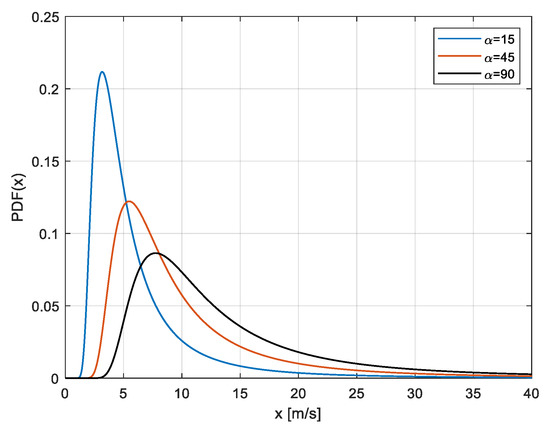
Figure 1.
Various Compound Inverse Rayleigh PDFs, with three different values of the parameter η (the parameter appears in the legend) The values on the x-axis are WS values in m/s.
2.4. Comparison among Similar WS Models
It seems opportune to compare the CIR model with other similar models such as the IR and the Exponential model. Further on, also some hints at a possible approximation with the Pareto CDF—also widely adopted for extreme value data characterization—are illustrated in the present sub-section.
First, the IR and CIR model are examined. Before illustrating the similarity of the two models in their “extreme tails”, it may be shown that such similarity can be motivated analytically by their asymptotic properties, i.e., the fact that the two models become close for large values of the WS. It is simple to note that when the CDF argument diverges, the first-order Mac Laurin series expansions of the IR and CIR CDF tend to become equal. More precisely, by referring to the expressions reported—respectively for the CIR and the IR CDF—in Equations (2) and (5), it is easy to show that, when the WS value x is sufficiently high, the asymptotic expression of the CIR CDF F(x|η) of (2) is:
On the other hand, the asymptotic expression of the IR CDF G(x|α) of (5), here parametrized as is:
So, when x is high enough that , then when and are equal (or not very different).
Then, as hinted at above, it is interesting to compare, in order to get a better knowledge of the two models in their “extreme tails”, the quantiles of the two models, when they possess the same median or 0.50-quantile. So, let m be the common median value. The CIR model is expressible directly in terms of m, of course, being m = η, as follows:
In addition, the IR CDF (as well as the corresponding PDF) is expressible in terms of the median m, as follows, by denoting:
Such re-parameterization can be useful, as remarked in [37,38], in the phase of a proper model identification, since different probability models often imply similar estimated values of “central parameters”—such as the median or mean value—when fitted to the same data, but exhibit different “extreme” tails, i.e., extreme quantiles such as the ones corresponding to values of p equal to p = 0.95 or p = 0.99.
The generic p-quantile of the IR and CIR models—respectively denoted as Xp and X’p, are simply expressible in terms of their median m as follows:
In Table 1, three different p-quantiles (for p = 0.63, 0.95, 0.99, in column 3,4,5) are reported for an IR model (row 2) and a CIR model (row 3) with the same median m = 7 m/s. A not very large value of m has been chosen for sake of illustration, with the purpose to highlight that, also in this case, the extreme quantiles may sometimes be rather different. Moreover, the “large tails” of the above models under studies are also made more evident by reporting the corresponding quantities for a “classical” Exponential model (row 1), i.e., with CDF expressible as follows in terms of the mean value :

Table 1.
Some statistical parameters of the three models for WS with same median = 7 m/s.
For a more complete comparison, the mean (expected) values of the three models are also reported. The one of the Exponential model is reported as a parameter in (23), those of the IR model and the CIR model (as reported above) are respectively:
For the Exponential model, it is well known that m = m, and that the mean is equal to the p-quantile for p = 0.63, which is the reason why this 0.63 quantile is reported, for easier reference with the other models. In all the three cases, the mean is higher than the median, as always happens with unimodal distributions with positive skewness (i.e., with “right tails” [33]).
The curves of the PDF corresponding to the three models are shown in Figure 2.
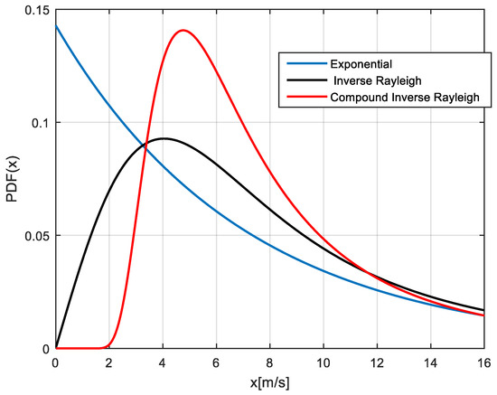
Figure 2.
The curves of the three PDF corresponding to the models (the Exponential, IR, CIR) in Table 1, with the same median value 7 m/s.
It is clearly apparent, from the values reported in Table 1, as also from the curves, that, although possessing the same median (and about the same mean)—or more generally being similar in their central part” (including the 0.63-quantile)—the IR and CIR models behave quite different in their extreme right tails, the one of the CIR model being much larger than the one of the IR model. For instance, the 0.95-quantile has a 18% increase from the IR to the CIR model, while the 0.99-quantile has a 20% increase. Both models, of course, possess larger tails when compared to the Exponential model.
It is remarkable that the above right-hand sides in Equations (16) and (17) can be seen as a particular case of the Pareto distribution (although only for very large x values), a very classical model for describing the extreme values distribution [31,32,33]. The Pareto CDF has the following expression (which, if h = 2, is the same expression as (14) and (15) for finite values of x):
A similar argument also applies to the Inverse Log-logistic and the Inverse Burr models [28,29]. (the latter is also known in the literature as “Dagum distribution” [42]), whose CDF can be expressed respectively as follows:
being β, τ, γ all positive parameters.
3. Application of the CIR Model to Real Wind Speed Datasets
The results reported in the present Section 3 serve as a validation of the proposed CIR model. In order to better emphasize that the validation is satisfactory, this Section is fairly long, with many tables—i.e., Table 2, Table 3 and Table 4—and figures—i.e., Figure 3a–d and Figure 4a–d—which clearly demonstrate the validity of the CIR model to interpret different field data (of course, this does not mean that it can interpret all data). All the results reported here refer to real wind speed data, and the many relevant statistical fitting results reported in Table 3 and Table 4 and in the Figures show, for the sets of reported data, the superiority of the CIR model with respect to other alternative models that are being used in the literature and in real applications.
Table 2.
Size and statistical characteristics of the datasets used in the experiments.
Table 3.
Goodness of fit of the CIR distribution and of the benchmark distributions on the PM EWS datasets. Bold values indicate the best results for each location.
Table 4.
Goodness of fit of the CIR distribution and of the benchmark distributions on the POT EWS datasets. Bold values indicate the best results for each location.
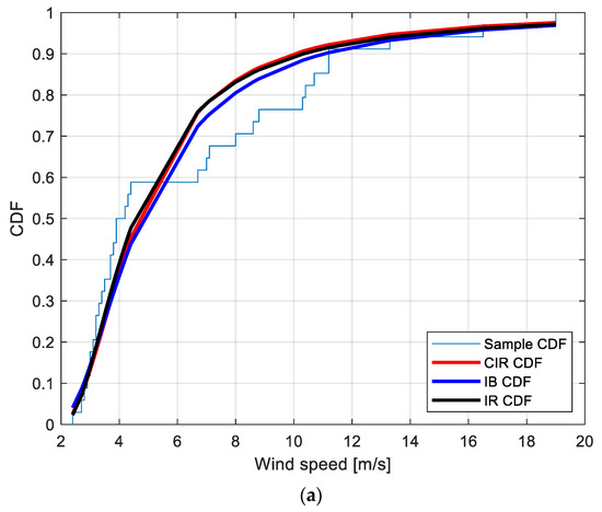
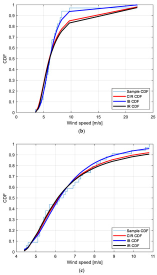
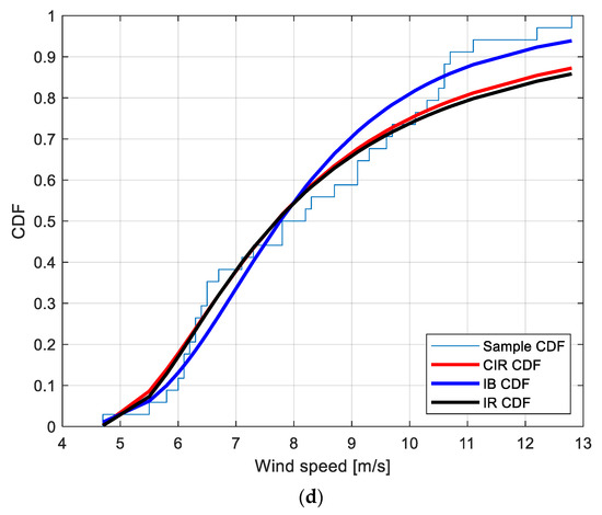
Figure 3.
Sample CDF and fitted CIR, IB and IR distributions for the PM EWS at the locations: (a): Amintayo; (b): Beui; (c): Koilada; (d): Pontokomi.
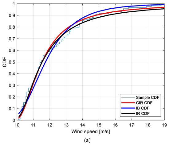
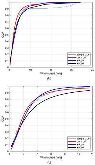
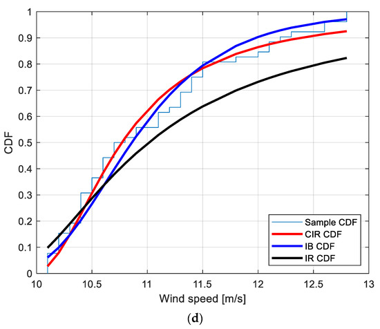
Figure 4.
Sample CDF and fitted CIR, IB and IR distributions for the POT EWS at the locations: (a): Amintayo; (b): Beui; (c): Koilada; (d): Pontokomi.
3.1. EWS Datasets
The CIR model is applied to characterize real-world data collected at several locations in Greece in 2012 [25,26]. Data consist of hourly observations of wind speed, from which the EWS are extracted in terms of Period-Maxima (PM) EWS and Peaks-Over-Threshold (POT) EWS. PM values are the maximum WS values in a given time interval (one week for the present data set), while POT values are only the WS values which are greater than a given threshold value. Four locations that significantly differ in terms of wind speed characteristics are presented in this Section: Amintayo, Beui, Koilada, and Pontokomi.
In order to keep the dimensions of data consistent, the threshold picked for building the POT EWS dataset is not the same across the locations. It is set at 10 m/s for locations Amintayo and Pontokomi, and 5 m/s for Beui and Koilada. With reference to the PM EWS dataset building, the period considered is 1 week for all four locations. With this approach, the eight considered datasets have the size and the statistical characteristics presented in Table 2.
The goodness of fit of the CIR distribution upon these data is compared to the goodness of fit of other benchmark distributions that are typically used for EWS characterization, i.e., the Inverse Burr (IB) distribution, the Inverse Weibull (IW) distribution, the Gumbel (GU) distribution [33], and the Inverse Rayleigh (IR) distribution.
To evaluate the performance of the CIR distribution and to compare it with the benchmark distributions, the outcomes of the Kolmogorov–Smirnov (KS) test [41,42], i.e., the KS test statistics (), is presented. The Adjusted Determination Coefficient (ADC) is presented too, in order to account for the number of parameters in each distribution [41].
3.2. Period-Maxima EWS Characterization
The results for the PM EWS characterization are shown in Table 3. Bold values indicate the best results for each location.
The CIR distribution has overall the best performance for the locations Koilada and Pontokomi, and it also shows the smallest KS test statistic for the location Amintayo (note that the CIR for the Amintayo location is only slightly smaller than the greatest value achieved by the IW distribution). Nevertheless, the CIR distribution is not suitable to characterize the PM EWS at the Beui location, as it is unable to reach performance close to the IB distribution, which is the best pick for this location. In only one case (i.e., the GU distribution for the location Amintayo) the KS test was not successful.
With the purpose of providing a graphical interpretation of the fitting, Figure 3a–d show the sample CDF and the fitted CIR, IB, and IR distributions, for the Amintayo, Beui, Koilada, and Pontokomi locations, respectively.
3.3. Peak-Over-Threshold EWS Characterization
The results for the POT EWS characterization are shown in Table 4. Bold values indicate the best results for each location.
The CIR distribution always returns the smallest KS test statistic and the greatest , in all the considered locations, denoting an overall better fitting than the fitting of PM EWS.
To provide a graphical interpretation of the fitting, Figure 4a–d show the sample CDF and the fitted CIR, IB, and IR distributions, for the Amintayo, Beui, Koilada, and Pontokomi locations, respectively.
4. A Bayes Method of Inference for the CIR Model
4.1. A Premise on the Proposed Method
Since it is analytically straightforward, the classical statistical approach for the estimation of the CIR model is only hinted at in the next section, while in this section the Bayes method of inference is summarized, and then applied to the CIR model. As well known, in the classical statistical approach [41], featuring (among the others) the method of moments and the maximum likelihood (ML) method of estimation, any parameter to be estimated is seen as a fixed but unknown variable. Instead, in Bayesian parameter estimation [39,40,41,43], each unknown parameter is seen as a random variable, so that it possesses a “prior” PDF representing the probabilistic information or the “belief” of the observer about the parameter.
Then, letting the parameter (possibly a vector) denoted by w, its prior PDF g(w) is integrated and updated with field data—denoted by D—by the below reported well known Bayes’ theorem, which allows to obtain the the posterior distribution g(w|D) of w, conditional to the observed data D:
where:
- L(D|w) denotes the Likelihood (i.e., the joint PDF in the present case) of the data D conditional to the parameter w;
- C is a constant (with respect to the parameter values), obtained by the “normalizing” integral:
The above integral is a multiple one, in the case w is a vector of parameters, say: w = (w1, w2, …,wp), so that dw = dw1, dw2, …, dwp.
In a Bayesian analysis, the posterior distribution sums up the current status of knowledge about the unknown parameters of probability distributions, integrating the prior knowledge (before data observation)—or the initial belief about the parameter—represented by the prior distribution, and the knowledge produced by data in terms of the likelihood function of the observed data, which in a sense measures the information contained in the data. Once the posterior distribution, here in terms of posterior PDF g(w|D) of (29), has been deduced, there are various possible choices for the Bayes point estimate of the parameter w. A very common choice, as the “best” Bayes estimate—in the mean square error sense—is the posterior mean of such PDF. As is well known [39], such an estimate minimizes the posterior mean squared error.
Another popular choice, here performed, is the so called “Maximum a Posteriori Probability” (MAP) estimation, in which the point estimate w° of the parameter w is the value which maximizes the posterior PDF g(w|D):
where Sw is the parameter space, i.e., the set of all possible values that w can assume. This choice, which by definition maximizes the probability of a correct estimation (or minimizes the estimation error probability), constitutes a “classical” method in Bayesian analysis and has gained new interest in the last years, also being adopted in the framework of the recent machine learning methods [44,45,46].
Both the posterior mean and the MAP estimator, as will be apparent from the following equations, require numerical methods, but the MAP estimator is somewhat simpler to compute, being nonetheless very close to the posterior mean.
In view of the estimation of the CIR model, the parameter w to be estimated, appearing in Equations (29)–(31), i.e., the “input” of the estimation process, may naturally be the parameter η of (2)–(4), also reported in the following Equation (32). The parameter η also represents the median of the CIR distribution. However, also any other parameter τ = τ(η) related to the unknown parameter η may be chosen as the input parameter. It is recalled that, in the Bayesian methodology, also any functions of the random parameter η are themselves RV, described by appropriate distributions. In particular here, once a given WS value x has been fixed, the attention may be focused on the inference on value of the CIR CDF at x:
Indeed, also the CDF—as well as other parameters (e.g., moments and quantiles)—may be considered as the input of the estimation process. It is remarked that, although formally equal to Equation (2), the expression in (32) should not be seen as a function of the WS x, which is instead a fixed constant there. This is indeed a function of the unknown parameter η, thus constituting a new parameter, on which it should be easy to assess a prior PDF. For mathematical convenience, alternatively, by introducing the new RV:
the above expression of the CIR CDF can be re-parametrized (omitting for clarity the dependence on x, which is a constant, so writing F instead of F(x)):
Of course, assessing a prior PDF on the random parameter η implies—being x a given constant—assessing a prior PDF on the random parameter Y, as well as on F and other related parameters. Of course, the converse is also true. The choice of the most convenient way depends on the kind of information that the observer possesses.
For instance, a reasonable prior assessment could be the one assessing the probability that the WS is higher than a given value x: this seems indeed a realistic piece of information, which should be available to the engineer based on past WS data. By the above relation, such “exceedance probability” is expressed by:
being S(x) = 1 − F(x) the “Survival function” of the WS RV. It is interesting to remark that this can be considered as a “un-safety index”, accounting for the most severe EWS amplitudes as disturbances for wind tower safety.
In summary, for the above estimation, two methods are considered in the paper in order to establish an appropriate prior distribution as illustrated in the following sub-sections, i.e., assessing assigning a Lognormal prior distribution to the parameter η (Section 4.1.), or a Beta prior distribution to the parameter S (Section 4.2). Although, in general, the two prior assessments (i.e., assessing a prior distribution to the parameter η or a prior distribution to the parameter S) can be made equivalent by appropriate choice of the relevant prior PDF parameters, choosing one or the other as the basic input information has some peculiar analytical aspects that are highlighted in the following, since—for instance—a Lognormal prior distribution on the parameter η does not imply a Beta prior distribution on the parameter S, but a so-called “Beta-Lognormal” distribution discussed in the following. However, such “Beta-Lognormal” distribution can be nonetheless approximated to a certain extent by a Beta distribution.
Finally, it is remarked that the choice of assessing a prior distribution to the parameter S is in accordance with the so-called “practical” Bayes estimation, which is widely adopted nowadays in various applications, after being first proposed in [36] in the framework of reliability analyses.
4.2. “First Approach”: Choice of a Lognormal Prior Distribution of the Parameter η
Let us examine the first choice, for which a Lognormal prior PDF is suggested for its great flexibility and for its easy transformation into the corresponding prior PDF for the above introduced RV Y and S, when needed. Let η be a Lognormal RV, with the following PDF [33]:
The function g(η) is zero for η < 0; parameters γ, β are respectively the scale and the shape parameters of the Lognormal PDF. Then, by virtue of (33), also Y is an opportune Lognormal RV, because of known properties of the Lognormal model [33] (among which, the fact that—given a Lognormal RV Y—any power function, Yk is still a Lognormal RV, whatever the value of the real constant k). The parameters of the PDF of Y are simply deducible from those of η. Then, the RV S of (35) possesses a known PDF, which can be expressed as follows. First, the new RV:
is introduced. It is again a Lognormal RV with PDF, here denoted by h(t), simply expressible in terms of the Lognormal PDF of (36):
T = 1/Y
Then, the PDF of S is easily expressible in terms of the one of T, since:
Then, denoting by q(s) the PDF of S, it can be expressed in terms of the above PDF h(t) of T by means of a “Beta-Lognormal” PDF (introduced in [47]), which—by well-known rules of PDF transformations, is given by:
Of course, since F = 1 − S, the prior PDF of F is also simply expressible. The above PDF should be conveniently approximated by a Beta PDF, as discussed in [47]. Indeed, it is known that a Beta RV, say Z, may be characterized, under some hypotheses, as the ratio Z = U/(U + V) = 1/(1 + W), being U and V independent Gamma RV [33,43], and so W = V/U the ratio of two independent Gamma RV. Because of the known similarity between the Gamma and the Lognormal PDF (for given common values of mean and standard deviation, [46]), it may be expected that also the PDF of Y in (39) may be at least approximated by a Beta PDF, as in our application was successfully verified. Indeed, in the following Section 5 it is shown that the estimation results are not so different when assuming a Lognormal PDF on η (as discussed here), or when assuming a Beta PDF on S, as discussed in the following sub-section.
4.3. “Second Approach”: Choice of a Beta Prior Distribution the Parameter S
With the purpose of assessing the prior information on S, a Beta PDF [33,39,41,43] may be successfully adopted, as generally done for RV in (0,1) [39], due to its great flexibility in this interval. The Beta PDF for S, f(s), with positive parameters (p,q), can be expressed as follows:
It is noticeable that in such case also F = 1 − S is a Beta RV [33], whose PDF can be obtained from (41) simply swapping the roles of parameters (p,q). This choice also implies that the RV Y of (35), which is obtained as a function of S (as simply deducible from (35) itself) by:
is a RV with support (0,), which possesses a so-called “Beta Prime” distribution [33], with the same positive parameters (p,q) of the Beta PDF of S. This means that the PDF u(s) of Y can be expressed as follows:
Such PDF of Y implies in turn an analytical expression also for the parameter η, which is also an RV with support (0,), and by means of (33) is proportional to the square root of Y:
This means that the PDF of η can be still expressed, with some adequate transformation, in terms of the Beta Prime distribution of (43). I.e., given the PDF u(y;p.q) of (43), the implied prior PDF of η, say v(h), is expressed by:
The applications of the above Equations (36) and (45), expressing respectively the prior PDF of η according the first approach and the second approach, have been performed in the course of the computations of the following section, as described afterwards.
Then, both in the case of the first and the second approach, in order to obtain the Bayes estimate (be it the posterior mean or the MAP estimate), the posterior PDF shall be computed according (29), i.e., by multiplying the above prior PDF ((36) or (45), according to the case under study) and the Likelihood function L(D|w). This Likelihood function, which can be denoted by L(D|η), since in this case is the only parameter to be estimated, is the joint PDF of the CIR RV which constitutes the sample of n WS values (x1, x2, …, xn), i.e., it is the product of n PDF f(xj|η) j = 1 …n, such as the one in (3), evaluated in xj (j = 1 …n), being n the sample size.
As far as the MAP estimate is concerned, it is not important to evaluate the constant C in (29), since its value does not change the maximum of the above product g(η) L(D|η). However, the MAP estimate must be obtained numerically (and the same would be true also for the posterior mean or other possible estimates).
5. Numerical Application for Estimation Efficiency Assessment of the Proposed Approach
5.1. Illustration of the Bayes Estimation Results
The present section illustrates a series of numerical applications for assessing the estimation efficiency of the proposed Bayes approach based on a large set of simulated experiments. All the relevant results are expressed in terms of the estimation of the only model parameter, η, here considered as an unknown. Nonetheless, as it was illustrated in previous Section 4.3, in some cases, according to the “second approach”, the primary source of (prior) information will not be considered the information on the parameter, but the information on a given values of the S. This efficiency assessment is carried out in “absolute” terms, as well as in terms of ‘relative efficiency’ [41,42,43,44,45,46] of the Bayes approach compared to the “classical” approach. As is well known [41,43,44,45,46], the classical approach is generally based on the aforementioned ML estimation method, which in the present case can be easily derived from the more general one regarding the EWS model presented in [29]. However, as discussed in [29], such MLE procedure yields sometimes some convergence problems. In such cases, simpler ways to attain parameter estimates are the Method of moments estimation [41] (briefly, “moments estimation”) and the “quantile estimation” (QE) [29] methods. In the case of the CIR model, the moment estimation procedure consists of solving a simple system of one equation, obtained equating the first sample moment (or the “sample mean”, i.e., the average value of WS in the sample) to the theoretical mean value. The QE procedure consists of equating a given sample quantile to the analogous theoretical quantile. Since the parameter η is equal to the median of the CIR model, it is convenient in this case to adopt a QE method by choosing the sample median. As intuitive from previous equations expressing the statistical parameters of the CIR model (showing that the mean and the median are related by a linear relationship), it may be expected that the moment estimation and the QE yield very close estimates for η, as was verified in the course of the computations of the present section. Moreover, in all the applications here presented they resulted practically equal to the MLE. So, for brevity and computational simplicity in the following, the value of the QE estimate is reported as the “classical” estimate.
As hinted at before, the Bayes MAP estimates have been obtained, in each simulation, numerically (since an analytical solution of the above equations is not available), on the basis of the performed simulations which are described in the following sub-sections, respectively for the first and the second approach (i.e., the choice of a Lognormal prior distribution on the parameter h, or the choice of a beta prior distribution on the parameter S, as explained in Section 4).
The results are reported with the following subdivision:
- (1)
- Case A (in Section 5.2), based upon the adoption of a Lognormal prior PDF on parameter η, (i.e., the median),
- (2)
- Case B (in Section 5.3), based upon the adoption of a Beta prior PDF on parameter S.
- (3)
- Case C (in Section 5.4), in which a “robustness analysis” is illustrated,
The three cases (A,B,C) are further subdivided into more sub-cases (A1–A3, B1–B3, C1–C4), as explained in the following.
5.2. Case A: Bayes Estimation Results for the “First Approach” (Choice of a Lognormal prior Distribution on the Parameter η)
Table 5, Table 6 and Table 7 illustrate the results of 3 sets of simulation cases, among the many more performed, in which a Lognormal prior PDF g(η; β,γ) as in (36) is assumed for η, with prior mean E[η] = 11.5 m/s, and three different values of prior coefficient of variation (CV), namely the ratio between standard deviation and mean value), i.e., the following CV values:
CV[η] = 0.150 (case A1); CV[η] = 0.150 (case A2); CV[η] = 0.050 (case A3)
Table 5.
Estimation efficiency: numerical results for case A1.
Table 6.
Estimation efficiency: numerical results for case A2.
Table 7.
Estimation efficiency: numerical results for case A3.
These three different assumptions yield indeed the three sub-cases A1, A2, A3, reported below together with the corresponding values of the above introduced Lognormal prior PDF (β,γ) of (36), namely:
- Case A1: CV[η] = 0.150 (γ = 2.4312; β = 0.1492);
- Case A2: CV[η] = 0.100 (γ = 2.4374; β = 0.0998);
- Case A3: CV[η] = 0.050 (γ = 2.4411; β = 0.0500).
These three cases are selected to highlight different degrees of prior uncertainty; indeed, a greater prior CV involves a greater degree of prior uncertainty, thus the estimates are expected to be less efficient when examining the results from case A1 to case A3, as will be confirmed to some extent by the results hereafter. Out of the above cases, case A1 is to be considered the “worst” case since it possesses the highest CV value. In Figure 5, the Lognormal prior PDF of case A2 for η is shown.
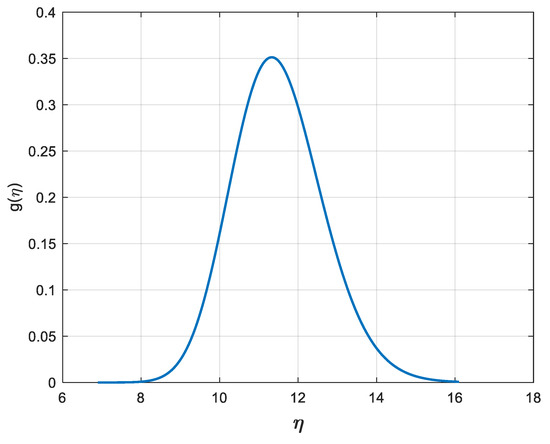
Figure 5.
Lognormal prior PDF of η in case A2, with mean 11.5 m/s and CV = 0.10 (as in Equation (36), with parameter values: γ = 2.4374; β = 0.0998).
For all the considered cases, Monte Carlo simulations (each one performed with n = 104 simulated samples of various sizes) have been used as a tool to evaluate the efficiency of the Bayes estimates, relying on the well-known basic statistics listed here below [39,41,43], all referred to the estimation of η:
- Mean Square Error of the Bayes estimator (BMSE);
- Mean Square Error of the classic estimator (CMSE);
- Relative Efficiency of the Bayes estimator with respect to the Classic estimator (REFF = CMSE/BMSE).
It is recalled that the classic estimator may be here computed as the MLE or the QE estimator, since the two values are in practice always very close; the figures in the tables are referred to the latter, which has the advantage of easier and faster computation. The most popular quantitative way to assess the ‘relative efficiency’ of the Bayes estimator compared to the classic estimator is the REFF index: the more REFF overcomes unity, the more efficient is the Bayes estimate compared to the classic estimate. Furthermore, the meaningful “accuracy indexes” listed here below were also considered as a quantitative way to assess the “relative bias” (or the “precision”) of the Bayes estimator [39], which should of course be as small as possible:
- Mean Relative Error of the Bayes estimator (BMRE);
- Maximum Relative Error of the Bayes estimator (BMAXRE).
In all simulated samples for the estimation of η, the estimates are carried out for different values of sample size n—as usually happens in reality—which can be classified as small, i.e., n = 5, 10, and moderately large, i.e., n = 20, 30.
It is apparent from the above tables that, as desired, the indexes BMSE, BMRE and BMAXRE are very limited, while the REFF index is always larger, often much larger than 1 (unless the sample size and/or the prior CV are relatively high), accounting for a very efficient estimation procedure. A more detailed discussion of the reported results is postponed to the end of the next sub-section, in order to examine also the cases (B1, B2, B3) relevant to the “second approach”.
5.3. Case B: Bayes Estimation Results for the “Second Approach” (Choice of a Beta Prior Distribution the Parameter S)
According to the same methodology as in the previous sub-section, here we illustrate the results of 3 sets of simulation cases, among the many more performed, in which the previously discussed choice of a Beta PDF on the Survival function S = S(x), at x = 11.5 m/s is adopted. All the cases reported here are relevant to a prior mean E[S] = 0.5 at x = 11.5 m/s (which is—in a probabilistic sense—to a certain degree equivalent to assuming a prior mean of the median having value of 11.5 m/s, as in cases A). As in case A, the same three different assumptions on the prior CV are held, originating the three sub-cases B1, B2, B3, reported below together with the corresponding values (p,q) of the beta prior PDF u(p,q) of (43):
- Case B1: CV[S] = 0.150 (p = q = 21.722);
- CaseB2: CV[S] = 0.050 (p = q = 49.500);
- CaseB3: CV[S] = 0.025 (p = q = 199.500).
In Figure 6. the Beta prior PDF of case B1 for S is shown.
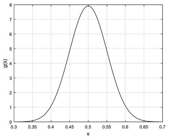
Figure 6.
Beta prior PDF of S of case B1, with mean 0.5 and CV = 0.15 (as in Equation (43), with parameter values: p = q = 21.722).
Again, the same indices (BMSE, etc.) are reported as in cases A1–A3. Such indices are all still referred to the estimation of η, for an easier comparison with previous results. For the sake of brevity, since the results for cases B2 and B3 (available on request from the authors) are similar (and often better, i.e., with higher REFF values) to those of cases A2 and A3, only the numerical results for case B1 (the “worst” case among the cases B1–B3) are reported in Table 8. Given the same prior CV values (0.150), the numerical results for case B1 in Table 8 may be compared to those for case A1 in Table 5.
Table 8.
Estimation efficiency: numerical results for case B1.
5.4. Case C: Bayes Estimation Results Relevant to a Robustness Analysis
The numerical assessment of Bayes approach efficiency is closed by a “robustness” analysis [39] with respect to the choice of the prior distribution (but always retaining, except in the last case, the same values of the assumed prior mean and CV). The purpose of a robustness analysis is to certify, to a certain degree, that the performance of the estimation method is not so much sensitive with respect to “wrong” prior assumptions, in a sense which will be better clarified afterwards.
In the cases examined here, and illustrated by the last four Table 9, Table 10, Table 11 and Table 12, it is hypothesized that the Bayes computations are performed assuming a “wrong” prior distribution, be it the Lognormal model of case A for η or the Beta model of case B for S. Instead, a different prior distribution generates the true values of η or S. In detail, the following more cases are illustrated in Table 9, Table 10, Table 11 and Table 12, indicated overall as “Case C”, with the following subdivision:
Table 9.
Robustness: numerical results for case C1.
Table 10.
Robustness: numerical results for case C2.
Table 11.
Robustness: numerical results for case C3.
Table 12.
Robustness: numerical results for case C4.
- Case C1: The prior distribution of η is Normal, with the same mean (11.5 m/s) and CV = 0.15 of the assumed prior distribution of η, which is the Lognormal prior PDF of case A1;
- Case C2: The prior distribution of η is Uniform, with the same mean (11.5 m/s) and CV = 0.15 of the assumed prior distribution of η, which is again the Lognormal prior PDF of case A1. This implies that the prior distribution of η is Uniform in the interval (a,b), with: a = 8.5122; b = 14.4878;
- Case C3: The prior distribution of S is Uniform, with the same mean (0.50) and CV = 0.15 of the assumed prior distribution of S, which is the Beta prior PDF of case B1. This implies that the prior distribution of S is Uniform in the interval (a,b), with: a = 0.3701; b = 0.6299;
- Case C4: The prior distribution of S is Uniform in (0,1), while the assumed prior distribution of S which is the Beta prior PDF of case B1. This implies that the prior distribution of S has the same mean (0.50) of the assumed prior, but a quite different CV (0.5477).
The four cases are representative of a wide range of cases in which the assumed prior PDF is a wrong one, and in particular, in the last case C4, a very wrong assumption is hypothesized, since the Uniform PDF in (0,1) is very different from the Beta PDF; the Uniform PDF possesses a mean value 0.5 and, as well known [33], a standard deviation equal to 1/√12, and thus a CV equal to 2/√12 ≈ 0.5477.
It is remarked that, in any case, the less favourable prior PDFs are adopted as the reference models, i.e., those of cases A1 and B1, possessing the highest values of the CV.
6. A Discussion on the Results, the Proposed Model, its Limitations and Further Expansions
The present section discusses the results reported in the previous section, as well as its limitations and suggestions for future possible expansions of the model.
As a general comment to the results reported in the previous section, in Table 5, Table 6, Table 7 and Table 8, first a look should be given to each single table, examining the results referred to the various sample sizes. In any of the three cases referred to in Table 5, Table 6 and Table 7 for case A, and in Table 8 for case B, the results about the efficiency of the proposed Bayesian approach are very satisfactory. Indeed, the Bayes estimate errors (in terms of BMSE) are reasonably limited, for each value of n. Moreover, the relative efficiency (REFF index) with respect to the classic estimate is always larger than 1, not only for small sample sizes (n = 1, 3), as expected, but also for sample sizes as large as n = 30 (of course, as well known [39], the REFF index generally decreases with n).
Looking in sequence at the three Table 5, Table 6 and Table 7 for cases A1 to A3, respectively, the efficiency of the Bayes estimates is seen to increase from case A1 to A3 (and the same occurs also from case B1 to B3—cases B2 and B3 are omitted here for the sake of brevity). This was to be expected, since the prior precision (as measured by the prior CV) increases as the CV decreases, as occurs from case A1 to A3. Nonetheless, the results show that also in cases A1 and B1—the “worst” cases reported here (i.e., those implying the highest CV value)—an excellent efficiency is exhibited. This is true both in absolute terms and with respect to the classic estimation results. Moreover, the estimation efficiency seems mostly greater for cases B than for cases A, as confirmed by the above hinted comparison between case A1 (in Table 5) and case B1 (in Table 8).
Similar considerations to those regarding the estimation efficiency can be made with respect to the precision of the estimates, described by the indices BMRE and BMAXRE, which are always very small; this feature appears to a certain extent independent of the sample size.
Considering, then, the robustness analysis of Section 5.4, the reported results show that the efficiency and the precision of the estimates is not so sensitive to “wrong” assumptions on the prior distribution, at least when the values of the assumed prior mean and CV are the “correct” ones. Indeed, the REFF index is less than 1 in only three cases: one is relevant to the case C2 with sample size n = 30, the other two are relevant to the case C4 with sample size n = 20 and n = 30; this may be not surprising, given—in such cases—the large difference between the assumed prior model and the true prior model, and the high value of CV and sample size. In such cases, nonetheless, the very low values of the BMSE should be noticed.
It is remarked that the above terms “wrong” and “correct” are to be interpreted with a certain degree of caution, since—in the framework of the Bayes inference—the prior assumptions have the meaning of personal or subjective beliefs, based upon the experimenter’s experience or past data, and should not be justified. Nonetheless, in order that the results could be, in a sense, also accepted in the framework of an objective estimation philosophy [39], the robustness appears to be a very desirable property, also aimed at circumventing possible criticisms that “ad hoc” prior assumptions are made with the purpose of obtaining the desired results.
Finally, the proposed Bayes estimation method appears to be both efficient and robust. It is remarked that the proposed method of estimation appears to be simple and very practical at the same time, since it only requires some prior guess on the median of the EWS distribution, or on the probability that the wind speed is larger than a given value, and that this choice could be expressed by very simple and flexible prior distributions, such as the Beta and the Lognormal models.
In summary, while the above derivation (Section 2), validation and applications to real data (Section 3) constitute, in the authors’ opinion, the basis for judging the proposed model as a satisfactory model for EWS applications, it seems also opportune to briefly discuss its limitations.
First of all, the CIR model—being characterized by a single-parameter PDF—is not expected to be flexible enough to describe more complex PDFs as those sometimes adopted to model extreme wind speed data, such as the “generalized extreme value distribution” [18].
From a more general point of view, the CIR model—as also happens with popular and typically adopted models, e.g., the Weibull—is not adequate to model wind speed data which exhibit a certain degree of correlation among them: for such data, time series or other more complex methods, such as neural networks, appear worth being investigated: recent developments in the time series approach are illustrated in [48,49], while those in neural networks applications are illustrated in [49,50,51,52].
Dealing with correlation, in the framework of marine structures safety, it is apparent that a correlation between random wind and wave processes can be established for the random vibration analysis of marine structures. In particular, coherence and cross-spectral density matrix analysis of random wind and wave in deep water are the object of recent studies such as [53].
7. Conclusions
In the paper, the Compound Inverse Rayleigh model has been motivated for the probabilistic characterization of extreme values of wind-speed, also illustrating its validity in interpreting real wind-speed data sets. Before introducing its practical adoption to real data sets, and then its estimation, the model has been deduced analytically as a mixture of Inverse Rayleigh models (a mixture which originates the model’s denomination), also discussing with some detail its comparison with other more popular distributions adopted for extreme wind-speeds, such as the Pareto, Gumbel, Inverse Weibull, Inverse Burr and more.
Later on, the statistical estimation of the model has been developed by means of a novel Bayes estimation method, whose feasibility, efficiency and precision have been illustrated by numerical examples and a broad amount of Monte Carlo simulations performed relying on typical values of real extreme wind speed data. Different performance indexes, such as the MSE, the “Relative Efficiency”, the “Mean Relative Error” and the “Maximum Relative Error” indices, have been evaluated with the purpose of a thorough assessment of the performance of the estimation method, with very satisfactory results. In the final section, a numerical analysis is devoted to the robustness assessment of the methodology (i.e., using prior distributions different from the ones chosen here), again with good results., showing that the estimation efficiency holds, at least in most of the examined cases, also when the true prior model is rather different from the one assumed for the computations. This Bayesian approach constitutes a “practical” statistical method for the estimation of the above distribution parameter from available data, proposing two alternative, simple prior models, the Beta and the Lognormal models, for the prior information assessment of a model quantile or of the model Survival Function. Such results prove the good performance of the proposed approach, especially with respect to classical estimation methods.
It is deemed that the proposed model is a valid tool to accomplish both the necessity of an efficient assessment of wind tower safety, and the necessity of a valid characterization of the statistical parameters of wind-power generation, which is also dependent on the above extreme values, e.g., in view of the establishment of the cut-off threshold. The two aspects are in fact related to each other since the crossing by part of the WS of the speed cut-off threshold annihilates the generated power, and at the same time may pose a severe threat to the mechanical safety of the wind structures.
In synthesis, it is remarked that:
- (1)
- from the probabilistic point of view, the proposed CIR model is a new EWS model which can be useful for many applications relevant to the analysis of real EWS data. This is shown from its derivation by means of a mixture (Section 2), and most importantly from its validation, i.e., the verification of its capability of interpreting numerous real EWS data (Section 3)
- (2)
- from the statistical point of view, the novel practical Bayes estimation procedure that has been proposed for the CIR model is a very efficient and robust one.
Author Contributions
Conceptualization, E.C.; methodology E.C.; validation, E.C. and G.M.; formal analysis, E.C. and M.F.; investigation, E.C., M.F. and G.M.; writing—original draft preparation, E.C.; writing—review and editing, E.C., M.F. and G.M. All authors have read and agreed to the published version of the manuscript.
Funding
This research received no external funding.
Acknowledgments
The authors are grateful to Pasquale De Falco for helping the authors in finding the datasets for the application of Section 3 and performing the computations of the relevant statistics.
Conflicts of Interest
The authors declare no conflict of interest.
Nomenclature
| ADC | Adjusted Determination Coefficient |
| CIR | Compound Inverse Rayleigh distribution |
| CV | Coefficient of variation |
| CV[Z] | Coefficient of variation of a RV Z |
| CDF | Cumulative distribution function, F(x) |
| EWS | Extreme wind speed |
| E[Y] | Mean (expected) value of the RV Y |
| GU | Gumbel Distribution |
| IB | Inverse Burr distribution |
| IR | Inverse Rayleigh distribution |
| IW | Inverse Weibull distribution |
| KS | Kolmogorov–Smirnov test |
| Probability density function, f(x) | |
| PM | Period Maxima |
| POT | Peaks-Over-Threshold |
| m | generic median |
| η | median of the Compound Inverse Rayleigh distribution |
| WS | Wind speed |
| QE | Quantile estimation |
| ML, MLE | Maximum Likelihood, Maximum Likelihood estimate |
| RV | Random variable |
| S, S(x) | Survival function, S(x) = 1 − F(x) |
| m | mean value (expectation) of a RV |
| s2, s | Generic variance and standard deviation of a RV |
| z° | denotes a Bayes estimate of the parameter z |
References
- Jain, P. Wind Energy Engineering; McGraw-Hill: New York, NY, USA, 2011. [Google Scholar]
- Manwell, J.F.; McGowan, J.G.; Rogers, A.L. Wind Energy Explained: Theory, Design and Application; John Wiley & Sons: Chichester, UK, 2010. [Google Scholar]
- Letcher, T. Wind Energy Engineering: A Handbook for Onshore and Offshore Wind Turbines, 1st ed.; Academic Press; Elsevier: Amsterdam, The Netherlands, 2017. [Google Scholar]
- Pryor, S.C.; Barthelmie, R.J.; Bukovsky, M.S.; Leung, L.R.; Sakaguchi, K. Climate change impacts on wind power generation. Nat. Rev. Earth Environ. 2020, 1, 627–643. [Google Scholar] [CrossRef]
- Dhiman, H.S.; Deb, D. Probability distribution functions for short-term wind power forecasting. In Proceedings of the 8th International Workshop on Soft Computing Applications (SOFA 2018), Arad, Romania, 13–15 September 2018; pp. 60–69. [Google Scholar]
- Scarabaggio, P.; Grammatico, S.; Carli, R.; Dotoli, M. Distributed demand side management with stochastic wind power forecasting. IEEE Trans. Control Syst. Technol. 2022, 30, 97–112. [Google Scholar] [CrossRef]
- Maldonado-Correa, J.; Solano, J.C.; Rojas-Moncayo, M. Wind power forecasting: A systematic literature review. Wind. Eng. 2021, 45, 413–426. [Google Scholar] [CrossRef]
- Carta, J.A.; Ramırez, P.; Velazquez, S. A review of wind speed probability distributions used in wind energy analysis. Case studies in the Canary Islands. Renew. Sustain. Energy Rev. 2009, 13, 933–955. [Google Scholar] [CrossRef]
- Jung, C.; Schindler, D. Global comparison of the goodness-of-fit of wind speed distributions. Energy Convers. Manag. 2017, 133, 216–234. [Google Scholar] [CrossRef]
- Jung, C.; Schindler, D. Wind speed distribution selection—A review of recent development and progress. Renew. Sustain. Energy Rev. 2019, 114, 109290. [Google Scholar] [CrossRef]
- Ahsan ul Haq, M.; Srinivasa Rao, G.; Albassam, M.; Aslam, M. Marshall–Olkin Power Lomax distribution for modeling of wind speed data. Energy Rep. 2020, 6, 1118–1123. [Google Scholar] [CrossRef]
- Zhang, Y.; Wang, J.; Wang, X. Review on probabilistic forecasting of wind power generation. Renew. Sustain. Energy Rev. 2014, 32, 255–270. [Google Scholar] [CrossRef]
- Zhang, Y.; Pan, G.; Zhao, Y.; Li, Q.; Wang, F. Short-term wind speed interval prediction based on artificial intelligence methods and error probability distribution. Energy Convers. Manag. 2020, 224, 113346. [Google Scholar] [CrossRef]
- Tizgui, I.; el Guezar, F.; Bouzahir, H.; Benaid, B. Wind speed distribution modeling for wind power estimation: Case of Agadir in Morocco. Wind. Eng. 2019, 43, 190–200. [Google Scholar] [CrossRef]
- Patel, P.; Shandilya, A.; Deb, D. Optimized hybrid wind power generation with forecasting algorithms and battery life considerations. In Proceedings of the 2017 IEEE Power and Energy Conference at Illinois (PECI), Urbana, IL, USA, 23–24 February 2017; pp. 1–6. [Google Scholar]
- Tavner, P.; Edwards, C.; Brinkman, A.; Spinato, F. Influence of wind speed on wind turbine reliability. Wind. Eng. 2006, 30, 55–72. [Google Scholar] [CrossRef]
- Wang, J.; Qin, S.; Jin, S.; Wu, J. Estimation methods review and analysis of offshore extreme wind speeds and wind energy resources. Renew. Sustain. Energy Rev. 2015, 42, 26–42. [Google Scholar] [CrossRef]
- Soukissian, T.H.; Tsalis, C. The effect of the generalized extreme value distribution parameter estimation methods in extreme wind speed prediction. Nat. Hazards: J. Int. Soc. Prev. Mitig. Nat. Hazards 2015, 78, 1777–1809. [Google Scholar] [CrossRef]
- Yan, Z.; Liang, B.; Wu, G.; Wang, S.; Li, P. Ultra-long return level estimation of extreme wind speed based on the deductive method. Ocean. Eng. 2020, 197, 106900. [Google Scholar] [CrossRef]
- Chiodo, E.; di Noia, L.P. Stochastic extreme wind speed modeling and Bayes estimation under the inverse Rayleigh distributions. Appl. Sci. 2020, 10, 564. [Google Scholar] [CrossRef]
- Diriba, T.A.; Debusho, L.K. Modelling dependency effect to extreme value distributions with application to extreme wind speed at Port Elizabeth, South Africa: A frequentist and Bayesian approaches. Comput. Stat. 2020, 35, 1449–1479. [Google Scholar] [CrossRef]
- Akgül, F.G.; Şenoğlu, B.; Arslan, T. An alternative distribution to Weibull for modeling the wind speed data: Inverse Weibull distribution. Energy Convers. Manag. 2016, 114, 234–240. [Google Scholar] [CrossRef]
- Chiodo, E.; Mazzanti, G.; Karimian, M. Bayes estimation of Inverse Weibull distribution for extreme wind speed prediction. In Proceedings of the 2015 International Conference on Clean Electrical Power (ICCEP), Taormina, Italy, 16–18 June 2015; pp. 639–646. [Google Scholar]
- Gross, J.; Heckert, N.; Lechner, J.; Simiu, E. A study of optimal extreme wind estimation procedures. In Proceedings of the 9th International Conference on Wind Engineering, New Delhi, India, 9–13 January 1995; pp. 69–80. [Google Scholar]
- Efthimiou, G.C.; Hertwig, D.; Andronopoulos, S.; Bartzis, J.G.; Coceal, O. A statistical model for the prediction of wind-speed probabilities in the atmospheric surface layer. Bound. Layer Meteorol. 2017, 163, 179–201. [Google Scholar] [CrossRef]
- Efthimiou, G.C.; Kumar, P.; Andronopoulos, S.; Giannissi, S.G. Prediction of the wind speed probabilities in the atmospheric surface layer. Renew. Energy 2017, 132, 921–930. [Google Scholar] [CrossRef]
- An, Y.; Pandey, M.D. A comparison of methods of extreme wind speed estimation. J. Wind. Eng. Ind. Aerodyn. 2005, 93, 535–545. [Google Scholar] [CrossRef]
- Chiodo, E.; de Falco, P. The inverse Burr distribution for extreme wind speed prediction: Genesis, identification and estimation. Electr. Power Syst. Res. 2016, 141, 549–561. [Google Scholar] [CrossRef]
- Chiodo, E.; de Falco, P.; di Noia, L.P.; Mottola, F. Inverse Log-logistic distribution for extreme wind speed modeling: Genesis, identification and Bayes estimation. AIMS Energy 2018, 6, 926–948. [Google Scholar] [CrossRef]
- Gross, J.; Heckert, A.; Lechner, J.; Simiu, E. Novel extreme value estimation procedures: Application to extreme wind data. In Extreme Value Theory and Applications; Galambos, J., Lechner, J., Simiu, E., Eds.; Kluwer Academic Publishers: Dordrecht, The Netherlands, 1994; pp. 139–158. [Google Scholar]
- Heckert, N.; Simiu, E. Extreme wind distribution tails: A peaks over threshold approach. J. Struct. Eng. 1996, 122, 539–547. [Google Scholar]
- Heckert, N.; Simiu, E.; Whalen, T. Estimates of hurricane wind speeds by peak over threshold method. J. Struct. Eng. 1998, 124, 445–449. [Google Scholar] [CrossRef]
- Johnson, N.L.; Kotz, S.; Balakrishnan, N. Continuous Univariate Distributions, 2nd ed.; Wiley: New York, NY, USA, 1995; Volumes 1 and 2. [Google Scholar]
- Soliman, A.; Amin, E.A.; Abd-El Aziz, A.A. Estimation and prediction from Inverse Rayleigh distribution based on lower record values. Appl. Math. Sci. 2010, 4, 3057–3066. [Google Scholar]
- Feroze, N.; Aslam, M. On posterior analysis of inverse Rayleigh distribution under singly and doubly type II censored data. Int. J. Probab. Stat. 2012, 1, 145–152. [Google Scholar] [CrossRef][Green Version]
- Erto, P. The inverse Weibull survival distribution and its proper application. arXiv 2013, arXiv:1305.6909. [Google Scholar]
- Chiodo, E.; Mazzanti, G. Theoretical and practical aids for the proper selection of reliability models for power system components. Int. J. Reliab. Saf. 2008, 2, 99–128. [Google Scholar] [CrossRef]
- Chiodo, E.; Mazzanti, G. Mathematical and physical properties of reliability models in view of their application to modern power system components. In Innovations in Power Systems Reliability; Anders, G.J., Vaccaro, A., Eds.; Springer: Berlin/Heidelberg, Germany, 2011; pp. 59–140. [Google Scholar]
- Press, S.J. Subjective and Objective Bayesian Statistics: Principles, Models, and Applications, 2nd ed.; Wiley: New York, NY, USA, 2002. [Google Scholar]
- Erto, P. New practical Bayes estimators for the 2-parameters Weibull distribution. IEEE Trans. Reliab. 1986, 31, 194–197. [Google Scholar] [CrossRef]
- Casella, G.; Berger, R.L. Statistical Inference, 2nd ed.; Duxbury Press: Pacific Grove, CA, USA, 2001. [Google Scholar]
- Kleiber, C. A Guide to the Dagum Distributions; Springer: New York, NY, USA, 2008. [Google Scholar]
- Papoulis, A.; Pillai, S.U. Probability, Random Variables, and Stochastic Processes; McGraw-Hill: New York, NY, USA, 2002. [Google Scholar]
- DasGupta, A. Probability for Statistics and Machine Learning: Fundamentals and Advanced Topics; Springer Science & Business Media: Berlin/Heidelberg, Germany, 2011; Available online: https://link.springer.com/book/10.1007/978-1-4419-9634-3 (accessed on 30 December 2021).
- Murphy, K.P. Machine Learning: A Probabilistic Perspective; MIT Press: Cambridge, MA, USA, 2012. [Google Scholar]
- Dangeti, P. Statistics for Machine Learning; Packt Publishing Ltd, Birmingham, UK 2017.
- Battistelli, L.; Chiodo, E.; Lauria, D. Bayes assessment of photovoltaic inverter system reliability and availability. In Proceedings of the 2010 International Symposium on Power Electronics Electrical Drives Automation and Motion (SPEEDAM), Pisa, Italy, 14–16 June 2010; pp. 1–5. [Google Scholar]
- Guo, Z.; Chi, D.; Wu, J.; Zhang, W. A new wind speed forecasting strategy based on the chaotic time series modelling technique and the Apriori algorithm. Energy Convers. Manag. 2014, 84, 140–151. [Google Scholar] [CrossRef]
- Tanoe, V.; Henderson, S.; Shahirinia, A.; Bina, M.T. Bayesian and non-Bayesian regression analysis applied on wind speed data. J. Renew. Sustain. Energy 2021, 13, 053303. [Google Scholar] [CrossRef]
- Wang, Y.; Zou, R.; Liu, F.; Zhang, L.; Liu, Q. A review of wind speed and wind power forecasting with deep neural networks. Appl. Energy 2021, 304, 117766. [Google Scholar] [CrossRef]
- Lin, Z.; Liu, X. Wind power forecasting of an offshore wind turbine based on high-frequency SCADA data and deep learning neural network. Energy 2020, 201, 117693. [Google Scholar] [CrossRef]
- Niu, Z.; Yu, Z.; Tang, W.; Wu, Q.; Reformat, M. Wind power forecasting using attention-based gated recurrent unit network. Energy 2020, 196, 117081. [Google Scholar] [CrossRef]
- He, J. Coherence and cross-spectral density matrix analysis of random wind and wave in deep water. Ocean. Eng. 2020, 197, 106930. [Google Scholar] [CrossRef]


Publisher’s Note: MDPI stays neutral with regard to jurisdictional claims in published maps and institutional affiliations. |
© 2022 by the authors. Licensee MDPI, Basel, Switzerland. This article is an open access article distributed under the terms and conditions of the Creative Commons Attribution (CC BY) license (https://creativecommons.org/licenses/by/4.0/).