

Experimental Study on Manned/Unmanned Thermal Environment in Radar Electronic Shelter Based on Different Air Supply Conditions
Abstract
:1. Introduction
- Indoor thermal environments’ parameters have been studied, mainly the parameters of airflow distribution and equipment temperature. However, the measurement results could not give quantitative descriptions and were not extensible. Only according to the temperature distribution under experimental conditions can the initial conditions, boundary conditions, and guidance for simulations be given.
- The temperature difference between the upper and lower portions of the human body is the most detail that has been considered in the research on human thermal comfort. The temperature difference between left and right sides of the human body and the differences caused by different clothes were not considered. The influence of the human body on airflow distribution in thermal environment was not analyzed.
- In the experiments where the thermal environment was affected by human temperature, heated dummies normally used. However, these heated dummies do not have the real temperature regulation abilities of the human body. Using a heated dummy to study the airflow distribution in the cockpit certainly was not accurate.
- There are few studies on the thermal environments of vehicle-mounted shelters, such as electronic radar shelters, and the only studies that do exist were mainly focused on simulating the airflow organization of simplified shelters without considering the temperature changes of the operators’ bodies [25,26,27,28,29,30]. There are no detailed experimental data to provide initial and boundary conditions for a simulation model, or to verify the simulation results of a shelter model. The electronic radar shelter is a sealed space, and its air distribution is seriously uneven and asymmetrical, making its thermal environment quite different from a general indoor setting. The existing experimental data on indoor thermal environments cannot be applied to the simulation verification of a shelter by means of migration.
2. Experiments and Methods
2.1. Experimental Conditions of the Shelter
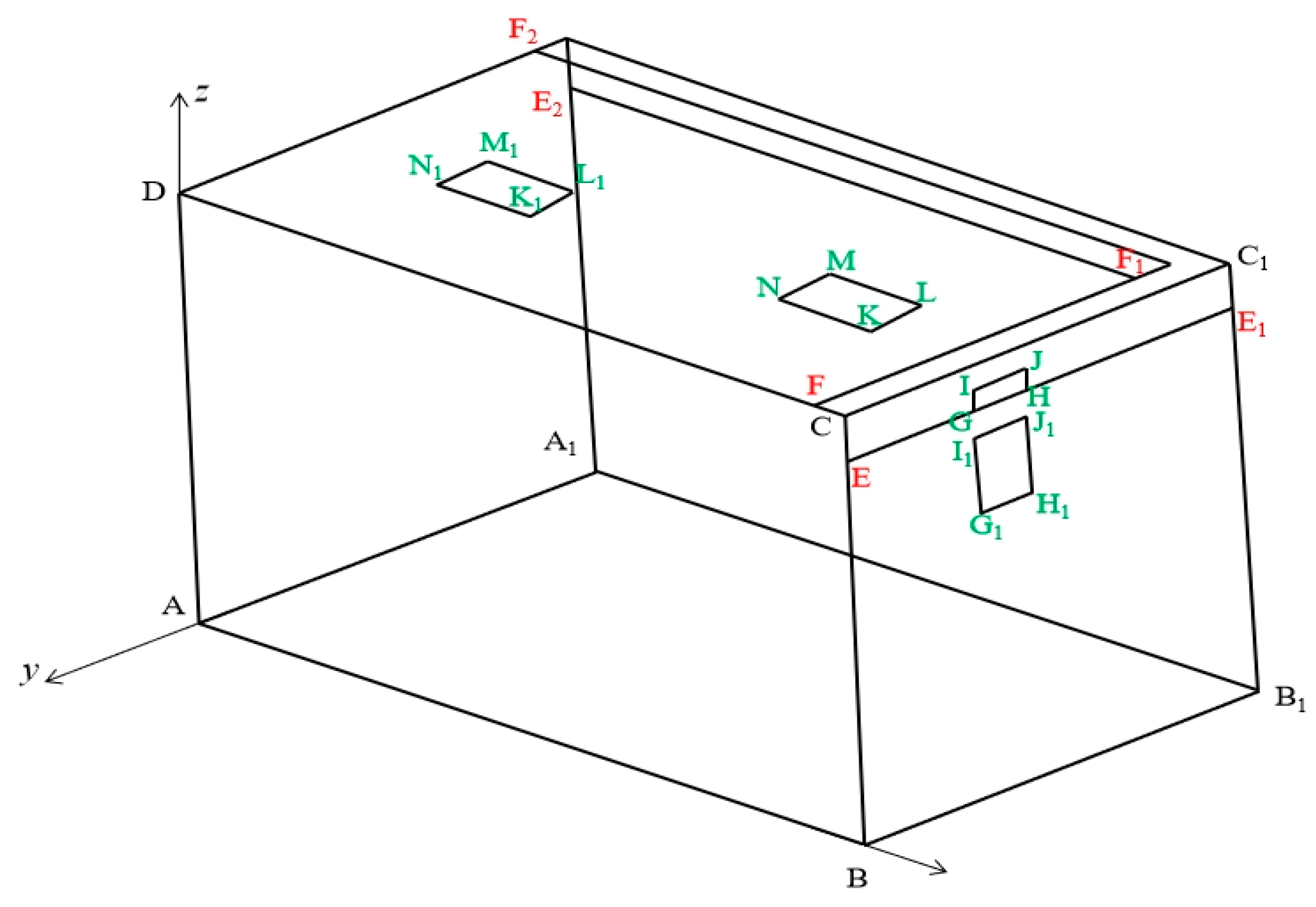
2.1.1. The Shelter’s Geometry

| The Position of Letters (x, y, z) | |||
|---|---|---|---|
| A (0.0000, 0.0000, 0.0000) | B (4.3612, 0.0000, 0.0000) | C (4.3612, 0.0000, 1.8902) | D (0.0000, 0.0000, 1.8902) |
| A1 (0.0000, −2.3711, 0.000) | B1 (4.3612, −2.3711, 0.0000) | C1 (4.3612, −2.3711, 1.8902) | D1 (0.0000, −2.3711, 1.8902) |
| E (4.3612, 0.0000, 1.5921) | E1 (4.3612, −2.3711, 1.5921) | E2 (0.0000, −2.3711, 1.5921) | |
| F (4.1612, 0.0000, 1.8902) | F1 (4.1612, −2.1711, 1.8902) | F2 (0.0000, −2.1711, 1.8902) | |
| G (4.3612, −0.7411, 1.6421) | H (4.3612, −1.0311, 1.6403) | I (4.3612, −0.7411, 1.7221) | J (4.3612, −1.0321, 1.7221) |
| G1 (4.3612, −0.7411, 1.2421) | H1 (4.3612, −1.0311, 1.24) | I1 (4.3612, −0.7411, 1.5721) | J1 (4.3612, −1.0321, 1.5721) |
| K1 (1.4412, −0.7811, 1.8902) | L1 (1.4412, −1.0711, 1.8902) | M1 (0.8121, −1.0711, 1.8902) | N1 (0.8121, −0.7811, 1.8902) |
| K (3.3812, −0.7811, 1.8902) | L (3.3812, −1.0711, 1.8902) | M (2.7512, −1.0711, 1.8902) | N (2.7522, −0.7811, 1.8902) |
- 2.
- 3.
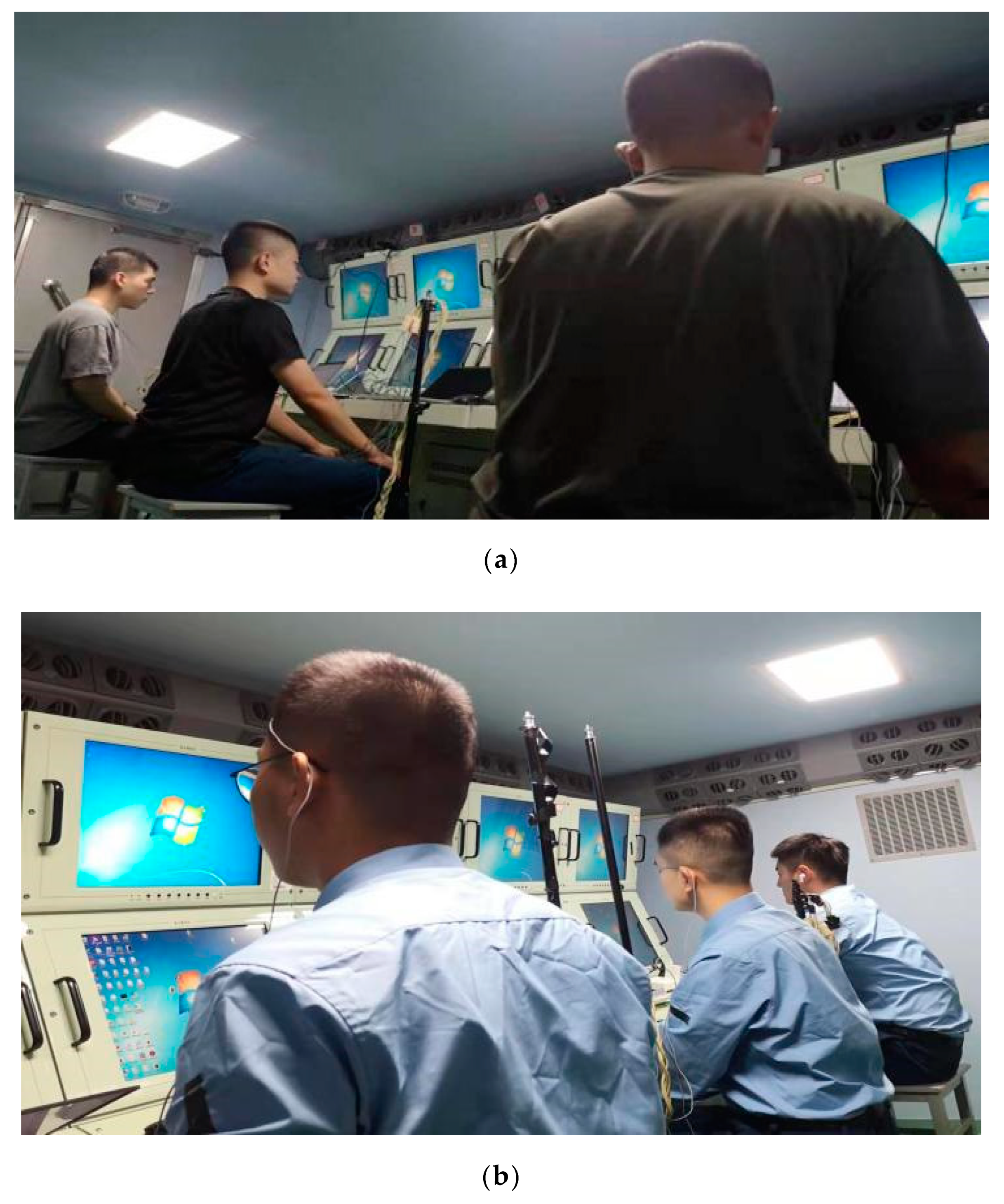
2.1.2. Composition of Subjects
2.1.3. Experimental Conditions
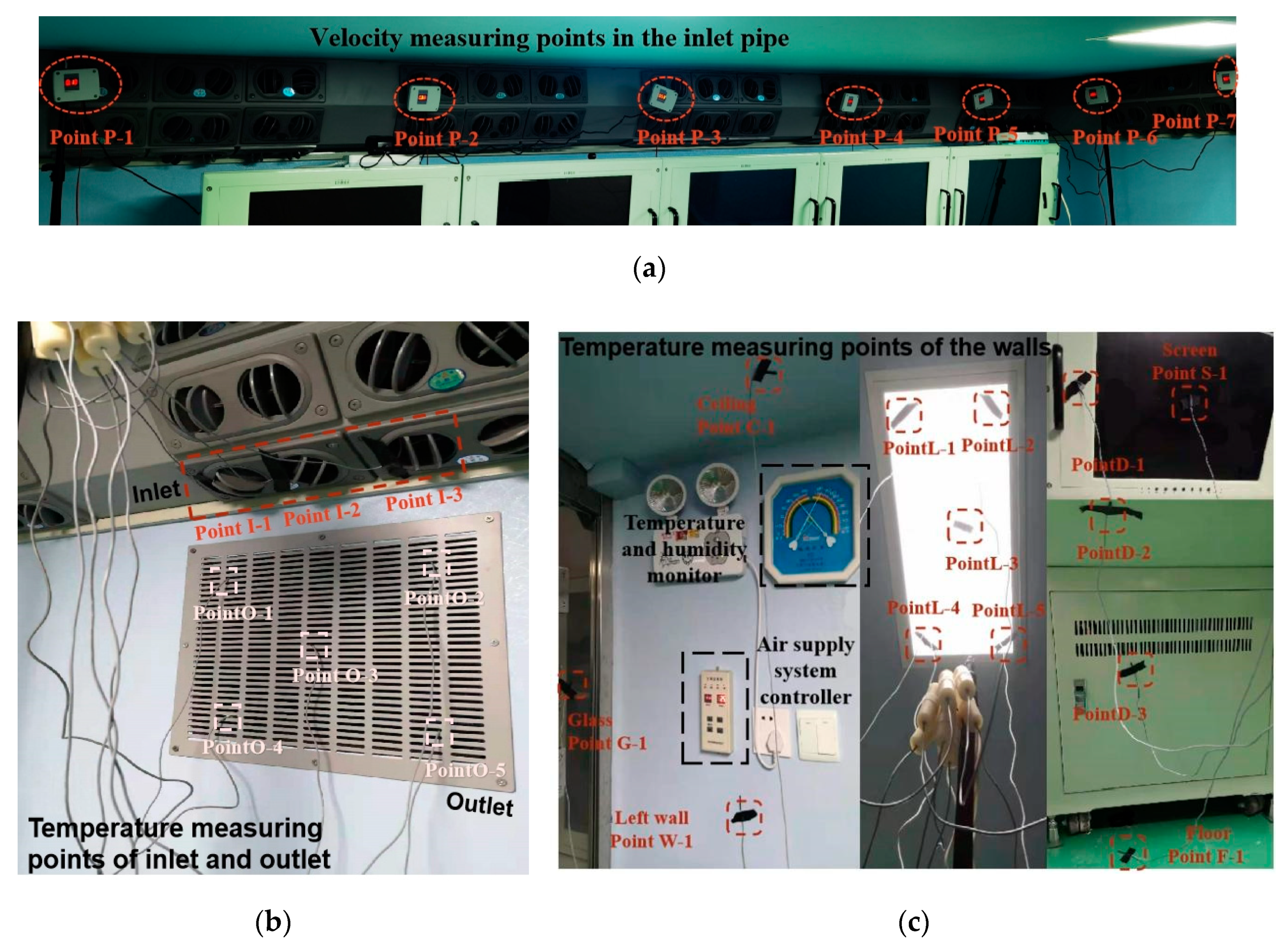
2.2. Location Selection for Sensors in the Shelter
2.2.1. Selection of Measuring Points for the Experiments
- Selection of measuring points for the experiments in the unmanned shelter
- 2.
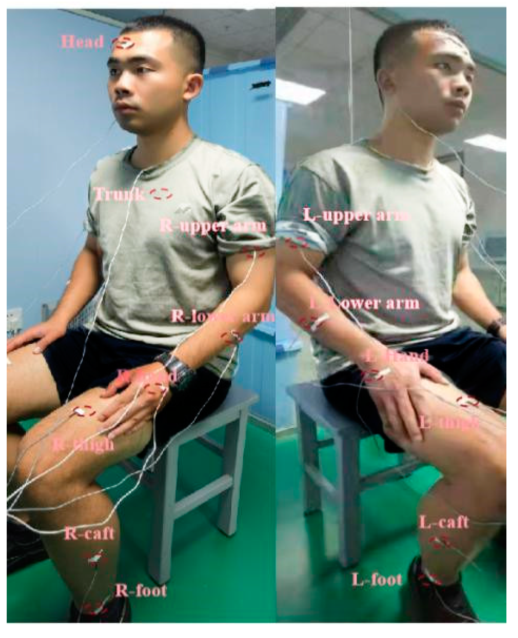
- Selection of measuring points for the manned shelter thermal environment experiment
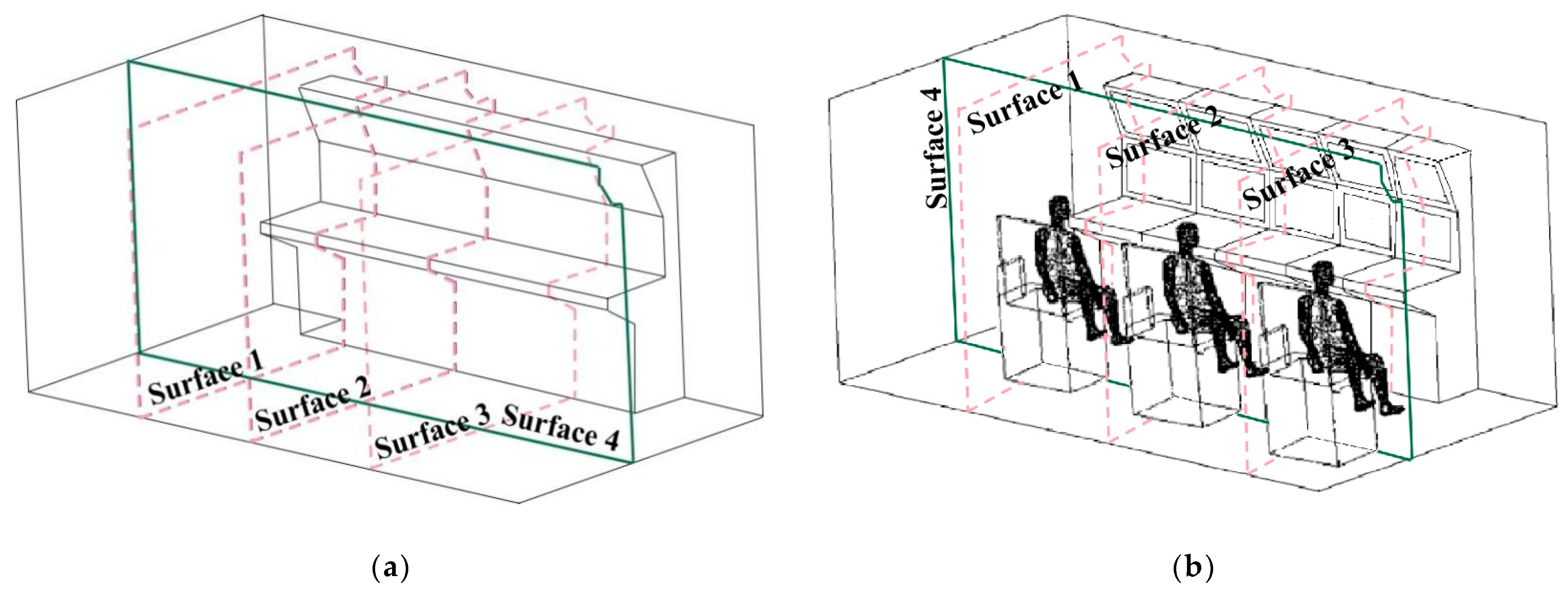
2.2.2. Selection of Measuring Surfaces for Thermal Environment Experiments
2.2.3. The Uncertainties of the Length, Height, and Weight Measurements
- The assessment of measurement uncertainties in length measurements
- 2.
- The assessment of measurement uncertainties in human surface area
3. Data and Processing Analysis
3.1. Temperature Measurement Points Analysis
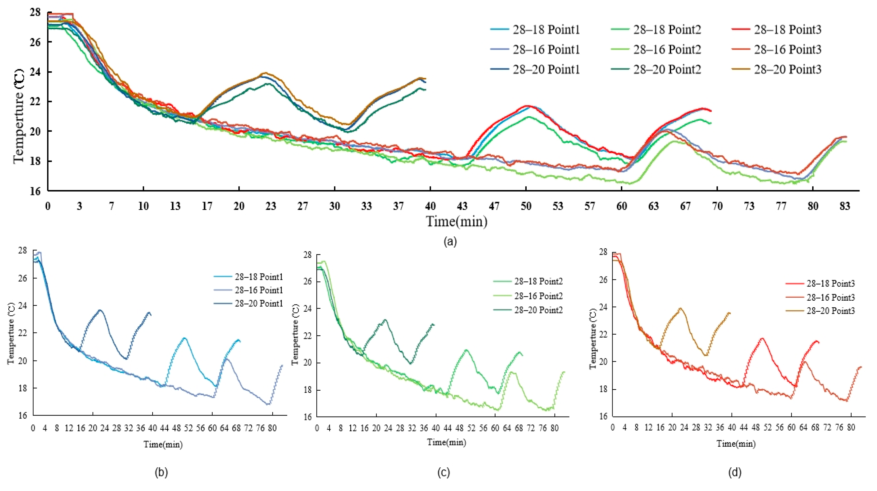
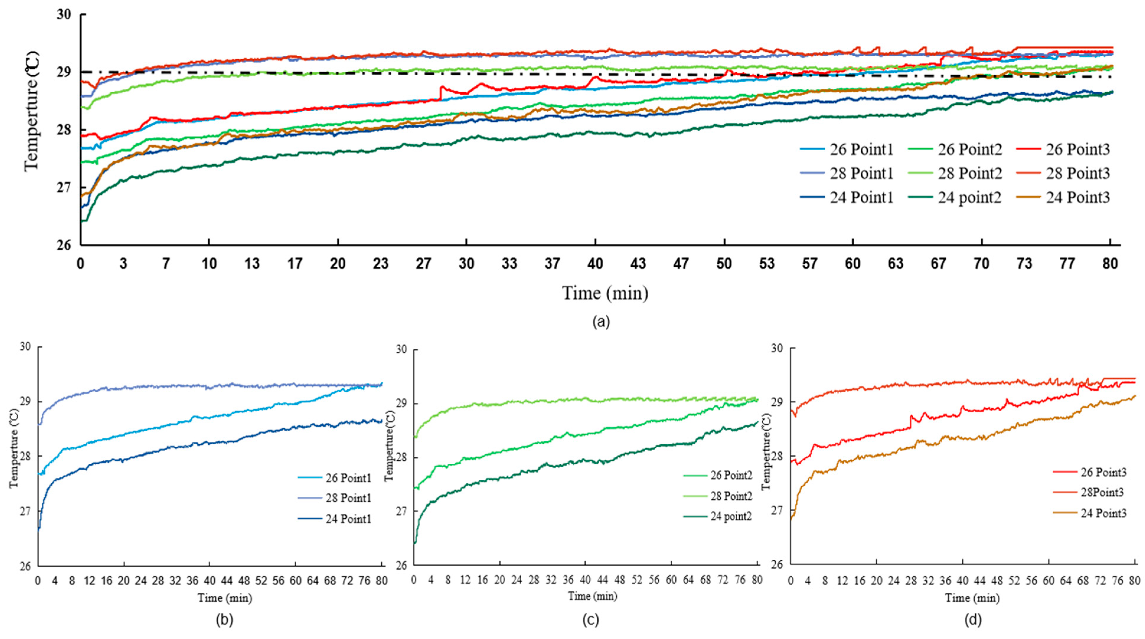
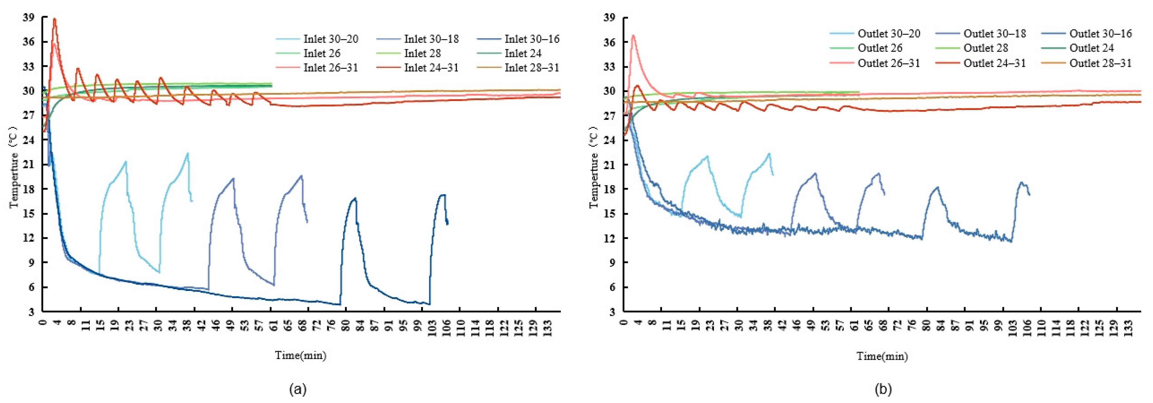
3.1.1. Data Analysis of Temperature Measuring Points in the Shelter
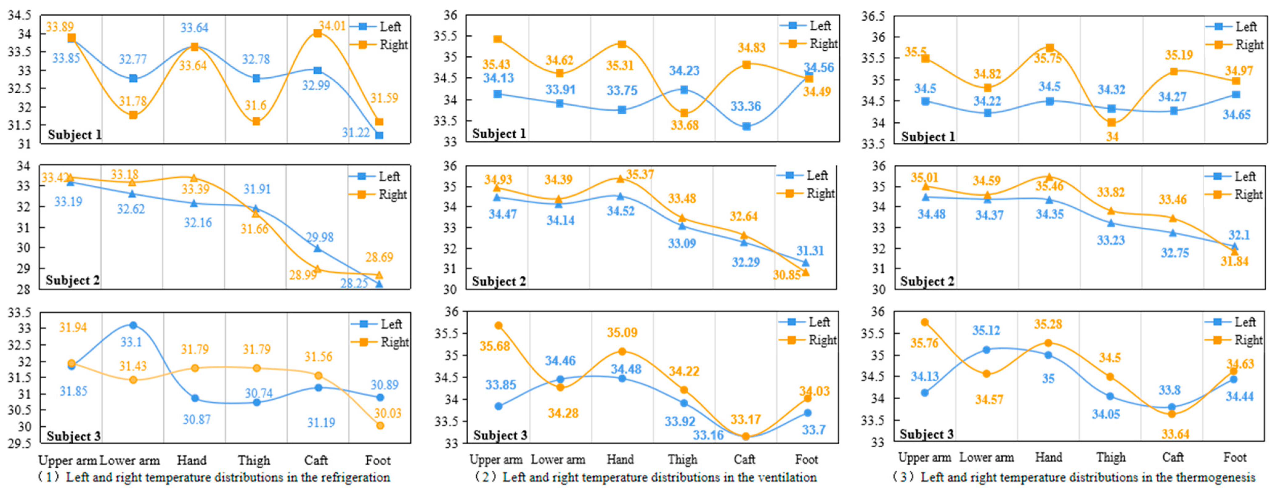
3.1.2. Analysis of Human Body Temperature Distribution
- Data analysis of the Short clothing experiments
- 2.
- Analysis of long clothing experimental data
- 3.
- Analysis of temperature difference of humans wearing different clothes
3.2. Analysis the Wind Speed at the Measuring Points
3.2.1. Distribution of Average Wind Speed at Each Measuring Point of Air Supply Pipeline
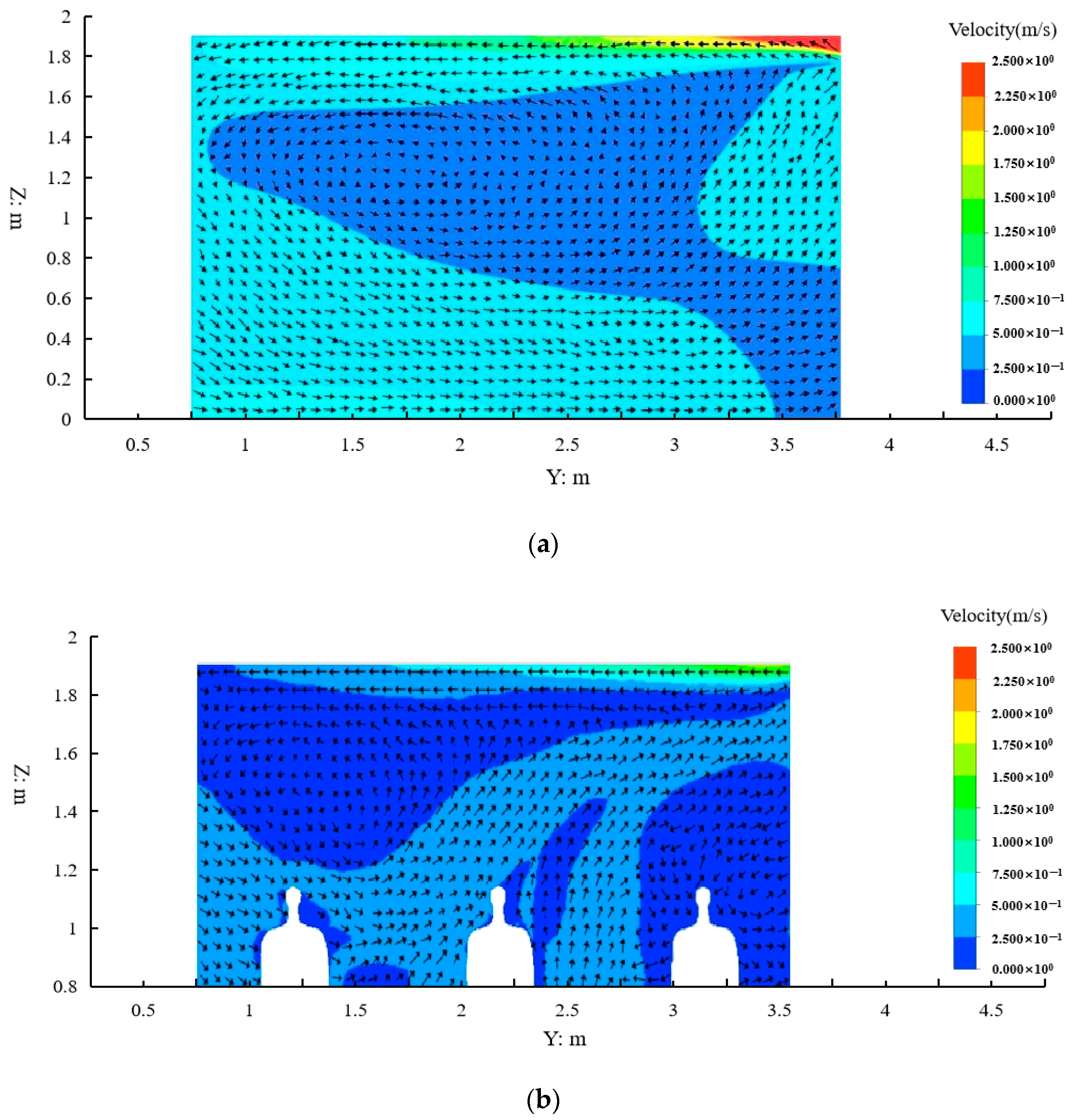
3.2.2. Analysis of Wind Speed Distribution in Special Sections
4. Conclusions
- The measured values of wind velocity and temperature in the experiment can provide experimental verification of initial and wall conditions and simulation results for shelter simulation.
- The function fitted from the experimental data of temperature distribution in the shelter can provide the control equations for the study of air flow temperature control.
- Different wearing conditions, air supply conditions, body part temperatures, and temperature differences between coinciding left and right body parts should be taken into account in a simulation model.
- The thermal plume caused by the vertical temperature difference of the human body has a certain influence on the air distribution in the shelter, which should be paid attention to and taken into account in simulations.
Author Contributions
Funding
Institutional Review Board Statement
Informed Consent Statement
Data Availability Statement
Acknowledgments
Conflicts of Interest
References
- Zhang, M.L.; Jiang, M.; Huang, Y. Simulation Study of Thermal Environment in an Electronic Shelter. Equip. Environ. Eng. 2018, 15, 5–9. [Google Scholar]
- Zhao, W.; Shi, T.; Zhu, C.; Chen, S.; Han, Y. Design of Air Conditioning System for a Radar Cabin Based on Human Thermal Comfort. Electro-Mech. Eng. 2020, 36, 46–49. [Google Scholar]
- Qi, L.; Liu, J.; Zhang, L.; Wu, Q. Study on local thermal sensation and model applicability in vehicle cabin under different driving states. Heat Mass Transf. 2021, 57, 41–52. [Google Scholar] [CrossRef]
- Li, J.; Liu, J.; Dai, S.; Guo, Y.; Jiang, N.; Yang, W. PIV experimental research on gasper jets interacting with the main ventilation in an aircraft cabin. Build. Environ. 2018, 138, 149–159. [Google Scholar] [CrossRef]
- Yang, Z.; Fei, J.; Song, D.; Zhao, Y.; Yu, J.; Yu, X. Effects of simulated natural air movement on thermoregulatory response during head-down bed rest. J. Therm. Biol. 2013, 38, 363–368. [Google Scholar] [CrossRef]
- Gilani, S.; Montazeri, H.; Blocken, B. CFD simulation of stratified indoor environment in displacement ventilation: Validation and sensitivity analysis. Build. Environ. 2016, 95, 299–313. [Google Scholar] [CrossRef]
- Liu, W.; Mazumdar, S.; Zhang, Z.; Poussou, S.B.; Liu, J.; Lin, C.H.; Chen, Q. State-of-the-art methods for studying air distributions in commercial airliner cabins. Build. Environ. 2012, 47, 5–12. [Google Scholar] [CrossRef]
- Fujita, A.; Kanemaru, J.I.; Nakagawa, H.; Ozeki, Y. Numerical simulation method to predict the thermal environment inside a car cabin. JSAE Rev. 2001, 22, 39–47. [Google Scholar] [CrossRef]
- Ware, Y.A.; Khalighi, B. Data-driven prediction of vehicle cabin thermal comfort: Using machine learning and high-fidelity simulation results. Int. J. Heat Mass Transf. 2020, 148, 1–12. [Google Scholar] [CrossRef]
- Zhang, T.F.; Chen, Q. Novel air distribution systems for commercial aircraft cabins. Build. Environ. 2007, 42, 1675–1684. [Google Scholar] [CrossRef]
- Lu, W.; Huang, J.R.; Fan, Y.F.; Zhong, Q. Numerical Model of Flow and Heat Transfer for Manned Spacecraft Pressurized Cabin and Its Ground Verification. J. Astronaut. 2011, 32, 959–965. [Google Scholar]
- Awolesi, S.T.; Awbi, H.B.; Seymour, M.J.; Hiley, R.A. The use of CFD techniques for the assessment and improvement of a workshop ventilation system. In IMechE Seminar on CFD-Tool or Toy; Pergamon Press Ltd.: London, UK, 1991; pp. 39–46. [Google Scholar]
- Zhang, W.; Chen, J.; Lan, F. Experimental study on occupant’s thermal responses under the non-uniform conditions in vehicle cabin during the heating period. Chin. J. Mech. Eng. 2014, 27, 331–339. [Google Scholar] [CrossRef]
- Chai, Y.; Li, W.; Liu, Z. Analysis of transient wave propagation dynamics using the enriched finite element method with interpolation cover functions. Appl. Math. Comput. 2022, 412, 126564. [Google Scholar] [CrossRef]
- Cao, X.; Li, J.; Liu, J.; Yang, W. 2D-PIV measurement of isothermal air jets from a multi-slot diffuser in aircraft cabin environment. Build. Environ. 2016, 99, 44–58. [Google Scholar] [CrossRef]
- Li, J.; Liu, J.; Cao, X.; Jiang, N. Experimental study of transient air distribution of a jet collision region in an aircraft cabin mock-up. Energy Build. 2016, 127, 786–793. [Google Scholar] [CrossRef]
- Li, F.; Liu, J.; Pei, J.; Lin, C.H.; Chen, Q. Experimental study of gaseous and particulate contaminants distribution in an aircraft cabin. Atmos. Environ. 2014, 85, 223–233. [Google Scholar] [CrossRef]
- Li, Z.; Guan, J.; Yang, X.; Lin, C.H. Source apportionment of airborne particles in commercial aircraft cabin environment: Contributions from outside and inside of cabin. Atmos. Environ. 2014, 89, 119–128. [Google Scholar] [CrossRef]
- Zhang, Y.; Liu, J.; Pei, J.; Li, J.; Wang, C. Performance evaluation of different air distribution systems in an aircraft cabin mockup. Aerosp. Sci. Technol. 2017, 70, 359–366. [Google Scholar] [CrossRef]
- Yang, Z.; Fei, J.; Yu, X. Thermal Comfort and Thermoregulation in Manned Space Flight. Chin. J. Appl. Physiol. 2013, 29, 518–524. [Google Scholar]
- Mao, Y.; Wang, J.; Li, J. Experimental and numerical study of air flow and temperature variations in an electric vehicle cabin during refrigeration and heating. Appl. Therm. Eng. 2018, 137, 356–367. [Google Scholar] [CrossRef]
- Aboosaidi, F.; Warfield, M.J.; Choudhury, D. Numerical analysis of airflow in aircraft cabins. In Proceedings of the 21st International Conference on Environmental Systems, San Francisco, CA, USA, 15–18 July 1991; pp. 1441–1446. [Google Scholar]
- Meng, F.; Man, G.; Cao, J. A simplified manned spacecraft cabin air temperature control model and its verification. In Proceedings of the 42nd International Conference on Environmental Systems, San Diego, CA, USA, 15–19 July 2012. [Google Scholar]
- Han, D.; Li, R.; Wang, F.; Sun, Z.; Moon, S.; Gong, Z.; Yu, W.; Zhang, Y. Study on Indoor Thermal Environment Control Based on Thermal Sensation Prediction. Procedia Eng. 2017, 205, 3072–3079. [Google Scholar] [CrossRef]
- Li, Y.; Wei, Q. Simulation of Thermal Environment in Shelter. Electro-Mech. Eng. 2010, 26, 8–9, 21. [Google Scholar]
- Liu, X.H.; Yang, J.Z.; Zhang, Y.T.; Xia, L.N. Simulation Analysis of Thermal Environment in a Radar Shelter. Electro-Mech. Eng. 2012, 28, 8–14. [Google Scholar]
- Li, W.Z. Thermal Design of Electronic Shelter Using ICEPAK Software. Radio Eng. 2011, 41, 55–61. [Google Scholar]
- Mao, Q.J.; Yong-Qing, J.I.; Yun, J.I. Thermal Analysis of Electronic Equipment Shelter. Electro-Mech. Eng. 2014, 30, 24–26. [Google Scholar]
- Pei, D.D. Design Method for Environment Control of Electronic Square Cabin. Movable Power Stn. Veh. 2012, 2, 10–12. [Google Scholar]
- Feng, S.X.; Wang, S.; Yue, W.Q.; Tan, G.B. Research on Heat Transfer Test Method of Shelter. Equip. Environ. Eng. 2011, 8, 109–111. [Google Scholar]
- Liao, C.Y.; Chen, S.L.; Chou, T.D.; Lee, T.P.; Dai, N.T.; Chen, T.M. Use of two-dimensional projection for estimating hand surface area of Chinese adults. Burns 2008, 34, 556–559. [Google Scholar] [CrossRef]
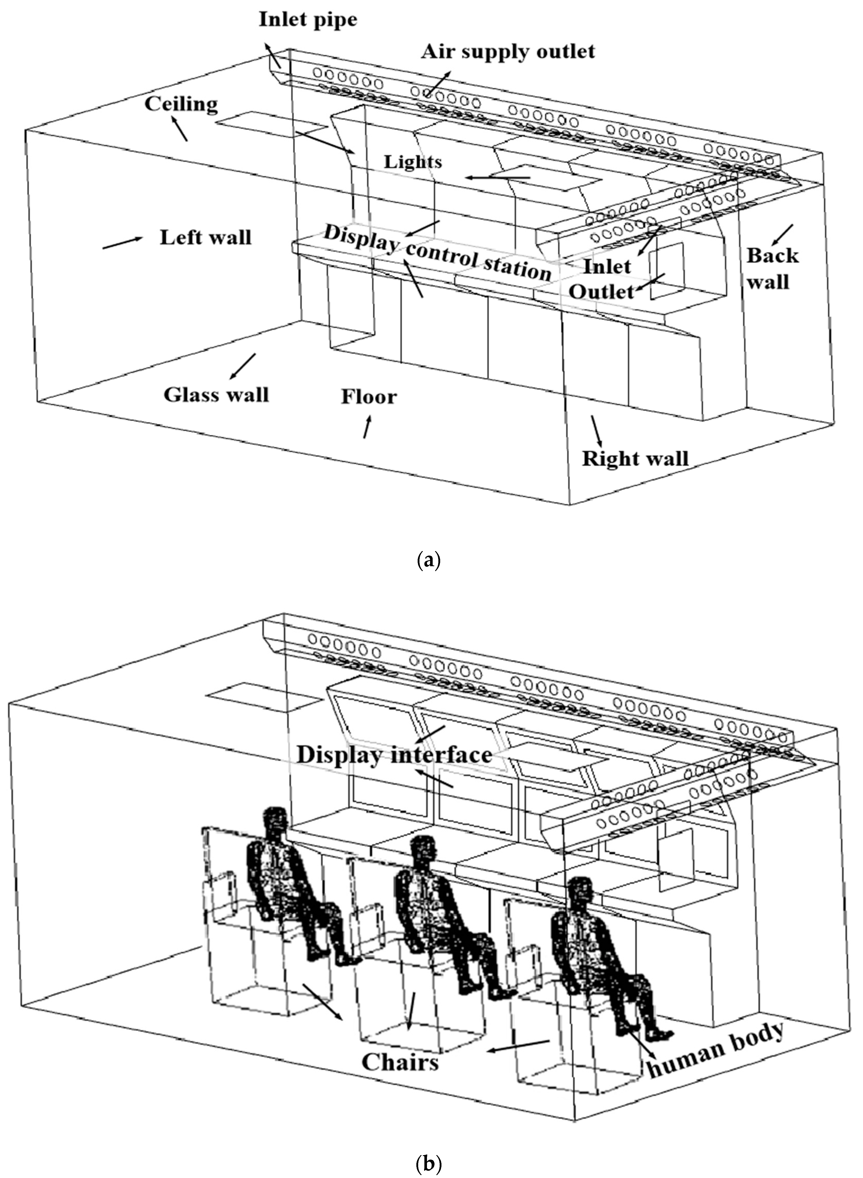


| Name | Size (m) | Number | Monitoring Mode (Number of Points) | Equipment |
|---|---|---|---|---|
| Inlet pipe | X: 4.360 (length) × 0.200 × 0.300 Y: 2.370 × 0.200 × 0.300 | 1 | Points (7 × 1) | Pipe wind meter |
| Air supply outlet | R: 0.630 | 126 | Open or Close | |
| Ceiling | 4.360 (length) × 2.370 (width) | 1 | Points (5 × 1) | Temperature sensor |
| Lights | 0.630 × 0.286 | 2 | Points (5 × 2) | |
| Display control station | 1.600 × 0.400 × 0.600 | 5 | Points (7 × 5) | |
| Inlet | 0.290 × 0.080 | 1 | Points (3 × 1) | |
| Outlet | 0.330 × 0.290 | 1 | Points (5 × 1) | |
| Glass Wall | 4.36 × 1.89 | 1 | Points (5 × 1) | |
| Wall | Left/Right: 2.370 × 1.890 Back: 4.360 × 1.890 | 3 | Points (5 × 3) | |
| Floor | 4.360 (length) × 2.370 (width) | 1 | Points (5 × 1) | |
| Display interface | 0.800 × 0.600 | 10 | Points (5 × 10) | |
| Human body | H: 1.700~1.850 | 3 | Surfaces (5 × 1) | PIV Measuring wind speed |
| chairs | 0.477 × 0.477 × 0.800 | 3 | Surfaces (5 × 1) |
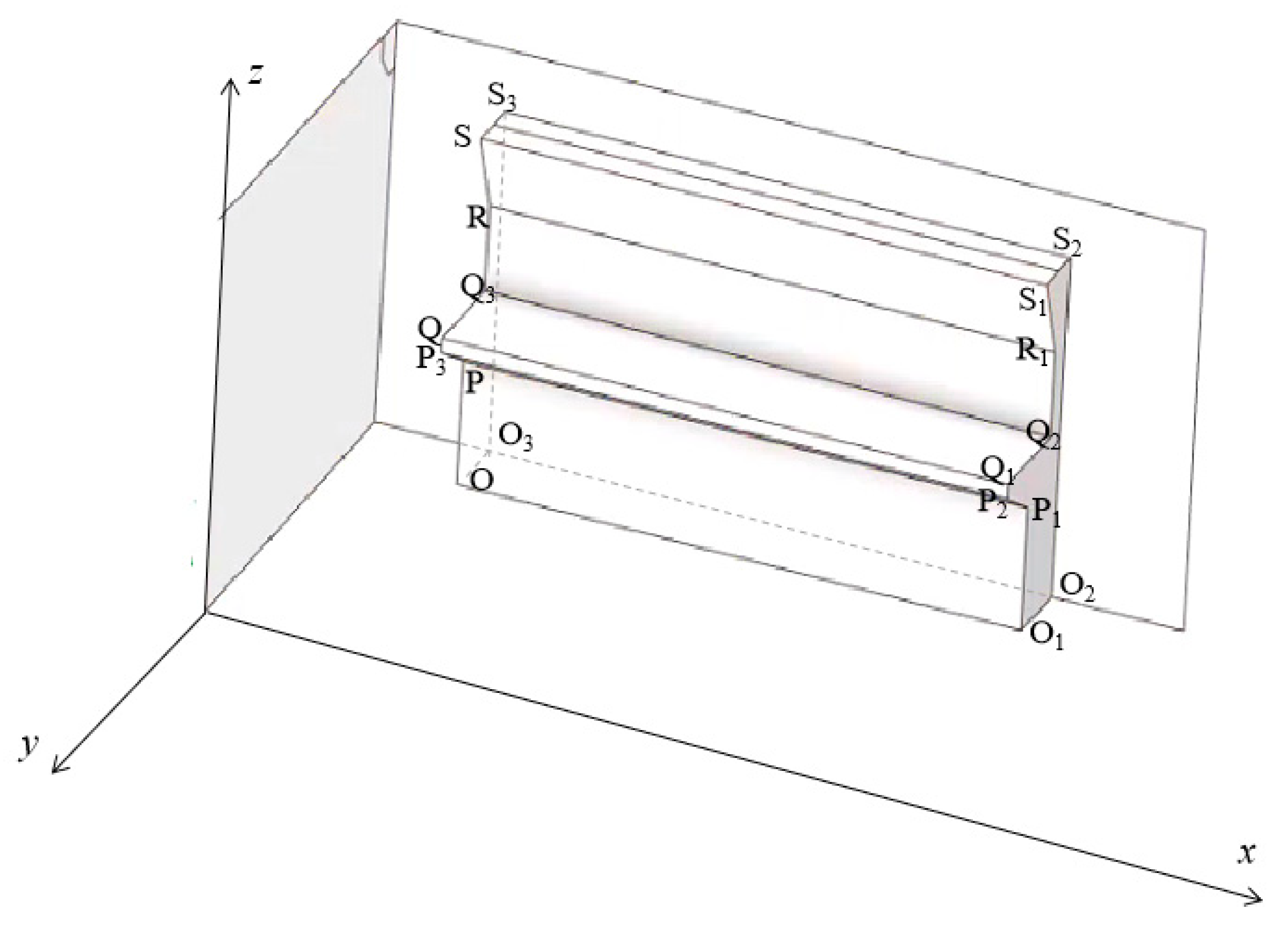
| The Position of Letters (x, y, z) | |||
|---|---|---|---|
| O (0.6413, −1.7432, 0.0000) | O1 (3.6421, −1.7432, 0.0000) | O2 (3.6421, −2.3722, 0.0000) | O3 (0.6412, −2.3722, 0.0000) |
| P (0.6413, −1.7432, 0.6713) | P1 (3.6421, −1.7432, 0.6713) | P2 (3.6421, −1.4351, 0.7620) | P3 (0.6412, −1.43531, 0.7620) |
| Q (0.6413, −1.4353, 0.8213) | Q1 (3.6421, −1.4351, 0.8213) | Q2 (3.6421, −1.9121, 0.8112) | Q3 (0.6412, −1.9121, 0.8246) |
| R (0.6413, −1.9121, 1.2133) | R1 (3.6421, −1.9121, 1.2133) | ||
| S (0.6413, −2.0403, 1.6213) | S1 (3.6421, −2.0403, 1.6213) | S2 (3.6421, −2.3732, 1.6221) | S3 (0.6412, −2.3722, 1.6221) |
| The Position of Letters (x, y, z) | ||
|---|---|---|
| E (4.3602, 0.0000, 1.5922) | E1 (4.3602, −2.3723, 1.5922) | E2 (0.0000, −2.3723, 1.5922) |
| F (4.1603, 0.0000, 1.8912) | F1 (4.1603, −2.1716, 1.8912) | F2 (0.0000, −2.1716, 1.8912) |
| U (4.1603, 0.0000, 1.7821) | U1 (4.1603, −2.1716, 1.7821) | U2 (0.0000, −2.1716, 1.7821) |
| T (4.2621, 0.0000, 1.5923) | T1 (4.2621, −2.2702, 1.5923) | T2 (0.0000, −2.2702, 1.5923) |
| Group | Height (cm) | Weight (kg) | Age | Exercise Time (hour) | Surface Area (m2) | Dress | |
|---|---|---|---|---|---|---|---|
| 1 | A | 1.742 | 70.2 | 22 | 1 | 1.8754 | Short sleeves and shorts |
| B | 1.823 | 73.3 | 22 | 1 | 1.9621 | ||
| C | 1.701 | 71.4 | 21 | 1 | 1.8638 | ||
| 2 | A | 1.698 | 73.2 | 26 | 1.5 | 1.8831 | Long sleeves and pants |
| B | 1.742 | 70.6 | 23 | 1.5 | 1.8754 | ||
| C | 1.702 | 67.1 | 26 | 1.5 | 1.8130 | ||
| 3 | A | 1.751 | 65.5 | 25 | 1 | 1.8179 | Short sleeves and shorts |
| B | 1.723 | 68.3 | 25 | 1 | 1.8378 | ||
| C | 1.701 | 62.2 | 21 | 1 | 1.7495 | ||
| 4 | A | 1.703 | 64.7 | 22 | 1 | 1.7749 | Long sleeves and pants |
| B | 1.842 | 75.3 | 20 | 1.5 | 1.9996 | ||
| C | 1.811 | 76.1 | 21 | 1 | 1.9941 | ||
| 5 | A | 1.823 | 79.8 | 20 | 1.5 | 2.0382 | Shorty/Long sleeves and pants |
| B | 1.751 | 66.2 | 20 | 1.5 | 1.8307 | ||
| C | 1.832 | 77.1 | 20 | 1.5 | 2.0189 | ||
| 6 | A | 1.703 | 76.3 | 25 | 1.5 | 1.9273 | Long sleeves and pants |
| B | 1.782 | 76.2 | 20 | 2 | 1.9759 | ||
| C | 1.721 | 68.1 | 21 | 2 | 1.8378 | ||
| 7 | A | 1.833 | 72.3 | 21 | 1.5 | 1.9554 | Short sleeves and shorts |
| B | 1.752 | 71.1 | 21 | 1.5 | 1.8942 | ||
| C | 1.784 | 70.2 | 22 | 1.5 | 1.8997 | ||
| 8 | A | 1.742 | 60.1 | 22 | 1 | 1.7484 | Shorty/Long sleeves and pants |
| B | 1.843 | 83.4 | 25 | 1 | 2.1012 | ||
| C | 1.824 | 75.2 | 22 | 1 | 1.9874 | ||
| 9 | A | 1.712 | 61.1 | 21 | 1 | 1.7429 | Long sleeves and pants |
| B | 1.883 | 89.5 | 23 | 1 | 2.2017 | ||
| C | 1.752 | 70.3 | 24 | 1 | 1.8815 | ||
| 10 | A | 1.724 | 65.1 | 23 | 0.5 | 1.7998 | Short sleeves and shorts |
| B | 1.683 | 65.2 | 23 | 0.5 | 1.7755 | ||
| C | 1.811 | 77.3 | 23 | 1 | 2.0068 | ||
| Refrigeration Condition | Ventilation Condition | Heating Conditions |
|---|---|---|
| Case 1: 28–16 °C | Case 4: 24–30 °C | Case 7: 24–31 °C |
| Case 2: 28–18 °C | Case 5: 26–30 °C | Case 8: 26–31 °C |
| Case 3: 28–20 °C | Case 6: 28–30 °C | Case 9: 28–31 °C |
| Coordinates of Different Measuring Points in Each Equipment (x, y, z) | |
|---|---|
| Point P | 1 (0.37, −2.17, 1.83), 2 (1.17, −2.17, 1.83), 3 (1.97, −2.17, 1.83), 4 (2.77, −2.17, 1.83), 5 (3.57, −2.17, 1.83) 6 (4.16, −1.77, 1.83), 7 (0.97, −0.97, 1.83) |
| Point I | 1 (4.31, −0.99, 1.59), 2 (4.31, −0.89, 1.59), 3 (4.31, −0.79, 1.59) |
| Point O | 1 (4.36, −1.05, 1.50), 2 (4.36, −0.82, 1.50), 3 (4.36, −0.92, 1.38), 4 (4.36, −1.05, 1.26), 5 (4.36, −0.82, 1.26) |
| Point C | 1 (0.68, −0.45, 1.89), 2 (0.68, −1.92, 1.89), 3 (2.29, −1.18, 1.89), 4 (3.91, −0.45, 1.89), 5 (3.91, −1.92, 1.89) |
| Point G | 1 (0.68, 0, 1.44), 2 (0.68, 0, 0.45), 3 (2.29, 0, 0.95), 4 (3.91, −0, 1.44), 5 (3.91, 0, 0.45) |
| Point W | 1 (0, −0.45, 1.44), 2 (0, −1.92, 1.44), 3 (0, −1.18, 0.95), 4 (0, −0.45, 0.45), 5 (0, −1.92, 0.45) 6 (0.68, −2.37, 1.44), 7 (0.68, −2.37, 0.45), 8 (2.29, −2.37, 0.95), 9 (3.91, −2.37, 1.44), 10 (3.91, −2.37, 0.45) 11 (4.36, −0.45, 1.44), 12 (4.36, −1.92, 1.44), 13 (4.36, −1.18, 0.95), 14 (4.36, −0.45, 0.45), 15 (4.36, −1.92, 0.45) |
| Point L | 1 (0.9, −0.88, 1.89), 2 (0.9, −1.08, 1.89), 3 (1.13, −0.98, 1.89), 4 (1.36, −0.88, 1.89), 5 (1.36, −1.08, 0.1.89) 6 (3.46, −0.88, 1.89), 7 (3.46, −1.08, 1.89), 8 (3.23, −0.98, 1.89), 9 (3, −0.88, 1.89), 10 (3, −1.08, 0.1.89) |
| Point S | 1 (0.95, −2.06, 1.36), 2 (1.55, −2.06, 1.36), 3 (2.15, −2.06, 1.36), 4 (2.75, −2.06, 1.36), 5 (3.35, −2.06, 1.36) 6 (0.95, −2.11, 1.01), 7 (1.55, −2.11, 1.01), 8 ( (2.15, −2.11, 1.01), 9 (2.75, −2.11, 1.01), 10 (3.35, −2.11, 1.01) |
| Point D | 1 (0.69, −2.06, 1.36), 2 (1.29, −2.06, 1.36), 3 (1.89, −2.06, 1.36), 4 (2.49, −2.06, 1.36), 5 (3.09, −2.06, 1.36) 6 (0.69, −2.11, 1.01), 7 (1.29, −2.11, 1.01), 8 (1.89, −2.11, 1.01), 9 (2.49, −2.11, 1.01), 10 (3.09, −2.11, 1.01) 1 (0.95, −1.59, 0.67), 2 (1.55, −1.59, 0.67), 3 (2.15, −1.59, 0.67), 4 (2.75, −1.59, 0.67), 5 (3.35, −1.59, 0.67) 6 (0.95, −1.74, 0.34), 7 (1.55, −1.74, 0.34), 8 ( (2.15, −1.74, 0.34), 9 (2.75, −1.74, 0.34), 10 (3.35, −1.74, 0.34) |
| Point F | 1 (0.45, −0.45, 0), 2 (0.45, −1.92, 0), 3 (2.18, −1.19, 0), 4 (3.91, −1.19, 0), 5 (3.91, −1.92, 0) |
| Point R | 1 (1.24, −1.12, 0.56), 2 (2.14, −1.12, 0.56), 3 (3.04, −1.12, 0.56) |
| The Temperature of the Room (℃) | Temperature 24 | Temperature 26 | Temperature 28 |
|---|---|---|---|
| Left wall measurement temperature (°C) | 26.710 | 27.061 | 28.712 |
| Right wall measurement temperature (°C) | 26.801 | 27.473 | 29.459 |
| Back wall measurement temperature (°C) | 26.811 | 26.811 | 29.616 |
| Glass wall measurement temperature (°C) | 26.802 | 26.291 | 28.886 |
| Floor wall measurement temperature (°C) | 25.502 | 27.402 | 28.916 |
| Light measurement temperature (°C) | 33.554 | 33.884 | 33.779 |
| Ceiling measurement temperature (°C) | 27.571 | 27.001 | 29.773 |
| Display control station temperature (°C) | 28.863 | 29.342 | 32.117 |
| 27.822 | 28.552 | 31.529 | |
| 27.142 | 27.634 | 30.397 | |
| 26.091 | 26.406 | 29.521 | |
| Chair measurement temperature (°C) (Human body) | 31.201 | 31.804 | 32.002 |
| Display interface temperature (Human body) | 33.093 | 33.233 | 33.423 |
| Case | Coefficients | Points | Polynomial Coefficients | |||||||||||
|---|---|---|---|---|---|---|---|---|---|---|---|---|---|---|
| a | b | c | A | B1 | B2 | B3 | B4 | B5 | B6 | B7 | B8 | B9 | ||
| Case 1 | 27.72 | 2.52 | 0.62 | 1 | 1.15 × 10⁷ | −1.29 × 10⁶ | 6.34 × 10⁴ | −1.77 × 10³ | 30.63 | −0.34 | 0.23 × 10⁻² | −9.05 × 10⁻⁶ | 1.53 × 10⁻⁸ | −5.1 |
| 2 | −1.22 × 10⁸ | 1.62 × 10⁷ | −9.56 × 10⁵ | 3.27 × 10⁴ | −716.67 | 10.44 | −0.1 | 6.26 × 10⁻⁴ | −2.26 × 10⁻⁶ | 3.61 × 10⁻⁹ | ||||
| 3 | −8.73 × 10⁷ | 1.16 × 10⁷ | −6.87 × 10⁵ | 2.36 × 10⁴ | −518.8 | 7.58 | −0.07 | 4.57 × 10⁻⁴ | −1.65 × 10⁻⁶ | 2.65 × 10⁻⁹ | ||||
| Case 2 | 27.84 | 2.75 | 0.74 | 1 | −1.49 × 10⁴ | 2604.26 | −178.95 | 6.44 | −0.13 | 1.6 × 10⁻³ | −1.04 × 10⁻⁵ | 2.08 × 10⁻⁸ | - | - |
| 2 | 3.51 × 10⁴ | −3.92 × 10³ | 184.16 | −4.71 | 0.071 | −6.34 × 10⁻⁴ | 3.12 × 10⁻⁶ | −6.55 × 10⁻⁹ | - | - | ||||
| 3 | −8.58 × 10⁴ | 1.14 × 10⁴ | −646.69 | 20.18 | −0.37 | 4.1 × 10³ | −2.51 × 10⁻⁵ | 6.49 × 10⁻⁸ | - | - | ||||
| Case 3 | 27.13 | 2.75 | 0.63 | 1 | 284.56 | −61.01 | 5.38 | −0.23 | 0.045 | −3.49 × 10⁻⁵ | - | - | - | - |
| 2 | 266.21 | −56.25 | 4.93 | −0.21 | 4.1 × 10⁻³ | −3.18 × 10⁻⁵ | - | - | - | - | ||||
| 3 | 268.84 | −58.73 | 5.28 | −0.22 | 4.6 × 10⁻³ | −3.56 × 10⁻⁵ | - | - | - | - | ||||
| Case 4 | - | - | - | 1 | 27.65 | 0.15 | −0.019 | 1.46 × 10⁻³ | −6.87 × 10⁻⁵ | 2.01 × 10⁻⁶ | −3.68 × 10⁻⁸ | 4.08 × 10⁻¹⁰ | −2.50 × 10⁻¹² | 6.48 × 10⁻¹⁵ |
| 2 | 27.35 | 0.13 | −0.013 | 8.8 × 10⁻⁴ | −3.67 × 10⁻⁵ | 9.99 × 10⁻⁷ | −1.79 × 10⁻⁸ | 2.01 × 10⁻¹⁰ | −1.28 × 10⁻¹² | 3.48 × 10⁻¹⁵ | ||||
| 3 | 27.84 | 0.028 | 7.4 × 10⁻³ | −1.24 × 10⁻³ | 8.36 × 10⁻⁵ | −2.96 × 10⁻⁶ | 5.99 × 10⁻⁸ | −6.98 × 10⁻¹⁰ | 4.37 × 10⁻¹² | −1.14 × 10⁻¹⁴ | ||||
| Case 5 | - | - | - | 1 | 28.54 | 0.16 | −0.0197 | 1.43 × 10⁻³ | −6.29 × 10⁻⁵ | 1.73 × 10⁻⁶ | −2.99 × 10⁻⁸ | 3.15 × 10⁻¹⁰ | −1.85 × 10⁻¹² | 4.64 × 10⁻¹⁵ |
| 2 | 28.34 | 0.14 | −0.0148 | 9.2 × 10⁻⁴ | −3.61 × 10⁻⁵ | 9.12 × 10⁻⁷ | −1.49 × 10⁻⁸ | 1.53 × 10⁻¹⁰ | −8.83 × 10⁻¹³ | 2.20 × 10⁻¹⁵ | ||||
| 3 | 28.75 | 0.082 | −0.0055 | 1.7 × 10⁻⁴ | −2.57 × 10⁻⁷ | −1.23 × 10⁻⁷ | 3.46 × 10⁻⁹ | −4.26 × 10⁻¹¹ | 2.48 × 10⁻¹³ | −5.31 × 10⁻¹⁶ | ||||
| Case 6 | - | - | - | 1 | 26.68 | 0.36 | −0.051 | 3.9 × 10⁻³ | −1.7 × 10⁻⁴ | 4.44 × 10⁻⁶ | −7.15 × 10⁻⁸ | 6.91 × 10⁻¹⁰ | −3.67 × 10⁻¹² | 8.22 × 10⁻¹⁵ |
| 2 | 26.41 | 0.32 | −0.045 | 3.7 × 10⁻³ | −1.7 × 10⁻⁴ | 5.03 × 10⁻⁶ | −8.94 × 10⁻⁸ | 9.61 × 10⁻¹⁰ | −5.72 × 10⁻¹² | 1.45 × 10⁻¹⁴ | ||||
| 3 | 26.78 | 0.31 | −0.041 | 3.01 × 10⁻³ | −0.1 × 10⁻³ | 3.31 × 10⁻⁶ | −5.28 × 10⁻⁸ | 5.08 × 10⁻¹⁰ | −2.71 × 10⁻¹² | 6.15 × 10⁻¹⁵ | ||||
| Case 7 | 0.09 | 6.11 × 10126 | 3.17 | 1 | 23.80 | 1.13 | −3.03 | 3.72 | −2.12 | 0.69 | −0.14 | 1.58 × 10⁻² | −9.94 × 10⁻⁴ | 2.60 × 10⁻⁵ |
| 27.67 | 0.012 | 1.63 × 10⁻⁴ | −1.77 × 10⁻⁶ | - | - | - | - | - | - | |||||
| 0.08 | 5.11 × 10126 | 3.15 | 2 | 23.37 | 0.64 | −1.71 | 2.32 | −1.38 | 0.47 | −9.66 × 10⁻² | 1.17 × 10⁻² | −7.62 × 10⁻⁴ | 2.07 × 10⁻⁵ | |
| 27.28 | 0.015 | 6.11 × 10⁻⁵ | −1.04 × 10⁻⁶ | - | - | - | - | - | - | |||||
| 0.07 | 6.27 × 10127 | 3.17 | 3 | 23.47 | 1.34 | −4.46 | 6.30 | −4.24 | 1.61 | −0.36 | 4.70 × 10⁻² | −3.32 × 10⁻³ | 9.80 × 10⁻⁵ | |
| 27.09 | 6.54 × 10⁻³ | 3.71 × 10⁻⁴ | −3.30 × 10⁻⁶ | - | - | - | - | - | - | |||||
| Case 8 | 27.29 | 0.0073 | 1 | 25.96 | −3.53 × 10⁻³ | −0.17 | 0.32 | −0.11 | 0.018 | −1.51 × 10⁻³ | 6.43 × 10⁻⁵ | −1.10 × 10⁻⁶ | - | |
| 27.01 | 0.0074 | 2 | 25.71 | 0.10 | −0.45 | 0.49 | −0.16 | 0.026 | −2.19 × 10⁻³ | 9.36 × 10⁻⁵ | −1.62 × 10⁻⁶ | - | ||
| 27.29 | 0.0076 | 3 | 26.16 | 0.096 | −0.35 | 0.35 | −0.11 | 0.017 | −1.43 × 10⁻³ | 6.08 × 10⁻⁵ | −1.05 × 10⁻⁶ | - | ||
| Case 9 | 28.74 | 0.0067 | 1 | - | - | - | - | - | - | - | - | - | - | |
| 28.33 | 0.0074 | 2 | - | - | - | - | - | - | - | - | - | - | ||
| 28.29 | 0.0068 | 3 | - | - | - | - | - | - | - | - | - | - | ||
Publisher’s Note: MDPI stays neutral with regard to jurisdictional claims in published maps and institutional affiliations. |
© 2022 by the authors. Licensee MDPI, Basel, Switzerland. This article is an open access article distributed under the terms and conditions of the Creative Commons Attribution (CC BY) license (https://creativecommons.org/licenses/by/4.0/).
Share and Cite
Qu, J.; Guo, H.; Xue, H.; Dang, S.; Chen, Y. Experimental Study on Manned/Unmanned Thermal Environment in Radar Electronic Shelter Based on Different Air Supply Conditions. Energies 2022, 15, 1277. https://doi.org/10.3390/en15041277
Qu J, Guo H, Xue H, Dang S, Chen Y. Experimental Study on Manned/Unmanned Thermal Environment in Radar Electronic Shelter Based on Different Air Supply Conditions. Energies. 2022; 15(4):1277. https://doi.org/10.3390/en15041277
Chicago/Turabian StyleQu, Jue, Hao Guo, Hongjun Xue, Sina Dang, and Yingchun Chen. 2022. "Experimental Study on Manned/Unmanned Thermal Environment in Radar Electronic Shelter Based on Different Air Supply Conditions" Energies 15, no. 4: 1277. https://doi.org/10.3390/en15041277