Hybrid Research Platform for Fundamental and Empirical Modeling and Analysis of Energy Management of Shared Electric Vehicles

Abstract

This article presents the results of the development of a hybrid research platform for fundamental and empirical modeling and analysis of energy management of shared electric vehicles. The article describes the hybrid model and its specific features in detail. Within the model architecture, a part of the fundamental model, empirical model and data collection tools were interconnected. The uniqueness lies in the models of electric cars created for a specific vehicle using cost-optimal parameterizations, as well as the implementation of a cloud solution, which is based on custom data communication, custom data logger and cost-optimized parameterization of machine learning algorithms. Experimental verification was performed on a real electric car in public traffic. The car is part of casharing platform.

1. Introduction

In conventional automobiles, consumption is measured by litres of gasoline per 100 km. In the new, electric era, consumption is expressed in kWh. According to [1], the consumption of a modern, electric automobile listed by the manufacturer begins at 15 kWh/100 km. These measurements take place under precisely defined conditions using driving cycles.

There are a number of consumption prediction models for determining the range of electric vehicles [2,3]. The first group includes empirical models, including regression, statistical models, machine learning models, state space models, etc., which all use long-term driving data analysis and are isolated from the physical laws of vehicle dynamics. However, this information is inherently included in the data. The advantage of such models is the elimination of a mathematical description of individual components of the vehicle affecting consumption, such as the parameters of the electric motor or battery, which can only be determined with certainty using special measurements or estimates from available literature. Another advantage lies in the data itself, which contains difficult-to-predict factors of real conditions such as the influence of weather (i.e., temperature, wind speed and amount of precipitation), traffic density, driving style, additional features, etc. With the growing amount of data, the accuracy of the prediction increases, but so does its significant volume. On the contrary, the disadvantage is the duration and infrastructure needed to collect such travel data. An example of empirical modeling for deriving a behavioral behavior model and driving prediction for PHEV (Plug-in Hybrid Electric Vehicle) is in [4]. In the first step, a model of the driver’s behavior in a given traffic situation environment is created. In the second step, the off-line classification of the driver’s driving style is performed using K-means clustering, i.e., from the data entered before the ride itself. Refinement is achieved through online classification using neural networks, i.e., from data obtained while driving. Finally, the models are linked to obtain the best fuel economy optimization strategy. Another model is described in [5], where there is a design of an off-line driving assistant, and where the results of the ride are only available at the end of the ride. The assistant is based on the collection and analysis of data on weather, route geometry, driving style and traffic situation. This data is analyzed using three artificial intelligence methods-linear regression, decision trees and neural networks. The off-line driving analysis is available on the web interface. Another approach is in [6,7], where a smartphone with Android OS is used to collect real data from the car via an OBD-Bluetooth adapter. Here, GPS data, weather information, etc. are used in addition to telemetry. The research deals with driving style classification using J48, Naïve Bayes and Random Forest machine learning algorithms running in real time on a smartphone. Drivers are given suggestions (in the form of gamification) on how to adjust their driving style to achieve the lowest possible consumption. From the same authors, the system is improved [8] using data from a smartphone camera, which allows the detection of accidents and traffic lights while optimizing the speed profile to achieve the lowest consumption.

The second group includes fundamental models, which are based on the laws of physics themselves (such as the law of conservation of energy, mass or force) and are an integral part of the description of vehicle dynamics and driving resistances. In the case of longitudinal vehicle dynamics, these are first-order differential equations that can be solved explicitly or numerically. These models are directly dependent on the description of the individual components of the vehicle that affect consumption. Hence, they are better intended for manufacturers during the design and vehicle optimization phases due to their detailed knowledge of given components. The advantage is, therefore, in the possibility of detailed study of energy flows and behavior of components in nominal as well as extreme or fault conditions. The disadvantage is the difficulty in predicting the factors affecting consumption in the real conditions listed in the first group. Fundamental models based on NMPC (Nonlinear Model Predictive Control) techniques are described in [3], where the optimization is performed using PMP (Pontryagin’s Minimum Principle). The efficiency of this model is then compared with the PID controller and linear MPC (Model Predictive Control) for the PHEV vehicle. Two basic driving scenarios are compared; up and down hills driving and vehicle tracking. The results show that under ideal conditions, energy savings of 15–19% can be achieved. Research [9] describes a fundamental approach to energy economy for a vehicle arriving at a traffic segment with traffic lights using V2V (Vehicle To Vehicle) and V2I (Vehicle To Infrastructure) communication and MPC approach. The simulation based on real data shows 17% energy savings.

The third group consists of hybrid models that combine the advantages of the two models in an effort to achieve the highest accuracy in their results. These are, for example, linearized fundamental models, dynamic determination of fundamental model parameters, etc. An example of hybrid models is in [10,11], where a fundamental model of vehicle propulsion is created for PHEV combined with an empirical model of speed profile prediction using neural networks learning from stored data and real-time data while driving. The result is the potential for 3% energy savings compared to conventional adaptive ECMS (Equivalent Consumption Minimization Strategies). A similar approach is described in [12], where the fundamental drive model is supplemented by MPC. The authors focus on determining the optimal prediction horizon. The results are verified using HIL (Hardware In the Loop) and achieved energy savings can reach 6.48%.

A European survey [13] conducted in 11 European countries with more than 5000 drivers of cars, motorcycles and lorries shows that drivers welcome fuel-efficient driving assistants, but are reluctant to buy them. Three basic systems were examined; driving tips before driving (off-line), during driving (on-line) and after driving (off-line). It is also clear from research [8,14] that an important part of these assistance systems is gamification, i.e., a form of motivation for the driver to follow the instructions of the driving assistant. Research [15] studies the simulator’s real-time visual and haptic interaction between driver and vehicle through an assistance system that gives the driver instructions to adjust his driving style to improve consumption. Research shows that visual interaction is more effective in terms of reducing consumption, but not in terms of safety, because the driver spends less time focused on the road.

In the Czech Republic, modern navigation systems have included petrol stations for several years (7605 stations as of 9 April 2021, of which 3991 are public) [16]. As of 31 March 2021, 1310 public charging stations have been registered, of which 406 are DC and 904 AC [17]. For small electric cars, such as the manufacturer Estrima’s Biro model (used in Europe in the field of carsharing) with a battery the size of few kilowatt-hours and limited infotainment, it is difficult for drivers who do not know the vehicle to estimate the range, i.e., how fast the SOC will decline. Although the number of charging stations is growing significantly every year, charging times are not decreasing significantly. Charging is still a bothersome obstacle for both drivers and operators in the case of carsharing. This research is motivated by the search for new means and methods for the prediction and management of electric vehicle range. The university has its own experimental carsharing platform.

As part of our application for the area of shared electric vehicles, a new method was employed using a hybrid model representing the behavior of an electric vehicle. The hybrid model minimizes the use of sensors. For example, cameras, LiDAR and V2x would need to be used, when the fundamental model based on the longitudinal dynamics of the car is used (description by differential equations). This optimizes cost, so this approach is fully in line with the requirements for shared vehicle operation. The hybrid model eliminates the disadvantages of machine learning (taking into account the cyberphysical properties of the vehicle) and the disadvantages of the longitudinal vehicle dynamics model. It cannot, for example, take into account the influence of traffic situations). The hybrid model allows the carshare user to predict consumption and range before the ride itself and further refine the prediction while driving (i.e., when the user drives a vehicle unknown to them).

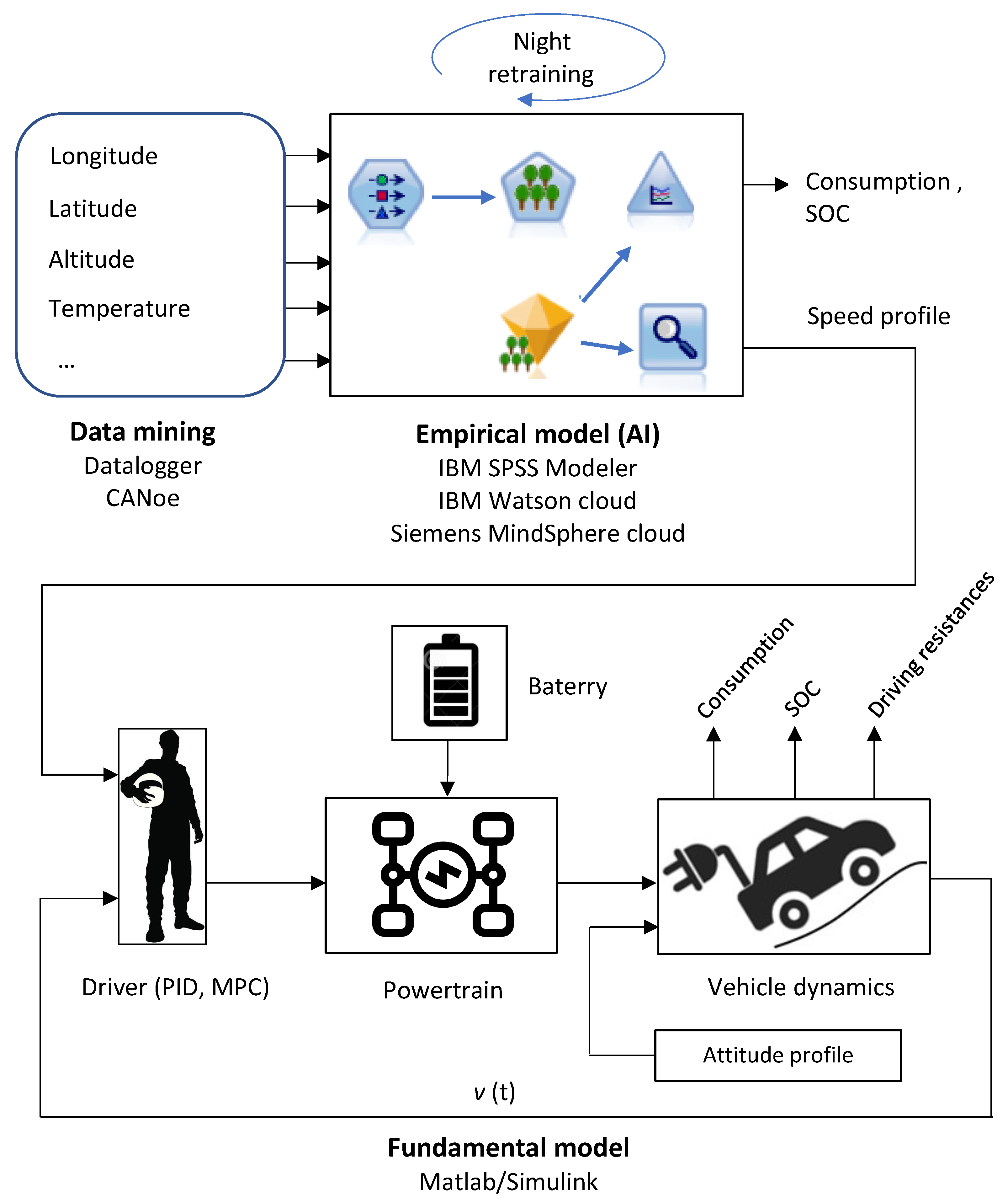
2. Biro Electric Vehicle Hybrid Research Model

As stated in the Introduction, the energy model of the Estrima Biro electric vehicle was chosen to provide the possibility of linking the empirical and fundamental model of the longitudinal dynamics. The uniqueness of the research lies in electric vehicle models created for a specific vehicle using cost-optimal parameterizations, as well as the implementation of a cloud solution that is based on own data communication, own data mining and cost-optimized parameterization of off-cloud machine learning algorithms using IBM SPSS modeler or Google Colab. The connection between the two models and the creation of the hybrid model is made possible via the speed profile, where the test cycle is extended by the altitude profile of the route. The hybrid model is shown (Figure 1). The details of this research platform will be described below.

2.1. Data Mining

A custom Datalogger has been developed and integrated to the experimental vehicle for real-time driving data measuring, see (Figure 2). The Datalogger is connected to both CAN buses of the Biro electric vehicle and, in addition to recording signals, it sends selected GNSS signals to CAN Comfort every 1000 ms. In addition to this data collection approach, we conducted our own research into cloud services using IoT operating systems with data processing applications on the IBM Watson and Siemens MindSphere platforms. In principle, it is possible to send data to the cloud or your own server in two ways. The first way is to store data in the ESP32 RAM buffer and send it online at certain intervals. This method requires active WIFI or GPRS/LTE. A WIFI platform is native with ESP32, however, the WIFI network is not always available, so the data logger is equipped with a GPRS module with a SIM card. Most IoT cloud services are designed specifically for such data transmission. However, the data series coming to the cloud in this way will be allocated to cloud time. On the WIFI network in the test environment, a stress test was performed in the IBM Watson cloud and the differences in times are up to several hundred ms. In the case of GPRS/LTE, the number is even higher. There is also a risk that data will not reach the cloud at all. To eliminate, or at least alleviate these shortcomings, it is more advantageous to use the second method, which records the entire journey on the SD card and sends all data to the cloud when the vehicle arrives back at share point. In case of failure, the data is still on the SD card. Therefore, the cloud service should support working with time information from the vehicle or RTC. If it is necessary to record data when the vehicle is parked, typically when charging, it is possible to extend the interval between recordings to several minutes or hours.

2.2. Empirical Model

In practice, it is not easy to predict which machine learning algorithm will be the best to solve a particular problem [18]. However, there is a general approach that focuses on key issues and shortlisting decisions. In the first step, we first need to get the data we want to analyze. In our case, it is telemetry data from each ride of the Biro electric vehicle coming from the Datalogger or from the cloud, if it is sent there by the Datalogger. The data can be stored in a text file, csv file, JSON format, etc. The data must be converted to meaningful values describing the investigated quantities (such as speed, temperature, latitude) and then must be modified (e.g., if stored in coded format or in case of outliers or when data is completely missing). All this happens in the second step of data preprocessing. In the third step, the inputs (features) are selected so that they best describe the outputs (labels). Feature engineering is one of the key steps in creating machine learning models. In the fourth step, the data is usually divided into training and test data. The ratios may vary depending on the application, however, as a rule, 80% of the training data and 20% of the test data can be used. The fifth step is followed by the first training and testing of the selected model. In the sixth and final step, the validated model is deployed in the final application, which can be an embedded system, cloud or mobile application.

IBM’s SPSS modeler environment version 18.2.1 is chosen for research and modeling in machine learning [19]. This tool is very efficient and, above all, provides a fast off-line analysis of input data, creating testing and validation of predictive models based on state-of-the-art machine learning algorithms. This tool was chosen based on a comparison of the speed and difficulty with which like results can be achieved, e.g., a linear regression of the prediction of students’ final scores based on individual year results. The dataset is available from the UCI Machine Learning Repository [20]. The comparison was made between a very popular open-source approach using Python, the scikit-learn machine learning library under Google Colab and SPSS modeler. The open-source approach has the advantage of flexibility and is native to running in a cloud environment, but the tax on flexibility is three to five times lead time required to get acquainted with all supporting libraries for data manipulation and visualization such as NumPy, Pandas, Anaconda, Matplotlib, etc. Moreover, extra time is required for manually entering the application code. On the other hand, a commercial SPSS Modeler, e.g., Simulink, provides pre-programmed blocks that interconnect very intuitively and fully graphically. It is also possible to transfer models created off-line to a PC, and then to the IBM Watson cloud, which is also an important parameter when choosing a research platform. For the purpose of predicting the speed profile, consumption and classification of the driver’s driving style using machine learning, a test route is selected (Figure 3). The route begins and ends at FEI’s (Faculty of Electrotechnics and Informatics) laboratory garage, where traffic conditions are ideal for simulating real situations and influencing the speed profile. The area speed limit is 30 km/h, there are three intersections with traffic lights, a variable road slope with a total value of 19 m, one speed bump and nine pedestrian crossings. Telemetry data is obtained using the developed Datalogger [21].

In addition to telemetry data, for the purposes of driver classification or driving style, data is also created as drivers enter it into a mobile application when renting a Biro vehicle (http://esharing.vsb.cz, accessed on 4 July 2020). Responses are sent to the access control unit integrated in Biro and connected to the CAN_Comfort bus. Here, the data is available under ID 0x44 with a message length of 5 bytes and refreshed in cycles every 1000 ms. The initial analysis scheme, modelling of the speed profile and consumption prediction for the test route is implemented in a classroom setting in order to select the most suitable algorithm. Vehicle speed and consumption on a given route are the predictive values. Both of these values are recorded by the Datalogger while driving and represent the machine learning input. Three best XGBoost Tree algorithms, KNN and CHAID, will be investigated.

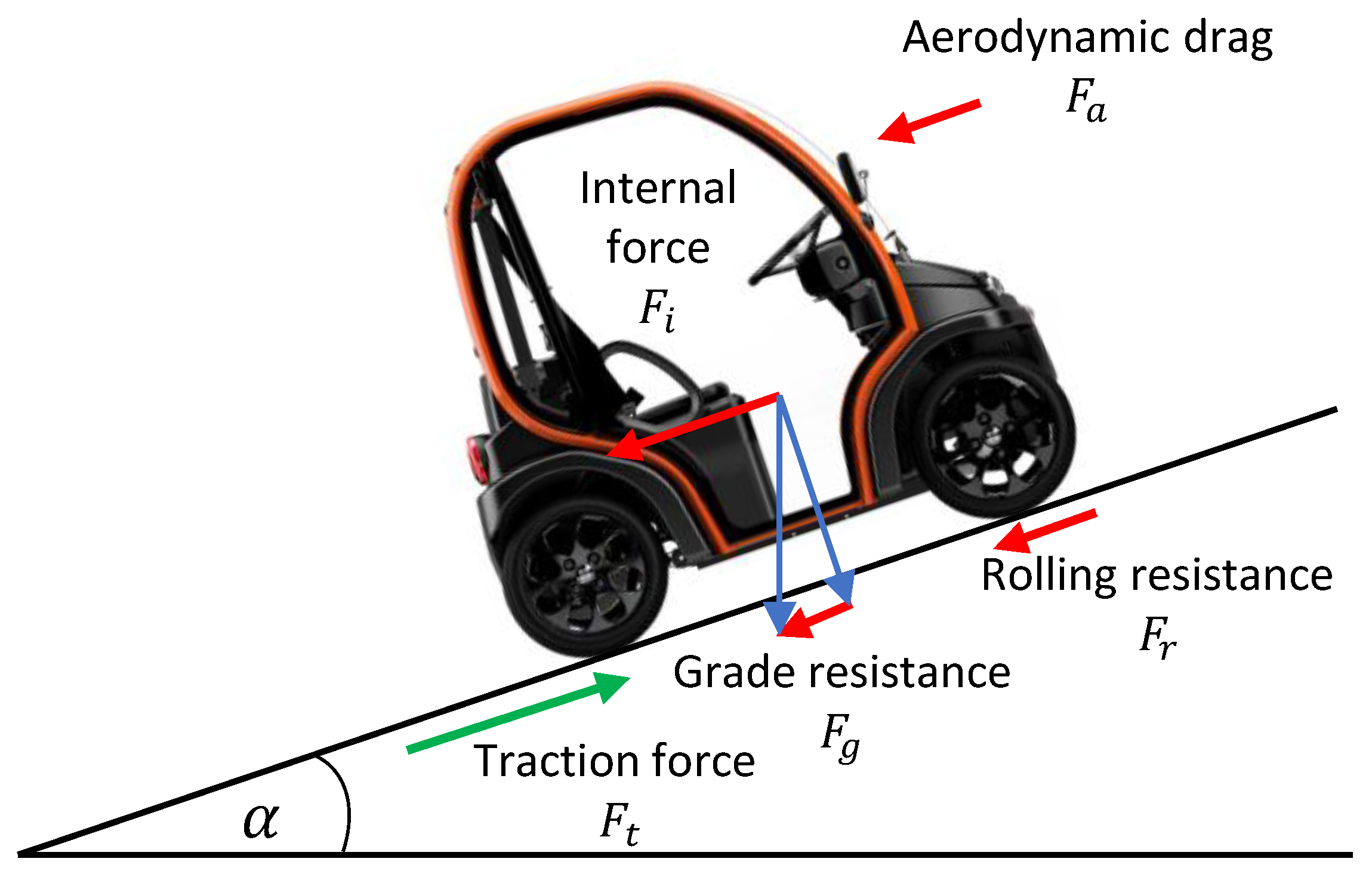
2.3. Fundamental Model

For the fundamental modelling, the speed profile and the elevation profile of the route are the input variables from which driving resistance and total consumption are calculated. In addition to the above, the fundamental model must take into account the energy flows required to overcome the driving resistances and the energy required to power the on-board network. Therefore, two models meeting these conditions are chosen as the basis for the research [22,23]. The driver plays the role of the controller and the regulated system is thus the vehicle itself, described by the longitudinal dynamics of the vehicle, which is represented by driving resistances.

The first model (Figure 4) is lossless; allowing monitoring of only basic mechanical quantities such as acceleration, speed, distance travelled, individual driving resistances and their corresponding power, energy during driving using WLTC or real driving speed, and altitude profiles of the route. This model is particularly advantageous for initial tuning of the controller (virtual driver) and studying the effect of individual driving resistance components for a particular vehicle model, e.g., at different speeds, accelerations, crew weights and gradients. This model also allows the maximum possible recuperation to be monitored. On the other hand, the disadvantage of this model is the inability to monitor or set the electrical quantities of individual components such as the battery, engine and comfort features. In order to track the electrical quantities of these components, blocks representing the losses of these components need to be added. Thus, the model (Figure 5) is based on the approach of modeling components by their losses. This approach has several advantages, such as relative simplicity, clear description in literature and adaptability to components with motor-generator operation. These are quadratic equations whose coefficients can be determined by measuring or parameterizing the model. For the lossless model, it completely adopts the basic blocks Driving Cycle, Driver and Driving Resistances of the basic lossless driving resistance model of (Figure 4). The model has been adapted for the Biro electric vehicle, which does not have a gearbox.

The driving cycle block represents the normalized form of the vehicle speed over time. Individual cycles vary in duration, distance travelled, time and percentage of stops, maximum speed, average speed with and without stops and maximum and minimum acceleration. In the case of our research platform, the data is collected using Datalogger. Two types of controllers are used in the Driver block. The PID controller is typical of the closed loop simulation structure. In such simulations, a feedback loop is introduced to calculate the deviation of the desired and calculated quantities. This deviation determines the magnitude of the control intervention. In the case of a lossless-based model (Figure 4), the desired/target quantity is the vehicle speed $v_c$ given by the driving cycle and the calculated quantity is the vehicle speed v calculated in the driving resistance block. Based on this deviation, the requirement for the tractive force $F_t$, which is the output of the driver block, is determined. In the case of the loss-based model (Figure 5). The quantities are different because there are component loss models between the driver block and the driving resistance block. In this case, the output of the driver block is the accelerator pedal position $A_p$, which is the input to the engine block, and the brake pedal position $B_p$, which is the input to the brake block. The PID controller is used for its simplicity, especially for the initial debugging of the whole model. However, for the research platform, a more sophisticated controller is used according to [24] with nonlinear dynamic optimization and control capability with a wide range of settings and support in the form of an APM library. Such dynamic control is called MPC (Model Predictive Control) and can be thought of as an optimization numerical problem where we minimize the difference between the measured output of the real system (in our case described by the nonlinear differential Equation (2) of the driving resistances) and the reference or target value. Thus, it is the minimization of the difference between the speed of the Biro electric vehicle which is the so-called reference trajectory and the simulated output of the dynamic model of the driving resistances, the controlled variable CV. We manipulate the accelerator pedal which represents the manipulated variable MV. For each step in a short time horizon, an optimization problem is run that predicts the output of the system based on the change in the input. This method of control is very flexible, but the flexibility is traded off for a higher computational complexity.

The Vehicle Dynamics block is implemented as a vehicle model on an inclined plane representing its driving resistances [25,26,27]. The assumption is that the tractive force must overcome all the driving resistances. The driving resistance is defined as the force acting against the motion of the vehicle. In addition to the driving resistances in (Figure 6), cornering resistance is also found in [26]. This resistance will be neglected because it cannot be verified in laboratory conditions at the university.

The total driving resistance or tractive force $F_t$ is given by the sum of the partial driving resistances of the vehicle

$$F_t=F_a+F_i+F_g+F_r\left(\mathrm{N}\right)$$

(1)

In the block of driving resistances (Figure 4 and Figure 5), Equation (2) is implemented in the Simulink environment, which is obtained by deriving the vehicle acceleration a, from the acceleration resistance, and substituting it into Equation (1). The resulting velocity v from the block of driving resistances, which is the input for the driver block deviation, is then obtained by integrating the acceleration a. The distance travelled is obtained by integrating the velocity v. If the individual driving resistance losses need to be investigated, the given driving resistance needs to be multiplied by the velocity. The energy can be obtained by integrating the power/losses.

$$a=\frac{F_i}{J·m}=\frac{F_t-(F_a+F_r+F_g)}{J·m}\left(\mathrm{m}·{\mathrm{s}}^{-2}\right)$$

(2)

The internal resistance $F_i$ represents the force required to change the acceleration of rotating parts such as the engine, transmission and wheels and to change the acceleration of the vehicle, which has the mass m. The influence of the rotating parts depends on the moments of inertia K, the radius of the wheels r, their number n, and the gear ratios i. In practice, the measurement of the moments of inertia of the individual rotating parts is difficult, therefore their influence is replaced by the coefficient of influence of the rotating parts J. Rotating parts of the vehicle can increase the force required by about 7% [25].

The grade resistance $F_g$ is given by Equation (3). The vehicle mass m and the angle of climb or descent of the road $\alpha$ are significant in this relation. During ascent, the drag acts against the tractive force and during descent, it contributes to the tractive force. Different approaches are used in this paper to determine the angle of climb. Namely by converting the magnitude of pressure from barometric sensor to altitude, GNSS elevation data and the DMR digital elevation model. Details of the measurements and results are given in the Results of experiments section.

$$F_g=m·g·sin\left(\alpha \right)\left(\mathrm{N}\right)$$

(3)

The rolling resistance $F_r$ is given by Equation (4) and the significant factors in this relation are the vehicle mass m, the rolling resistance coefficient $C_r$ (which depends on the road surface) the wheel inflation and the vehicle speed. For simplicity, values of 0.01–0.02 are given in practice for asphalt [25]. As the angle $\alpha$ increases, the rolling resistance decreases. In other words, the rolling resistance on a horizontal road is the highest.

$$F_r=m·g·C_r·cos\left(\alpha \right)\left(\mathrm{N}\right)$$

(4)

The aerodynamic drag $F_a$ is given by Equation (5). The most important role here is played by the square of the sum of the vehicle velocity v and the side wind velocity $v_p$. The side wind velocity increases in importance at low speeds, but since it is difficult to measure and is a practically unpredictable characteristic, it can only be considered for theoretical simulation of the impact assessment. The velocity of the side wind $v_p$ depends on the angle $\beta$ at which the side wind blows, where 90${}^{\circ }$ is the side wind in the vehicle axis. If it blows towards the front of the vehicle, the resulting air speed increases. If it blows towards the rear of the vehicle the resulting air speed decreases.

$$F_a=\frac{1}{2}·\rho ·C_a·A{(v\pm v_{p}cos\left(\beta \right))}^2\left(\mathrm{N}\right)$$

(5)

The specific air density $\rho$ depends on air temperature and pressure. The determination of the rolling resistance coefficient $C_r$ and the aerodynamic drag coefficient $C_a$ (by means of a coast down test), is described in detail for the case of the Biro electric vehicle in the Results of experiments chapter.

At the input of the engine model, the accelerator pedal position $A_p$ is multiplied by the gain given by the maximum engine torque $M_{mm}$ from which the recovery torque of the brake block is subtracted. Recuperation activates at $\mathrm{SOC}<85$%. Dividing the engine torque by the wheel radius r gives the tractive force to which the friction braking force of the brake block must be added. The resulting tractive force is the input to the vehicle dynamics block. Multiplying the motor torque by the angular velocity of the motor gives the motor power. The motor loss block implements the motor and inverter loss values from the measurements detailed in the Results of experiments section.

The brake model determines the magnitude of the frictional braking force $F_f$ for the engine block based on the accelerator pedal position input signal $B_p$. The model has as a parameter the maximum braking force $F_{bm}$, which is used to define the brake pedal position gain.

A battery model with internal resistance is used to model the battery. This model is independent of the battery chemistry. In this model, the sum of the motor input power P, and the active power of Biro’s given electrical equipment are used to calculate battery power. The objective is mainly to calculate the battery current as a basic quantity from which the SOC, battery capacity, battery power dissipation, and terminal voltage under battery load are determined. The basic relations to describe the battery are the total battery power $P_b$ as the difference of the ideal power $P_{id}$ and the power dissipation $P_{zb}$ according to Equation (6).

$$P_b=P_{id}-P_{zb}=I·V_O-I^2·R_i\left(\mathrm{W}\right)$$

(6)

The value of the battery’s open load terminal voltage $V_O$ can be measured very easily, and the value of the battery’s internal resistance $R_i$ can be measured directly using a dedicated instrument. And the state of the battery charge which is given by:

$$\mathrm{SOC}\left(t\right)=\mathrm{SOC}\left(0\right)-\frac{100}{(E_b·3600·1000)}{\int }_1^T{P}_{id}\left(t\right)\mathrm{d}t(\%)$$

(7)

3. Results of Experiments

All experiments are verified on the Estrima Biro electric vehicle, which forms the university’s carsharing platform. In its basic version, it reaches a top speed of 45 km/h and total power of 4 kW. The Biro is powered by two brushless 3f motors (BLDC) type H 130–35 from H.T.M. srl with a nominal voltage of 48 V and an output of 2 kW at 600 rpm, located directly in the rear wheels. There are, therefore, no other rotating parts such as axles, gearbox and etc. Recuperation is active at $\mathrm{SOC}<85$%. The inverters are equipped with a 250 kbit/s automotive CAN bus and operate with a nominal DC voltage of 48 V. There are many signals on this bus, internally named CAN_Motor. To protect sensitive data, no identifiers or other details of CAN messages or their signals are given in this article. Biro has one central control unit which has several functions. The CAN_Motor bus is connected to it and some of the signals from this bus are forwarded to its own bus named CAN_Comfort, which again has a baud rate of 250 kbit/s. The central control unit then communicates with the multifunction speed display via this bus and shows some driving data such as SOC and error codes in the event of an error on its LCD. It also sends the statuses of all the dashboard controls it monitors to this bus. Two types of lithium traction batteries are available for the university Biros. The first type, under the trade name Lithium Maxi, is fixed and provides a range of approx. 100 km. It is integrated in a robust and solid plastic casing. It has a nominal voltage of 44.4 V and a capacity of 111 Ah. This battery is composed of 12 LiPo (Lithium Polymer) pouch cells, which corresponds to a nominal voltage per cell of 3.7 V. The operating voltage range of a LiPo cell is normally from 3.0 V when discharged to 4.2 V when fully charged. The voltage of the entire traction battery pack therefore varies from 36 V to 50.4 V. The other available traction battery has a nominal voltage of 51.8 V and a capacity of 100 Ah.

3.1. Elevation Profile of the Route

As mentioned in the previous chapter, the input signal to the vehicle dynamics model is the road slope angle $\alpha$ in addition to the vehicle speed v. Four methods for determining elevation profiles (or slope angle) are described below.

3.1.1. Route Elevation Profile Determined from BME280 Barometric Pressure Sensor Data

The BME280 combines barometric pressure, humidity and temperature sensors in one casing. The pressure sensor itself is an absolute barometric pressure sensor and provides very high accuracy and resolution while maintaining low noise. The operating range is 300 to 1100 hPa, the RMS noise is 0.2 Pa, equivalent to 1.7 cm in height. The error is $\pm 0.25$%, equivalent to 1 m per 400 m of height change and the temperature coefficient is $\pm 1.5$ Pa/K, equivalent to $\pm 12.6$ cm per 1 ${}^{°}$C of temperature change. The digital interface of the sensor is either I2C or SPI bus. The sensor provides a native barometric pressure reading, however, this can easily be converted to an altitude at a given location. When determining road slope $\alpha$ the change in elevation of the route needs to be monitored; not its absolute value. Therefore, the otherwise required height calibration of the sensor according to a known height point at the measurement location is not necessary.

3.1.2. Route Elevation Profile Determined from GNSS Receiver uBlox Neo-M8N

The determination of the altitude profile of a route is decided by the GNSS is innacurate. However, a sensor must be used to record longitude and latitude data used in determining vehicle movement. This is necessary to generate the height profile from the DMR and for comparison with other methods. An important factor in determining the quality of the GNSS reception is the pDOP, which is determined by the geometric arrangement of the receiving satellites and, in simplified terms, the narrower the angle of view between the satellites from the receiver’s perspective, the worse the pDOP (Dilution of precision). For practical measurements, a pDOP value of 4 or less indicates a suitable arrangement and guarantees accurate positioning. With a pDOP value in the range of 5 to 7, the arrangement is still acceptable, while a value greater than 7 indicates a poor arrangement [28]. From the performed test, the visualization of the elevation profile of the route in the Matlab environment can be seen on the left (Figure 7). Matlab also provides an easy visualization of recorded longitude and latitude using the webmap function, which uses the unpaid OpenStreetMap services with a web interface. The red curve in the picture is the drive from the FEI university parking lot, where the Biro garages are located, to the U-turn point. The blue curve is then the ride from the U-turn point back to the university. The route with the turning point was deliberately chosen to study the symmetry of the measured data. In other words, the elevation profile of the blue and red routes should ideally be the same. Once a Biro is in the garage with a very weak GNSS signal, a randomly changing blue curve can be seen.

3.1.3. Route Elevation Profile Determined from a Czech Republic Digital Relief Model

The previous two methods for determining the elevation profile of a route used physical sensor data directly. The method described in the following uses GNSS route data as input to a publicly available digital elevation model, generally referred to as a DEM. The DMR is, therefore, specific to the Czech Republic. It is created and updated by digital stereophotogrammetry methods and, in selected areas, by airborne laser scanning. User interaction with the model is possible in a non-paid version via web interface [29]. It is this interface that is used to generate the elevation profile of the route from their coordinates obtained from the Datalogger. Longitude and latitude data are stored in the Datalogger in as text. For DMR, however, the data needs to be converted to GPX or SHP format. For this purpose, the available, free web application www.gpsvisualiser.com, can be used. When generating the GPX file, it is important to enable track type attributes (since routes, route points, and waypoints are not supported by DMR) and to follow the principle of (Figure 8).

A visualization of the same route as in OpenStreetMap is shown in the DMR web interface, screenshot on the right (Figure 7), where a shaded relief (Z-factor 10) with zero transparency is used. The final step is to generate the actual elevation profile of the route. This is possible after loading the route in SHP format onto the web interface. In this step, it is necessary to select the route segmentation for calculating the height, either in meters or in data points, i.e., points recorded by the Datalogger. The second option is preferable since, in Matlab, the number of points in the altitude profile is then consistent with the number of points on the route and there is no need to use linear regression to resample points in the graphs, which always require the same number of points on both axes.

3.1.4. Route Elevation Profile Determined from the Mapy.cz Planner

A Czech route planner, Mapy.cz, is a part of the www.seznam.cz portal. It is updated once a week for the Czech and Slovak Republics and these map documents are created directly by Mapy.cz. Foreign map documents are updated once a month. The maps of European countries have been adopted from Navteq since 2011 and since 2014 they have been adopted from the OpenStreetMap opensource project [30]. Similar to DMR, it is possible to import driving data in GPX format onto the web interface and the same constraints apply to, i.e., the track type attribute. Mapy.cz displays the elevation profile of the driving route directly on the web interface. The export of the elevation profile is possible either in GPX or KML format. For Matlab, the GPX format is preferred because it can be easily processed using the gpxread function. The elevation profile of the route is calculated from a digital model created by different sources.

3.1.5. Comparison of the Results of Height Profile Measurements Using the above Methods

Figure 9 shows a comparison of the altitude profiles obtained by the four different methods described above. All the profiles should be symmetrical around 1220 m, where the turn and return to the exit point-the university garage-was created. The elevation data obtained from the GNSS receiver is highly inaccurate compared to the data from the other three methods, although the pDOP ranged from 2.1 to 4.2 up to 2400 m. The GNSS method for measuring the elevation profile of the route will not be further developed as it does not have sufficient accuracy for civil or non-commercial use. However, the recording of longitude and latitude coordinates still remains an integral input for DMR. The other three methods are significantly better in accuracy and one can see not only symmetry around the turning point, but also a consistent route profile. The elevation profile obtained from the barometric sensor has an offset of 3 m, but this is due to the non-calibrated BME280 sensor for absolute altitude. As already mentioned, the absolute altitude is not essential because the objective is to determine the slope of the route for the vehicle drag model, which is determined relatively from the differences in altitude at selected segments along the route.

3.2. Determining Aerodynamic and Rolling Resistance Coefficients

In practice, the coefficient of air resistance $C_a$ and the coefficient of rolling resistance of wheels $C_r$ are most often measured using four methods [31]. The wind tunnel test, where the vehicle or its dimensional ratio model is stationary and surrounded by a controlled amount of air. The drag force of the air onto the vehicle is measured. This method, therefore, only allows the air drag coefficient to be determined. The advantage lies in the possibility of testing different angles of air flow as well as different air velocities. CFD analysis, which uses a numerical simulation of a virtual vehicle model being subjected to an air stream to determine the air drag coefficient. Like the wind tunnel test, it is possible to simulate different angles of the airflow as well as its different velocities. The constant speed test, (no longer a laboratory test), is a test where the vehicle speed is kept constant for two or more selected speeds. Torque, wind direction and speed are measured. It is the measurement of torque that requires the use of special and expensive equipment. This test is the only test accepted for certification procedures in the European Union. The coast down test is not a laboratory test, either. The vehicle, after reaching a certain speed, disengages from the drive after disengaging and depressing the clutch and is allowed to slow down naturally with a constant measurement of the vehicle speed over time; in our case using the Datalogger described above. A complete stop of the vehicle is not a prerequisite for ending the test. For this test, the slope of the route, the wind direction, and the speed must be taken into account. The influence of these two factors on the measurement results can be considered a disadvantage of this method, but the overriding advantage of simplicity largely eliminates this fact. This test is the primary method in the Greenhouse Gasses standard (GHG) measurement procedure defined by the U.S. Environmental Protection Agency (US EPA). The result of the test is a range characteristic that describes the dependence of the measured driving resistance on vehicle speed. In the case of Biro, taking into account complexity, cost and lead time, the coast down test is chosen. It takes advantage of the fact that the tractive force $F_t$ is zero. Equation (1) is thus reduced to the form:

$$0=F_a+F_i+F_g+F_r\left(\mathrm{N}\right)$$

(8)

After adding from Equations (3)–(5) we can express the acceleration or deceleration as:

$$\begin{array}{c}\dot{v}·Jm=-F_a-F_g-F_r=-\frac{1}{2}·\rho ·C_a·A·{(v\pm v_p·cos\left(\beta \right))}^2+\\ -g·sin\left(\alpha \right)-g·C_r·cos\left(\alpha \right)(\mathrm{m}·{\mathrm{s}}^{-2})\end{array}$$

(9)

Measurements are to be made on a roadway having a longitudinal slope of up to $\pm 1$% and wind speeds of 1.5 m·s${}^{-1}$. The air temperature on the day of measurement was 2.1 ${}^{°}$C. In the case of the Biro measurements, the test route has an elevation of 2 m over a 127 m length, as can be seen (Figure 10). The start position (GPS 49.8388478N, 18.1391908E) is fixed, indicating with a traffic cone the point at which the vehicle started to decelerate or the driver fully released the acceleration pedal. The stop position is illustrative and depends on the speed of the vehicle when passing through the start position. The wind speed was only measured statically before each test ride, not continuously with an anemometer. The wind speed on the day of the measurement was no higher than 1.3 m·s${}^{-1}$. Therefore, Equation (9) reduces to:

$$\dot{v}·Jm=-F_a-F_g-F_r=-\frac{1}{2}·\rho ·C_a·A_v^2-g·sin\left(\alpha \right)-g·C_r·cos\left(\alpha \right)(\mathrm{m}·{\mathrm{s}}^{-2})$$

(10)

From Equation (10), we determine the aerodynamic and rolling resistance coefficients using dynamic estimation. The determination of the parameters has a similar mathematical basis as the MPC. Using a numerical method to minimize the difference between the measured output of the real system (in this case the Biro vehicle) and the simulated output of the dynamic model given by the differential Equation (10) of this system, we determine both coefficients. The objective function and the conditions are of the Equation (11).

$$\begin{array}{c}\underset{C_a,C_r}{min}{\Vert v_m-v\Vert }_n\\ \mathrm{s}.\mathrm{t}.\dot{v}·Jm=-\frac{1}{2}·\rho ·C_a·A{v}^2-g·sin\left(\alpha \right)-g·C_r·cos\left(\alpha \right)\\ 0\le C_a\le 1\\ 0\le C_r\le 1\end{array}$$

(11)

Thus, we find both coefficients by minimizing the measured velocity $v_m$ and the simulated velocity v under conditions that constrain both coefficients to positive values less than one. In (Figure 11), we can see the vehicle velocity measurement from the start point to the stopping point. The numerical solution is performed using Matlab in conjunction with a free, APM optimization library [24,32].

In the case of the Biro, coast down tests were carried out at three different tyre pressures to determine the effect on the rolling resistance coefficient. The simulation results are shown in

Table 1. Aerodynamic and rolling resistance coefficients of the Biro electric car.

Tire Pressure (kPa)	Sample Time (ms)	Simulation Time (s)	${\mathit{C}}_{\mathit{a}}$ (−)	${\mathit{C}}_{\mathit{r}}$ (−)
300	20	45.657	0.482	0.032
300	200	0.409	0.460	0.032
260	20	41.786	0.442	0.033
260	200	0.389	0.471	0.033
200	20	38.697	0.437	0.035
200	200	0.378	0.423	0.035

. As expected, the rolling resistance coefficient increases with decreasing tyre pressure. The aerodynamic drag coefficient shows variations due to the effect of wind speed, which is a factor at low vehicle speeds and was not measured continuously. The aerodynamic drag alone, and its non-significant importance, would not justify the cost and complexity of continuously measuring wind speed during the range test. The table also shows the simulation computation time for any real-time computation needs directly in the vehicle with different sampling of the speed signals with the CAN bus. The computation time is for a quad core Intel Core i7-8550U @1.8 GHz processor. As we can see the difference in speed sampling is tenfold. However, the difference in computation times is more than a hundredfold.

3.3. Verification of Driver Block Functionality

The driver block contains a PID controller. The controller parameters do not need to be changed for different drive cycles. This is thanks to the fact that the regulated system, i.e., the Biro, has fixed constants entering the modelling of the tractive force. Respectively, individual driving resistances (i.e., the aerodynamic and rolling resistance coefficient), the coefficient of influence of rotating parts, the size of the frontal area of the vehicle, the air resistance coefficient, and changing variables such as the weight varying within the range given by the weight of the driver and passenger, the limited range of climb and descent angles given by the road design and the relatively low power of the electric motors. All these basically determine the acceleration dynamics of the vehicle, in other words the change in vehicle speed over time, which for such a small vehicle does not have a wide range and the fixed PID is able to regulate very well for different driving cycles. The difference between the measured speed and the simulated speed can be seen (Figure 12).

The model comparing the PID and MPC controller is shown (Figure 13). MPC is implemented using a Matlab function with three input parameters. The first parameter of the function is the desired target speed, the second parameter is the speed from the Biro drag model, and the third parameter is the slope angle of the route. The output of the function is the traction force, which is the input to the Biro drag model. The required speed and path slope angle are available in the VSB_MSIC structure and contains the same driving data as in (Figure 7). The actual comparison between the PID and MPC controller is shown (Figure 14) for the three essential variables of traction power; traction, energy and speed. The traction power waveform of the PID controller (red curve) shows seemingly more instability compared to the MPC waveform (blue curve), due to the higher speed of the PID controller.

The MPC regulation speed is slower for all waveforms, due to the higher computational time requirements, and reaches up to 800 ms according to the simulation. This delay consists in a minor part due to the actual solution of the numerical optimization problem in APM and, in a major part, due to the Matlab/Simulink environment itself, which uses an interpreted function that must first be translated by the Matlab parser during each run. The average computational speed of the optimization problem in APM is 21.6 ms for the 5 s horizon, 32.8 ms for the 10 s horizon, and 56.8 ms for the 15 s horizon. The traction energy waveform above (Figure 14) is very similar for both controllers. The MPC (blue curve), due to its lower regulation speed, naturally filters the traction power changes and thus helps to reduce the power consumption, however, the main advantage of the MPC is the ability to design the objective function of the optimization problem. The actual speed of the Biro is shown in yellow in the velocity or speed profile, bottom of (Figure 14). The controller has the task of tracking this target speed as accurately as possible. The PID controller (the red curve merges with the yellow at a given resolution) succeeds very well. The MPC controller’s velocity waveform (blue curve) does not copy the target velocity as well as PID, but the controller has other, more significant, advantages.

The MPC regulation speed is slower for all waveforms due to higher computational time requirements and reaches up to 800 ms according to the simulation. This delay is partly due to the actual solution of the numerical optimization problem in APM. However, it is mostly due to the Matlab/Simulink environment itself, which uses an interpreted function that must first be translated by the Matlab parser during each run. The average computational speed of the optimization problem in APM is 21.6 ms for the 5 s horizon, 32.8 ms for the 10 s horizon, and 56.8 ms for the 15 s horizon. The traction energy waveform in Figure 14 above is very similar for both controllers. The MPC (blue curve), due to its lower regulation speed, naturally filters the traction power changes and thus helps to reduce the power consumption. However, the main advantage of the MPC is the ability to design the objective function of the optimization problem. The actual speed of the Biro is shown in yellow in the velocity or speed profile, bottom (Figure 14). The controller has the task of tracking this target speed as accurately as possible. The PID controller (the red curve merges with the yellow at a given resolution) succeeds very well. The MPC controller’s velocity waveform (blue curve) does not copy the target velocity as well as PID, but the controller has other more significant advantages.

The effect of the length of the time horizon on the accuracy of vehicle speed determination is shown (Figure 15). MPC has overshoot to negative values, this effect can be eliminated by APM library parametr $v.lower$ or by saturation block in Simulink. As illustrated, a longer time horizon smoothens the velocity waveform, even with small changes in the velocity (see the 240–280 s time interval).

3.4. Comparison of Real and Simulated Consumption

Figure 16 compares the simulated and actual consumption of Biro for the route in (Figure 7). The crew consisted of a driver and a passenger totaling 160 kg in weight. In this simulation, a lossless model was used (see Figure 4). The dips in the red curve show the theoretical recuperation that occurs when slowing down or driving downhill.

To investigate the effect of individual driving resistances, it is necessary to know their contributions to the total consumption. Therefore, the consumption from (Figure 16) is further decomposed into the contributions of rolling resistance, aerodynamic resistance, grade resistance and internal resistance as shown (Figure 17). The largest influence is the rolling resistance of 88%, which depends not only on the rolling coefficient and, especially on the mass, which varies over a range determined by the mass of the driver and passenger. The energy consumed by aerodynamic drag, grade drag and acceleration/internal drag is not significant for this particular driving route case. The energy consumed by aerodynamic drag is 17% and will not vary much in real life operation due to the Biro’s relatively low top speed of 45 km/h. Side wind speed, which is generally neglected in the models, will also not make any significant difference. If we assume that the Biro is an urban electric vehicle driven in areas with little change in elevation, the contribution of grade resistance will be low (up to 10%). The recuperation of the Biro (see the drops in the green and red curves (Figure 17)) is available because it is supported by the native inverters used. However, its contribution is up for debate. Inverters supporting recuperation have a higher price and may not pay off.

3.5. Distribution of Consumption According to Driving Resistance

Figure 18 shows the effect of crew weight on the Biro’s consumption. The net weight of the Biro is 369 kg and the simulation shows the case of a driver with a weight of 80 kg and no passenger is 449 kg, whereas with a passenger of 80 kg it weighs 529 kg.

3.6. Measurement of Motor and Inverter Losses

The aim of the measurement is to determine the losses of motors and their converters for the motor model. The measurement was performed on a MAHA-LPS 3000 university laboratory dynamometer. The dynamometer was set to a mode of maintaining a constant speed, where it is possible to regulate the magnitude of the traction force F [N] displayed by the dynamometer dashboard. The power P [kW] dynamometer calculates according to relation (12). This is the net mechanical power on the dynamometer rollers and in real conditions corresponding with the mechanical power transmitted to the road. It should be noted that there are losses between the wheels and the rollers due to rolling resistance. We calculate these losses according to the formula in (13). In this relation, the weight of the vehicle is $m=449$ kg, the angle of the road $\alpha =0^{\circ }$ and the selected rolling resistance coefficient with respect to smooth cylinders $C_r=0.02$. Each wheel runs on two dynamometer cylinders. During the measurement, the battery current $I_b$ and the battery voltage $U_b$ were read from the CAN_Motor bus using the CANoe program, where these values are available. The losses on the motor and inverter are given by Equation (14). For clarity, the torque $M=Fr$ is added in table

Table 2. Motor and converter loss measurement results.

v (km/h)	F (N)	M (Nm)	P (kW)	${\mathit{U}}_{\mathit{b}}$ (V)	${\mathit{I}}_{\mathit{b}}$ (A)	${\mathit{P}}_{\mathit{e}}$ (kW)	${\mathit{P}}_{\mathit{v}}$ (kW)	${\mathit{P}}_{\mathbf{mm}}$ (kW)	${\mathit{\mu }}_{\mathbf{mm}}$ (−)
15	100	25	0.4	44.65	23	1.03	1.03	0.35	0.66
15	200	50	0.9	44.52	35	I.56	1.56	0.38	0.75
15	300	76	1.3	44.3	48	2.13	2.13	0.55	0.74
15	400	101	1.8	44.1	61	2.69	2.69	0.61	0.77
15	500	126	2.1	43.8	75	3.29	3.29	0.91	0.72
15	760	192	3.2	42.5	120	5.10	5.10	1.62	0.68
25	50	13	0.4	44.3	29	1.28	1.28	0.43	0.67
25	100	25	0.8	44.21	37	1.64	1.64	0.38	0.77
25	200	50	1.4	43.9	55	2.41	2.41	0.56	0.77
25	300	76	2.1	43.6	74	3.23	3.23	0.67	0.79
25	505	127	3.5	42.6	118	05.03	05.03	11.07	0.79
30	60	15	0.5	44	35	1.54	1.54	0.49	0.68
30	100	25	0.9	43.8	44	1.93	1.93	0.48	0.75
30	200	50	1.7	43.6	66	2.88	2.88	0.63	0.78
30	246	62	2	43.3	75	3.25	3.25	0.70	0.79
30	420	106	3.5	42.7	120	5.12	5.12	1.07	0.79
40	62	16	0.7	43.6	50	2.18	2.18	0.75	0.66
40	94	24	1	43.38	57	2.47	2.47	0.74	0.70
40	165	42	1.8	43.07	77	3.32	3.32	0.78	0.76
40	293	74	3.2	42.8	120	5.14	5.14	1.20	0.77

and the efficiency of the motor with the ${\mu }_{mm}$ converter is given by the Equation (15).

Mechanical power on dynamometer rollers

$$P=F·\frac{v}{3600}\left(\mathrm{kW}\right)$$

(12)

Rolling losses

$$P_v=F_v·v=m·g·C_r·cos\alpha ·\frac{v}{3600}\left(\mathrm{kW}\right)$$

(13)

Motor and converter losses

$$P_{mm}=U_b·I_b·0.001-(P+P_v)=P_e-P-P_v\left(\mathrm{kW}\right)$$

(14)

Motor efficiency with converter

$${\mu }_{mm}=\frac{P+P_v}{U_b·I_b}(-)$$

(15)

3.7. Evaluation Metrics of the Best Machine Learning Algorithms for Speed and Consumption Prediction in SPSS Modeler

The Auto Numeric block parameter settings are not very extensive and all seventeen regression algorithms were chosen for speed prediction, with only ten of them ending up with model generation. The measured (actual) velocity profile corresponding to the route of Figure 3 of 27.8.2020, which can be seen (Figure 19), Ride 1.

Other algorithms are significantly worse, e.g., in the sixth position there is a linear regression with LC 0.354 and RE 0.871 and it will not be further investigated. Metrics are chosen for test data, which explains the increasing ratings for the growing proportion of test data, as shown in

Table 3. Evaluation metrics of the five best algorithms for speed prediction.

	Training 80%		Training 70%		Training 50%
	Testing 20%		Testing 30%		Testing 50%
	LC	RE	LC	RE	LC	RE
KNN	0.935	0.134	0.935	0.131	0.928	0.143
XGBoost Tree	0.948	0.148	0.950	0.142	0.950	0.122
CHAID	0.906	0.179	0.884	0.223	0.844	0.290
C&R Tree	0.874	0.238	0.850	0.279	0.889	0.211
Neural Net	0.783	0.390	0.792	0.379	0.726	0.482

. It is worth noting the change in order for 50% of the training and 50% of the test data, where the XGBoost Tree algorithm is better than KNN and the C&R Tree is better than CHAID. For further research, individual models of these algorithms will be compiled, which have a significantly wider setting of parameters (hyperparameters).

We proceed analogously to predict consumption. Consumption during run 1 was used for the prediction as shown (Figure 20).

As illustrated in

Table 4. Evaluation metrics of the best algorithms for consumption prediction.

	Training 80%		Training 70%		Training 50%
	Testing 20%		Testing 30%		Testing 50%
	LC	RE	LC	RE	LC	RE
KNN	0.999	0.001	0.999	0.001	0.998	0.005
Neural Net	0.999	0.001	0.999	0.001	0.999	0.002
CHAID	0.999	0.003	0.998	0.004	0.999	0.003
Linear	0.999	0.003	0.999	0.003	0.999	0.003
Regression	0.999	0.003	0.999	0.003	0.998	0.003
XGBoost Tree	0.997	0.031	0.997	0.031	0.996	0.042

, when compared to speed prediction, the XGBoost Tree algorithm does not perform as well. The KNN, CHAID and Neural Net algorithms are chosen for further research, for which individual models will be compiled and the influence of their hyperparameters on evaluation metrics will be investigated.

3.8. Speed Prediction Using Machine Learning

Speed is one of the key components of a driver’s behavior pattern. Using IBM Watson’s machine learning service, Biro data is trained to predict speed using data from its other variables, such as current, voltage, accelerometer, etc. An experiment using IBM Watson, specifically AutoAI, triggers our data using a different algorithm to “machine”. It learned to create a predictive model. Our speed training data ranges from 0 to 45 km/h (used to train this model), which means that our model will learn different combinations to predict the speed of the test data. Since our required results are in the form of velocity, they fall directly into the multi-class classification model. This means that it has forty-six (0–45) different results instead of a binary classification. XGBoost Classifier or Extreme Gradient Boosting and Linear Regressor algorithms were used to train the model. Although our conventional linear regression method seems to give decent results, the XGB classifier provides a detailed model structure for immediate analysis (Figure 21).

The basic speed detection technique deals with one dependent (predictive) variable and n is the number of independent/correlated variables. This follows a regression formula. In our case the “predictive variable” is speed and the independent variables are current, voltage and other column/series variables in MS Excel.

In Figure 22, the XGB algorithm classifier is used to train the model. On the right, we illustrate the value of a single speed (e.g., 43 km/h) compared to another line variable that uses the same speed. On the left, data on total speed compared to other variables is illustrated. We can see that the accuracy of one speed (0.98) is greater than the overall accuracy (0.347).

In Figure 23, there are three data points (F1, Recall and Precision [33]) for each speed data input. Most importantly, accurate data was used for the analysis. The red rectangle highlights accurately predictable speeds, which are 36, 37, 43 and 45 when using this training model, since its level of accuracy is high despite a low threshold (less than 0.2). Since high-speed data is more predictable and low-speed data predictability is below-average in accuracy, the overall accuracy is reduced to 0.347, illustrated in Figure 23. It is understood that not all values from 0 to 45 km/h are considered due to an error of speed tracking (recording) method, since we record data every 2–3 seconds in which the Biro reaches a certain constant speed.

4. Conclusions

This article describes a hybrid research platform linking empirical and fundamental modeling with proven results for the Estrima Biro electric car. The car belongs to the university’s carsharing fleet and is unique due to its integration of programmable systems and data logger. However, the Estrima Biro is also speciic in size, power, drive and assistance systems. For example, the dimensions of the Bira axles do not allow it to be easily measured on available university dynamometers, which has led to the natural choice of hybrid modeling of the traction drive used.

First, the issue of empirical, fundamental and hybrid modeling of electric vehicle propulsion in the longitudinal direction is described. The fundamental model is created in the Matlab/Simulink environment and represents the modeling of the vehicle’s resistance. The model includes two driver models, a simple PID controller and a more sophisticated MPC controller, enabling the optimization of driving style and, thus, consumption. In principle, this model also makes it possible to monitor the details of the individual running resistances and the corresponding energy flows. Emphasis is placed on economy, accuracy and measurement speed when determining the driving resistance of the Biro electric car. For this reason, a combination of a road test and a numerical problem of dynamic parameter estimation is chosen. The empirical model in the IBM SPSS modeler is an artificial intelligence model created for selected machine learning algorithms with a teacher. Since the Biro electric car does not have sensors enabling interaction with the environment, such as a camera for detecting traffic lights, radar for measuring distances, or a connection to the smart city infrastructure, the goal is to predict the speed profile of the ride from past data. This speed profile is then the input for the driving resistance model and this connection creates a hybrid model. The fundamental model in Matlab/Simulink and empirical models in IBM SPSS Modeler, IBM cloud and scikit-learn are created on the basis of real driving data, which is stored by a built-in recorder. Data describing the route is stored, e.g., coordinates, altitude allowing us to determine the slope of the route and data from two private CAN buses of the Biro electric car. In addition to the theoretical part, the work includes verification of all models on a specific vehicle and a specific route. For all models, a detailed description of their functional blocks and verification, using measured and model results, is available.

This research has been carried out over 2 years, where several specializations are combined with real implementations and verified by practical experiments. The article presents the results of research using a SW platform with a new type of operating systems or data processing for cloud computing (e.g. SIEMENS MindSphere, IBM IoT) and experimental verification of a new hybrid model of electric vehicle behavior. The use of a hybrid model is a new method within the selected specific application for the area of shared electric vehicles. The hybrid model minimizes the use of sensors (lidar, radar, V2x) and thus optimizes cost, which is currently a basic demand for the operation of shared vehicles. The hybrid model eliminates the disadvantages of machine learning (taking into account the cyber-physical properties of the vehicle) and the disadvantages of the model of longitudinal dynamics of the vehicle. For example, it cannot take into account the influence of traffic situations and weather. The hybrid model allows the carshare user to predict consumption and range before the ride itself and further refine the prediction while driving (i.e., when the user drives a vehicle unknown to them).

References

1. Electric Vehicle Overview Database. EV Database-v4.1. Available online: https://ev-database.org (accessed on 4 July 2020).
2. De cauwer, C.; Verbeke, W.; Coosemans, T.; Faid, S.; Mierlo, J.V. A Data-Driven Method for Energy Consumption Prediction and Energy-Efficient Routing of Electric Vehicles in Real-World Conditions. Energies 2017, 10, 608. [Google Scholar] [CrossRef] [Green Version]
3. Vajedi, M.; Azad, N.L. Ecological Adaptive Cruise Controller for Plug-In Hybrid Electric Vehicles Using Nonlinear Model Predictive Control. IEEE Trans. Intell. Transp. Syst. 2016, 17, 113–122. [Google Scholar] [CrossRef]
4. Zhang, Y.; Chu, L.; Fu, Z.; Xu, N.; Guo, C.; Zhang, X.; Chen, Z.; Wang, P. Optimal energy management strategy for parallel plug-in hybrid electric vehicle based on driving behavior analysis and real time traffic information prediction. Mechatronics 2017, 46, 177–192. [Google Scholar] [CrossRef]
5. Gilman, E.; Keskinarkaus, A.; Tamminen, S.; Pirttikangas, S.; Röning, J.; Riekki, J. Personalised assistance for fuel-efficient driving. Transp. Res. Part C: Emerg. Technol. 2015, 58, 681–705. [Google Scholar] [CrossRef] [Green Version]
6. Magaña, V.C.; Organero, M.M. Artemisa: Using an Android device as an Eco-Driving assistant. J. Sel. Areas Mechatron. (JMTC) 2011, 1–8. [Google Scholar]
7. Magana, V.C.; Muñoz-Organero, M. Artemisa: An eco-driving assistant for Android Os. In Proceedings of the 2011 IEEE International Conference on Consumer Electronics-Berlin (ICCE-Berlin), Berlin, Germany, 6–8 September 2011; pp. 211–215. [Google Scholar]
8. Magana, V.C.; Organero, M.M. Artemisa: A Personal Driving Assistant for Fuel Saving. IEEE Trans. Mob. Comput. 2016, 15, 2437–2451. [Google Scholar] [CrossRef] [Green Version]
9. Kural, E.; Jones, S.; Parrilla, A.F.; Grauers, A. Traffic light assistant system for optimized energy consumption in an electric vehicle. In Proceedings of the 2014 IEEE International Conference on Connected Vehicles and Expo (ICCVE), Vienna, Austria, 3–7 November 2014; pp. 604–611. [Google Scholar]
10. Sun, C.; Sun, F.; He, H. Investigating adaptive-ECMS with velocity forecast ability for hybrid electric vehicles. Appl. Energy 2017, 185, 1644–1653. [Google Scholar] [CrossRef]
11. Sun, C.; He, H.; Sun, F. The Role of Velocity Forecasting in Adaptive-ECMS for Hybrid Electric Vehicles. Energy Procedia 2015, 75, 1907–1912. [Google Scholar] [CrossRef] [Green Version]
12. Guo, J.; He, H.; Peng, J.; Zhou, N. A novel MPC-based adaptive energy management strategy in plug-in hybrid electric vehicles. Energy 2019, 175, 378–392. [Google Scholar]
13. Trommer, S.; Holtl, A. Perceived usefulness of eco-driving assistance systems in Europe. IET Intell. Transp. Syst. 2012, 6, 145–152. [Google Scholar] [CrossRef]
14. Magana, V.C.; Munoz-Organero, M. GAFU: Using a Gamification Tool to Save Fuel. IEEE Intell. Transp. Syst. Mag. 2015, 7, 58–70. [Google Scholar] [CrossRef] [Green Version]
15. Jamson, S.L.; Hibberd, D.L.; Jamson, A.H. Drivers’ ability to learn eco-driving skills; effects on fuel efficient and safe driving behaviour. Transp. Res. Part C Emerg. Technol. 2015, 58, 657–668. [Google Scholar] [CrossRef]
16. Report on Updating and Status Records of Fuel Filling Stations in the Czech Republic as of 9 April 2021. MPO. 2021. Available online: https://www.mpo.cz/cz/energetika/statistika/statistika-a-evidence-cerpacich-a-dobijecich-stanic/zprava-o-aktualizaci-a-stavu-evidence-cerpacich-stanic-pohonnych-hmot-v-cr-k-9–4–2021–260737/ (accessed on 17 July 2020).
17. List of Public Charging Stations-Status as of 31 March 2021. MPO. 2021. Available online: https://www.mpo.cz/cz/energetika/statistika/statistika-a-evidence-cerpacich-a-dobijecich-stanic/seznam-verejnych-dobijecich-stanic-_-stav-k-31–3–2021–260994/ (accessed on 17 July 2020).
18. Introduction to Machine Learning, Part 1: Machine Learning Fundamentals. MathWorks. 2020. Available online: https://www.mathworks.com/videos/introduction-to-machine-learning-part-1-machine-learning-fundamentals-1542879625034.html (accessed on 17 July 2020).
19. IBM SPSS Modeler V18.2.1 Documentation. IBM. 2020. Available online: https://www.ibm.com/support/knowledgecenter/cs/SS3RA7_18.2.1/modeler.kc.doc/clementine/knowledge_center/product_landing.html (accessed on 17 July 2020).
20. Cortez, P.; Silva, A. Using Data Mining to Predict Secondary School Student Performance. Proceedings of 5th FUture BUsiness TEChnology Conference (FUBUTEC 2008), Porto, Portugal, 5–12 April 2008; pp. 5–7. [Google Scholar]
21. Ozana, S.; Pies, M.; Hajovsky, R.; Koziorek, J.; Horacek, O. Application of PIL Approach for Automated Transportation Center. In Computer Information Systems and Industrial Management; Springer: Heidelberg, Germany, 2014; pp. 501–513. ISBN 978-3-662-45236-3. [Google Scholar]
22. MATLAB and Simulink Racing Lounge: Vehicle Modeling. MathWorks. 2020. Available online: https://www.mathworks.com/matlabcentral/fileexchange/63823-matlab-and-simulink-racing-lounge-vehicle-modeling (accessed on 8 July 2020).
23. Zou, Y.; Li, J.; Hu, X.; Chamaillard, Y. Modeling and Control of Hybrid Propulsion System for Ground Vehicles; Beijing Institute of Technology Press: Beijing, China; Springer: Berlin, Gemany, 2018; ISBN 978-3-662-53673-5. [Google Scholar]
24. Hedengren, J.D.; Shishavan, R.A.; Powell, K.M.; Edgar, T.F. Nonlinear modeling, estimation and predictive control in APMonitor. Comput. Chem. Eng. 2014, 70, 133–148. [Google Scholar] [CrossRef] [Green Version]
25. Vlk, F. Dynamics of Motor Vehicles, 2nd ed.; Prof. Ing. Frantisek Vlk, DrSc.: Brno, Czech Republic, 2003; ISBN 80-239-0024-2. [Google Scholar]
26. Sciarretta, A.; Vahidi, A. Energy-Efficient Driving of Road Vehicles Toward Cooperative, Connected, and Automated Mobility; Springer: Cham, Switzerland, 2020; ISBN 978-3-030-24127-8. [Google Scholar]
27. Neborak, I.; Simonik, P.; Odlevak, P. Electric Vehicle Modelling and Simulation. In Proceedings of the 14th International Scientific Conference on Electric Power Engineering, Kouty nad Desnou, Czech Republic, 28–30 May 2013; pp. 693–696. [Google Scholar]
28. Rapant, P. Satellite Positioning Systems; Vysoka Skola Banska-Technicka Univerzita: Ostrava, Czech Republic, 2002; ISBN 80-248-0124-8. [Google Scholar]
29. Digital Relief Model of the Czech Republic 5th Generation (DMR 5G). CUZK. 2018. Available online: https://geoportal.cuzk.cz/(S(4rwf2xubg35yvuzr4xlj2fyx))/Default.aspx?mode=TextMeta&side=vyskopis&metadataID=CZ-CUZK-DMR5G-V&head_tab=sekce-02-gp&menu=302 (accessed on 4 July 2020).
30. Tools for Working with the Route. Seznam.cz a.s. 2020. Available online: https://napoveda.seznam.cz/cz/nastroje-pro-praci-s-trasou/ (accessed on 4 July 2020).
31. Comparison of Aerodynamic Drag Determination Procedures for HDV CO2 Certification. ICCT. 2019. Available online: https://theicct.org/sites/default/files/publications/ICCT_aero_drag_briefing_20190814.pdf (accessed on 4 July 2020).
32. APMonitor Documentation. 2020. Available online: http://apmonitor.com/wiki/ (accessed on 25 December 2020).
33. Lever, J.; Kryzwinki, M.; Altman, N. Classification evaluation. Nat. Methods 2016, 13, 603–604. [Google Scholar] [CrossRef]
Figure 1. Hybrid model of Biro EV.
Energies 15 01300 g001
Figure 2. Block diagram of the datalogger.
Energies 15 01300 g002
Figure 3. Test route.
Energies 15 01300 g003
Figure 4. Lossless model.
Energies 15 01300 g004
Figure 5. Model enhanced by component losses.
Energies 15 01300 g005
Figure 6. Driving resistances.
Energies 15 01300 g006
Figure 7. The test route visualized in OpenStreetMap (left) a DMR 5G (right).
Energies 15 01300 g007
Figure 8. GNSS data conversion scheme.
Energies 15 01300 g008
Figure 9. Comparison of route altitude profiles.
Energies 15 01300 g009
Figure 10. Measured section of the coast down test route (a) and its elevation (b).
Energies 15 01300 g010
Figure 11. Biro Speed during the coast down test.
Energies 15 01300 g011
Figure 12. Comparison of measured and simulated speed.
Energies 15 01300 g012
Figure 13. Comparison of MPC and PID control models.
Energies 15 01300 g013
Figure 14. Comparison of PID and MPC controller.
Energies 15 01300 g014
Figure 15. Comparison of speed profile for 5, 10 and 15 s horizon.
Energies 15 01300 g015
Figure 16. Comparison of real and simulated consumption of the Biro.
Energies 15 01300 g016
Figure 17. Distribution of consumption according to driving resistance.
Energies 15 01300 g017
Figure 18. Effect of crew weight on Biro consumption.
Energies 15 01300 g018
Figure 19. Actual speed profile on the test track.
Energies 15 01300 g019
Figure 20. Actual consumption on the test route.
Energies 15 01300 g020
Figure 21. Algorithm comparision (P1 is XGB classifier).
Energies 15 01300 g021
Figure 22. More classes (entire speed range) with precision 0.347 (left) and speed 43 km/h with precission 0.980 (right).
Energies 15 01300 g022
Figure 23. Accuracy of infividual speed prediction.
Energies 15 01300 g023