Optimization Control of Oilfield Waterflooding Systems Based on Different Zone and Pressure

Abstract

The scrapping of old waterflooding wells and the increase in new waterflooding wells results in mixed flooding of high–low pressure wells in various oil layers in waterflooding systems. In order to meet production operation requirements, the whole system is in a state of high pressure, which leads to an increase in energy consumption and complicates the operation of waterflooding networks. According to the pressure distribution of wells, proceeding with regional accurate waterflooding can reduce operation costs and improve development efficiency. Considering the technical constraints of waterflooding networks, a method was proposed, which can quantitatively optimize classification and zoning for waterflooding of high–low pressure wells according to the pressure of networks and wells. At the same time, the ant colony algorithm and genetic algorithm were fused to form a new adaptive ant colony genetic hybrid algorithm, which can effectively determine the best pumping scheme of the waterflooding station, the pumping flow and optimize the low-pressure area. The K-means algorithm was used to optimize the topology of the pipe network in the high-pressure area to reduce the overall waterflooding pressure. Finally, the method was successfully applied to the large-scale waterflooding system including 2200 wells and 10 waterflooding stations in sites in China. The results show that the method is effective for the operation and reconstruction of waterflooding pipe networks with large-scale and serious mixed high–low pressure.

1. Introduction

An oilfield waterflooding system is a large, complex hydrodynamic system that consumes a lot of energy. With the continuous increase in waterflooding volume, the scale of waterflooding systems is expanding, which results in mixed flooding of high–low pressure wells. In order to meet the pressure requirements of high-pressure wells, when the system is in a high-pressure state it leads to an increase in energy consumption and complicates the optimal operation of waterflooding pipe networks. In this case it is necessary to analyze the characteristics and rules of the pressure distribution of wells, to analyze the feasibility of different zones and pressure waterflooding according to production requirements, and to study the application of new intelligent optimization methods and machine learning methods to solve the problems of topology optimization and pumping scheme optimization in high–low pressure areas [1,2,3].

For the problem of under-flooding of high-pressure wells, the previous strategy was to increase pressure separately or use wash wells. However, if there are so many high-pressure wells in the system, which affect the pressure of the whole system, the cost and effect of separate boosting is poor. At present, there is no appropriate solution in China. For the problem of operation optimization of large complex water injection systems, although previous scholars have conducted extensive research, few people consider the technical constraints of waterflooding networks [4,5]. A simulated annealing algorithm was applied in the literature [6,7] and a genetic algorithm was also applied [8] to solve the optimization problem, and some results have been obtained. However, their goals were to determine the water supply flow and pressure of each station. The operation status of each pump is not considered in detail. The optimized combination scheme and the speed regulation ratio of pumps was calculated in the literature [9,10,11,12,13,14,15,16,17] on the premise that the outlet head and flow rate of stations is given. Previous studies [18,19,20,21] have proposed a hybrid genetic algorithm in the form of double coding, which adopted binary coding and real coding and then carried out cross and mutation operations.

Aiming to address the problem of high–low pressure mixed flooding in oil fields, a new adaptive ant colony genetic hybrid algorithm was proposed for low-pressure area optimization in this paper. It is the first time it has been considered from the perspective of zone and pressure division in order to improve system operation efficiency. At the same time, the K-means algorithm was applied to the optimization topology of a high-pressure area. The waterflooding system of the X plant in the Daqing Oilfield was selected. The computer simulation model was established and the pressure distribution and energy consumption of the system were analyzed. The division location of high–low pressure zones was determined. The optimal pumping scheme in the low-pressure zone and the reconstruction of layout optimization in the high-pressure zone were effectively determined.

2. Methodology

2.1. Different Pressure Design of Pipe Network Based on Fuzzy Logic

2.1.1. Prior Knowledge of Fuzzy Logic Reasoning

The different pressure design is to separate the high-pressure waterflooding area from the low-pressure waterflooding area according to the different pressure of wells. There should be sufficient separation conditions at the boundary between the two areas. Generally, the pressure of wells in a high-pressure area is higher than that in a low-pressure area. However, this does not rule out that the pressure of a few wells in high-pressure areas is relatively low; the sameis the case in low-pressure areas [22]. The division principles of high- and low-pressure areas are put forward as follows:

(1)

Taking the pressure of a well as a judgment principle, the high-pressure well will be classified into the high-pressure area.

(2)

The differential pressure of two adjacent wells on the same pipeline is taken as the judgment principle. If the pressure difference between two wells is relatively high, the separation can be executed through fuzzy logic.

(3)

Taking the operability of wells as the judgment principle, we will judge whether there is a cut-off valve on the pipeline around the well and whether the cut-off valve is near the road, which can be easily shut down. If the normal water supply of other wells is not affected after cutting off the water supply pipeline, it is considered to have high operability.

(4)

In the case of several high-pressure wells in the low-pressure area or several low-pressure wells in the high-pressure area, it is not necessary to delineate them; there is no practical significance. If this is in the isolated low-pressure area, it needs to be merged into the surrounding high-pressure area.

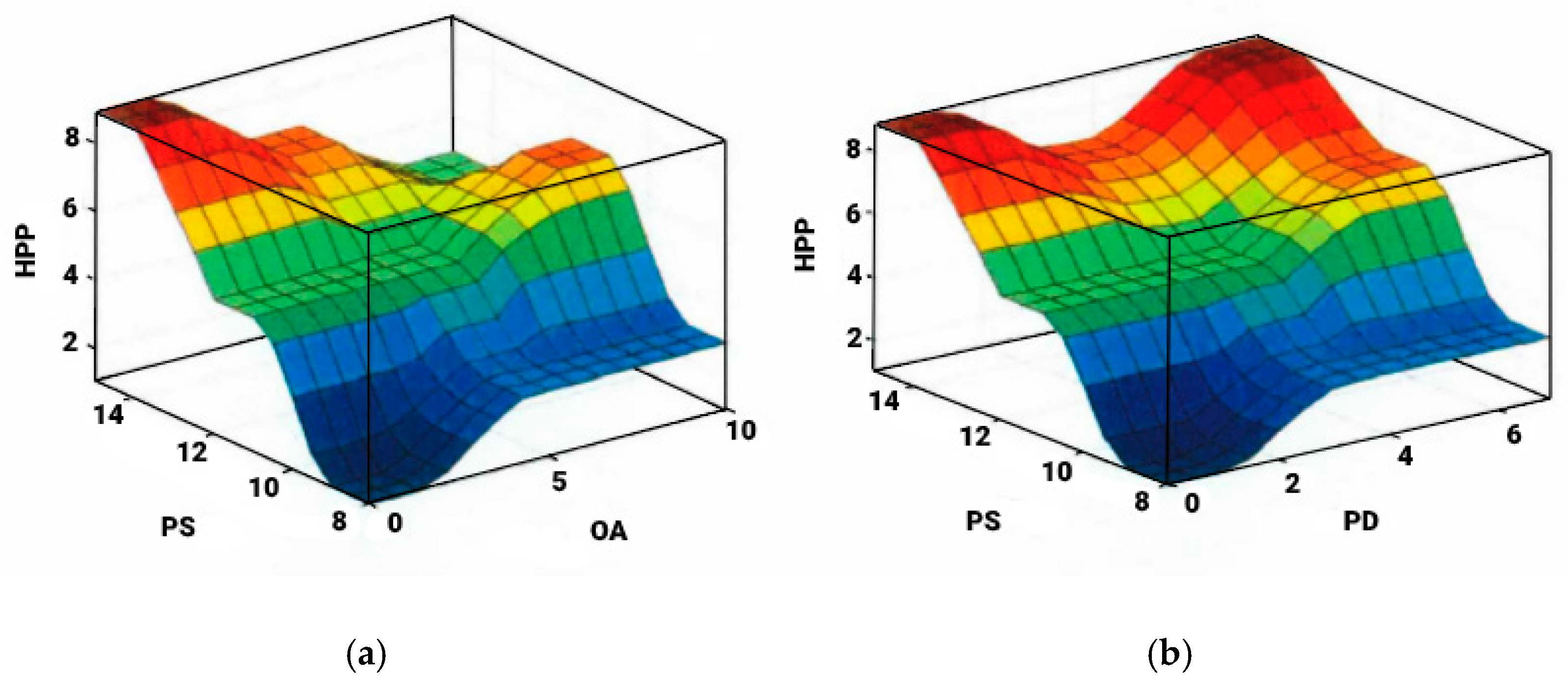
2.1.2. The Model of Fuzzy Reasoning System

In the fuzzy reasoning model, the input variables are the pressure (PS) and operability (OA) of wells and the pressure difference (PD) or differential pressure of adjacent wells on the same pipeline. The output variable is the high-pressure possibility (HPP) that the well belongs to the high-pressure area.

The fuzzy sets and domains of PS, PD, OA and HPP are defined as follows:

(1)

The fuzzy set of PS is (low, middle, high). The domain is (8, 15). The domain value is different for different oil fields or production blocks.

(2)

The fuzzy set of PD is (low, middle, high). The domain is (0, 7). The domain value is different for different oil fields or production blocks.

(3)

The fuzzy set of OA is (low, middle, high). The domain is (0, 10).

(4)

The fuzzy set of HPP is (low, lower, middle, higher, high). The domain is (0, 10). If the fuzzy set of HPP is above higher, it can be included in the high-pressure area.

2.1.3. Design of Fuzzy Reasoning Rules

This reasoning rule is used to judge the possibility that a well belongs to the high-pressure area. Firstly, it is judged by pressure. High-pressure wells must belong to the high-pressure area. Low-pressure wells are judged according to other conditions, such as operability. The second is to judge by pressure difference of adjacent wells connected on the same pipeline. It also depends on operating conditions if the pressure difference is high. The well should still be included in the high-pressure area if pressure is still relatively high, although the pressure difference is low. Some fuzzy logic rules are shown in

Table 1. Fuzzy logic rules.

Rule Number	PS	PD	OA	HPP
1	Low	Low	Low	Low
2	Low	Low	Middle	Low
3	Low	Low	High	Low
4	Low	Middle	Low	Low
5	Low	Middle	Middle	Lower
6	Low	Middle	High	Lower
7	Low	High	Low	Lower
8	Low	High	Middle	Lower
9	Low	High	High	Middle
10	Middle	Low	Low	Middle
11	Middle	Low	Middle	Middle
12	Middle	Low	High	Higher
13	Middle	Middle	Low	Middle
14	Middle	Middle	Middle	Middle
15	Middle	Middle	High	Higher
16	Middle	High	Low	Lower
17	Middle	High	Middle	Higher
l8	Middle	High	High	Higher
19	High	Low	Low	High
20	High	Low	Middle	High
21	High	Low	High	High
22	High	Middle	Low	High
23	High	Middle	Middle	Higher

.

The fuzzy reasoning system is simulated by the fuzzy logic toolbox of MATLAB [23]. The fuzzy regular surface is shown in Figure 1. Fuzzy logic is used to judge the possibility that a well is classified into a high-pressure area. Those with a possible reasoning value greater than 7 can be classified as a high-pressure area. It should be noted that it is not appropriate to divide the whole pipe network into more high- and low-pressure areas.

2.2. A New Adaptive Ant Colony Genetic Hybrid Algorithm

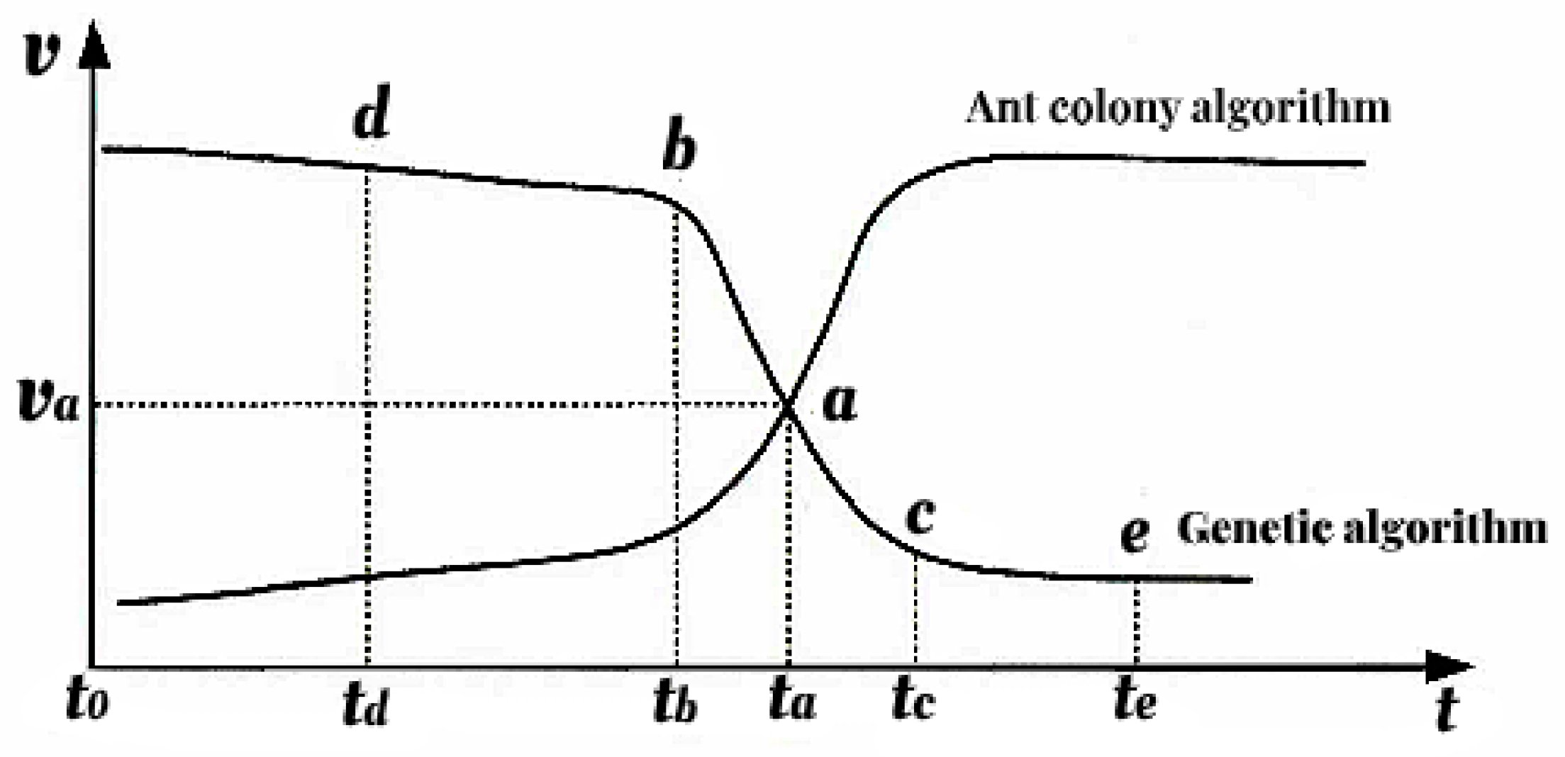
2.2.1. Fusion of the Genetic Algorithm and Ant Colony Algorithm

According to the needs of the optimal operation of the low-pressure network area, we came up with an adaptive ant colony genetic hybrid optimization algorithm, which is better than the ant colony algorithm in time efficiency and genetic algorithm in solving efficiency. The speed-time curve of the two methods is shown in Figure 2. The genetic algorithm has a higher convergence rate to the optimal solution in the initial $t_0-t_a$ period, but the efficiency decreases significantly after $t_a$. On the other hand, the search speed of the ant algorithm in the initial $t_0-t_a$ period is slow due to the lack of pheromone. The speed of convergence to the optimal solution increases rapidly when the pheromone accumulates to a certain intensity after the $t_a$ time [24,25].

The new algorithm has two improvements:

(1)

An adaptive control strategy for pheromone volatilization coefficient is proposed in order to improve the solution efficiency of the ant colony algorithm and prevent the results from falling into the local optimization.

(2)

The maximum and minimum ant systems are introduced to limit the residual pheromones in each subspace to a certain range in order to prevent stagnation and diffusion.

2.2.2. Adaptive Ant Colony Genetic Hybrid Algorithm

Firstly, the solution space is divided. The optimization model of operation parameters is established, whereby the optimization variable is the external water delivery of each pump and the objective function is the minimum energy consumption of the system [26,27].

$$\min f(Q)=\alpha \cdot {\displaystyle \sum _{i=1}^n\frac{(P_{ci}-P_{ri})\cdot q_i}{{\eta }_{pi}{\eta }_{ei}}}$$

(1)

$$l_i\le q_i\le u_i\left(i=1,2,\cdots ,n\right)$$

(2)

The value range of variables in each dimension is divided into N sub-intervals. The length of sub-intervals is:

$$L_i=\frac{u_i-l_i}{N}\left(i=1,2,\cdots ,n\right)$$

(3)

The value range of the j-th sub-interval in the i-th dimension is:

$$\left[l_i+\left(j-1\right)\cdot L_i,l_i+j\cdot L_i\right]\left(i=1,2,\cdots ,n\right)\left(j=1,2,\cdots ,N\right)$$

(4)

The specific steps of the algorithm are as follows:

Step 1. The space of each optimization is divided into N sub-intervals. The length of each sub-interval $L_i$ is calculated. The ant number of each dimension optimization variable is m. The cycle count is kc = 1.

Step 2. m initial solutions $Q_1,Q_2,\cdots ,Q_m$ are randomly generated. The function $f_1,f_2,\cdots ,f_m$ and fitness functions $fitnes{s}_1,fitnes{s}_2,\cdots ,fitnes{s}_m$ are calculated. The sub-intervals to which each component of the m initial solutions belongs are determined. $q_{ki}$ is the i-th dimension component of $q_k$.

If $l_i+\left(j-1\right)\cdot L_i<q_{ki}\le l_i+j\cdot L_i\left(k=1,2,\cdots ,m;i=1,2,\cdots ,n;j=1,2,\cdots ,N\right)$. $q_{ki}$ belongs to the j-th sub-interval. The pheromone for each sub-interval is initialized:

$${\tau }_{ij}={\displaystyle \sum _{k=1}^m\Delta {\tau }_{ij}^k}$$

(5)

$$\Delta {\tau }_{ij}^k=\{\begin{array}{ll}A\cdot fitnes{s}_k& (\mathrm{If}\mathrm{the}\mathrm{solution}\mathrm{of}\mathrm{ant}k\mathrm{falls}\mathrm{into}\mathrm{the}j\text{-}\mathrm{th}\mathrm{subinterwal}\mathrm{of}i\text{-}\mathrm{th}\mathrm{component})\\ 0& \left(\mathrm{else}\right)\end{array}$$

(6)

where $\Delta {\tau }_{ij}^k$ is the information left by ant k in the j-th sub-interval of the i-th component. A is a constant.

The number of ants falling into each sub-interval $Num{1}_{ij}\left(i=1,2,\cdots ,n;j=1,2,\cdots ,N\right)$ is counted $m={\displaystyle \sum _{j=1}^{N}Num{1}_{ij}}$.

Step 3. The number of ants in each sub-interval $Num{2}_{ij}\left(i=1,2,\cdots ,n;j=1,2,\cdots ,N\right)$ is redistributed according to the ratio ${\tau }_{ij}/{\sum }_{j=1}^N{\tau }_{ij}$, $m={\displaystyle \sum _{j=1}^{N}Num{2}_{ij}}$.

Step 4. The removal operation is carried out $\left(Num{1}_{ij}-Num{2}_{ij}\right)$. Ants with poor fitness in the j-th subinterval of the i-dimension are removed and saved in a new list where $Num{2}_{ij}<Num{1}_{ij}$.

Step 5. The move in operation is carried out $\left(Num{2}_{ij}-Num{1}_{ij}\right)$. Ants are moved into the sub-interval from the list of removed ants if $Num{2}_{ij}>Num{1}_{ij}$. Finally, there is a new solution $Q_1^{(1)},Q_2^{(1)},\cdots ,Q_m^{(1)}$.

Step 6. The function $f{1}_1^{},f{1}_2^{},\cdots ,f{1}_m^{}$ and $fitness{1}_1,fitness{1}_2,\cdots ,fitness{1}_m$ of $Q_1^{(1)},Q_2^{(1)},\cdots ,Q_m^{(1)}$ are calculated.

Step 7. The select, cross and mutate genetic evolution of ants in each dimension of sub-interval is carried out. The sub-solutions $Q_1^{(2)},Q_2^{(2)},\cdots ,Q_m^{(2)}$ are generated.

Step 8. The functions $f{2}_1^{},f{2}_2^{},\cdots ,f{2}_m^{}$ and $fitness{2}_1,fitness{2}_2,\cdots ,fitness{2}_m$ of $Q_1^{(2)},Q_2^{(2)},\cdots ,Q_m^{(2)}$ are calculated.

Step 9. $Q_1^{(2)},Q_2^{(2)},\cdots ,Q_m^{(2)}$ and $Q_1^{(1)},Q_2^{(1)},\cdots ,Q_m^{(1)}$ are compared. The new solution $Q_k$ is generated.

$$Q_k=\{\begin{array}{l}{Q}_k^{(2)}\left(f{2}_k<f{1}_k\mathrm{or}fitness{2}_k>fitness{1}_k\right)\\ Q_k^{(1)}\left(else\right)\end{array}$$

(7)

Step 10. Pheromone in the sub-interval of each dimension variable is updated.

$${\tau }_{ij}\left(t+1\right)=\rho \left(t+1\right)\cdot {\tau }_{ij}\left(t\right)+\Delta {\tau }_{ij}$$

(8)

The maximum–minimum ant system is introduced to limit the pheromone to $\left[{\tau }_{\min },{\tau }_{\max }\right]$

$${\tau }_{ij}\left(t+n\right)=\{\begin{array}{l}{\tau }_{\min },if {\tau }_{ij}\left(t\right)\le {\tau }_{\min }\\ {\tau }_{ij}\left(t\right),if {\tau }_{\min }<{\tau }_{ij}\left(t\right)\le {\tau }_{\max }\\ {\tau }_{\max },if {\tau }_{ij}\left(t\right)>{\tau }_{\max }\end{array}$$

(9)

where the adaptive control strategy is adopted for the pheromone volatilization coefficient.

$$\rho \left(t+1\right)=\{\begin{array}{l}C\cdot \rho \left(t\right),if C\cdot \rho \left(t\right)>{\rho }_{\min }\\ {\rho }_{\min },else\end{array}$$

(10)

Step 11. $Num{1}_{ij}$ = $Num{2}_{ij}$. kc = kc + 1.

Step 12. Steps 3–11 are repeated until $\left|f_i-f_{i-1}\right|<\epsilon$. $\epsilon$ is the calculation accuracy, which is taken as 0.01 in this paper. The algorithm flow chart is shown in Figure 3.

2.3. K-Means Algorithm for High Pressure Zone Topology

The K-means algorithm of machine learning belongs to unsupervised learning. The purpose of clustering is to find the potential category of each sample and put the same category sample together. The training sample is $\left\{x^{(1)},\cdots ,x^{(m)}\right\}$. $x^{(i)}\in R^n$ [28,29].

The K-means algorithm is described as follows [30]:

Step 1. K cluster centroids are initialized $\mu =\left\{{\mu }_1,{\mu }_2,\cdots ,{\mu }_k\right\}$, ${\mu }_j\in R^d(1\le j\le K)$. The set of each cluster centroid ${\mu }_j$ is $G_j$.

Step 2. The distance between each sample to be clustered and K cluster centroids is calculated, as is the Euclidean distance between $x_i$ and $u_j$. Each $x_i$ is put into the cluster set, where the nearest cluster centroids.

$$dist\left(x_i,{\mu }_j\right)=\sqrt{{\displaystyle \sum _{o=1}^d{\left(x_{i,o}-{\mu }_{j,o}\right)}^2}}\left(1\le i\le n,1\le j\le K\right)$$

(11)

Step 3. The new centroid is calculated according to the results contained in each cluster set.

$${\mu }_j=\frac{1}{\left|G_j\right|}{\displaystyle \sum _{x_i\in G_j}{x}_i}$$

(12)

Step 4. Algorithm iteration until the cluster centroids remain the same in the two iterations of before and after.

The topological transformation in high-pressure areas is to gather all high-pressure wells into K well clusters and minimize the investment in the waterflooding system. The K clusters, location of the booster station and the high pressure well to which it belongs are finally determined.

3. Results and Discussion

Taking the waterflooding system of the X plant in the Daqing Oilfield as an example, this paper introduces the application of different zones and pressure. The X plant currently includes 10 waterflooding stations, 72 water distribution rooms and 2257 wells; 13–14 pumps are opened. The waterflooding volume is $9\times {10}^4-10\times {10}^4$ m³. The average unit consumption is about 5.80 kWh/m³ every day. This paper developed the program with C++ Builder software to conduct the simulation and analysis.

3.1. Simulation and Analysis of System

After a simulation of the waterflooding system, the waterflooding radius of each station, the pipe network efficiency of each station area and the maximum pressure loss from each station to the end well were determined. The results are shown in Figure 4, Figure 5, Figure 6 and Figure 7.

The energy consumption analysis of the system is shown in Figure 8. Pump energy consumption and pipe network pressure drop are necessary albeit useless, comprising 22.8% of the total energy. Pressure differences of the pump pipe and well pipe are similarly wasteful and useless, comprising 19.9% of the total energy. The useful energy injected into the well is 57.3%. Therefore, the energy saving of the system must start with reducing the pressure difference of the pump pipe and well pipe.

The flooding pressure distribution of wells is shown in Figure 9. The pressure of wells in the northeast corner and in the east and west zone is relatively high. They are basically 12.0–13.5 MPa. A few wells are 13.5–15.0 MPa. The pressure of other wells is relatively low. They are below 12.0 MPa and some even below 10 MPa. In the system, the average pump pressure is 16.6 MPa. The average pipe pressure of wells is 15.4 MPa. The average oil pressure of wells is only 11.8 MPa. The well pipe pressure difference reaches 3.6 MPa. The serious loss at the well valve is the main contradiction of the high energy consumption.

In addition, due to the uneven pressure distribution in each block of the waterflooding system of the X oilfield, the pump start-up operation and layout are not very reasonable. The wellhead pressure in the middle, east and eastern transition zone of Xing 1~3 is basically between 12.0 MPa and 13.5 MPa, and a few wellhead pressures are between 13.5 MPa and 15.0 MPa; the pressure in the middle and west is basically below 12.0 MPa, the pressure of the western transition zone is higher than 12.0 MPa and the pressure of a few wells is higher than 13.5 MPa. If the overall depressurization method is adopted to reduce the well pipe differential pressure, the waterflooding wells with high flooding pressure demand will not meet the waterflooding demand.

3.2. Different Zone and Pressure of System

According to system pressure distribution, the distinguishing of the pressure in the system are carried out. The pipe network is divided into high- and low-pressure areas by a trunk line valve. The whole pressure reduction in the low-pressure area is carried out to reduce the well pipe pressure difference. The pump is taken down a step to reduce the pump pipe pressure difference. Figure 10 shows the high- and low-pressure area divided by fuzzy logic theory. The larger area on the left is the low-pressure area. The smaller area on upper right corner is the high-pressure area.

The layout of the pipe network, the location of the highway and the feasibility of the operation should be considered in the different pressure calculation using fuzzy logic theory. The waterflooding trunk lines are cut off from lines 1–2 to lines 4–4 by the valve. The exact cut-off position is shown in Figure 11.

3.3. Operation Effect of Low-Pressure Area

There are 8 waterflooding stations and 18 pumps in the low-pressure area. Four waterflooding pumps of Xing-16, Xing-20 and Xing-22 stations were reduced grade. A frequency conversion pump was turned on in Xing-19 station. Pump characteristic curve fitting is carried out using the big data method. The fitted characteristic curves are shown in Figure 12.

The adaptive optimization method is used for the optimization calculation of the pumps in the low-pressure area. The optimization results are shown in

Table 2. Contrast result of before and after operation scheme optimization on low-pressure waterflooding system.

Station Number	Available Pump Numbers	Current Operation Scheme		Optimized Operation Scheme
		Running Pump Number	External Volume of Water (m3/d)	Running Pump Number	External Volume of Water (m3/d)
1#	1, 2, 3	1, 2	81,066,008	1	9129
2#	1, 2	2	6753	1	6749
3#	1, 2, 3	3	6677	3	9508
4#	1, 2, 3	1	6714	2	8000
5#	1, 2, 3	1	9293	1	9503
6#	1, 2, 3	2	10,981	2	10,996
7#	1, 2, 3	2, 3	75,446,939	2, 3	76,297,501

and

Table 3. Energy consumption of the low-pressure area before and after different pressure in the X oilfield.

Low Pressure Area	Volume of Water Daily (m3/d)	Average Pump Pressure (MPa)	Average Pipe Pressure (MPa)	Unit Consumption (kWh/m3)
before different pressure	63237	16.23	15.68	5.69
after different pressure	61411	15.36	14.69	5.48

.

After the different pressure and step-down measures, it can be seen from the production data that the average pump pressure decreased to 0.87 MPa, the average pipe pressure decreased to 0.99 MPa, the unit consumption decreased to 0.27 kWh/${\mathrm{m}}^3$ and the efficiency of the system increased 2–3 percentage points. A good energy saving effect was achieved.

3.4. Operation Effect of High-Pressure Area

There are two waterflooding stations and five pumps in the high-pressure area. The booster station layout of the high-pressure wells and the pumping scheme of other wells in the high-pressure area are determined with system simulation and K-means calculation.

The booster stations of 97 high-pressure wells (>13.5 MPa) in the high-pressure area were arranged. The contour coefficient method was used to determine the best number of booster K stations. We achieved K = 4. At the same time, the construction of the booster station or single well booster can be determined by comparing and analyzing the cost. The booster station layout is shown in Figure 13 and Figure 14. The affiliation of high-pressure wells and booster stations is shown in

Table 4. Affiliation of high-pressure wells and booster stations.

Name of Booster Station	Booster Station 1	Booster Station 2	Booster Station 3	Booster Station 4
Number of high-pressure wells	17	3	41	36
Volume of water in flooding (m3)	640	135	1160	1780
Well pressure (MPa)	13.6–14.2	13.8–14.1	13.8–14.6	13.6–14.5

.

One pump of Xing-18 station and two pumps of Xing-17 station are turned on for other wells in the high-pressure area. The average pump pressure in the high-pressure area decreased from 16.13 MPa to 15.90 MPa after operation. The average pipe pressure decreased from 15.63 MPa to 15.40 MPa. The average unit consumption decreased from 5.64 kWh/m³ to 5.19 kWh/m³. The results are shown in

Table 5. Energy consumption of the high-pressure area before and after different pressure in the X oilfield.

	Daily Waterflooding (m3/d)	Average Pump Pressure (MPa)	Average Pipe Pressure (MPa)	Pump Water Consumption (kWh/m3)
Before the downgrade pump is put into operation	23,800	16.13	15.63	5.64
After the downgrade pump is put into operation	25,772	15.90	15.40	5.19

.

4. Conclusions

The mixed flooding of high–low pressure wells of the waterflooding system leads to an increase in the overall energy consumption and complicates the optimizing operation of the pipe network. This paper classified high- and low-pressure wells from the perspective of different pressure with fuzzy logic theory so as to accurately match flooding pressure, reduce overall pressure and improve the operating efficiency of the system.

(1)

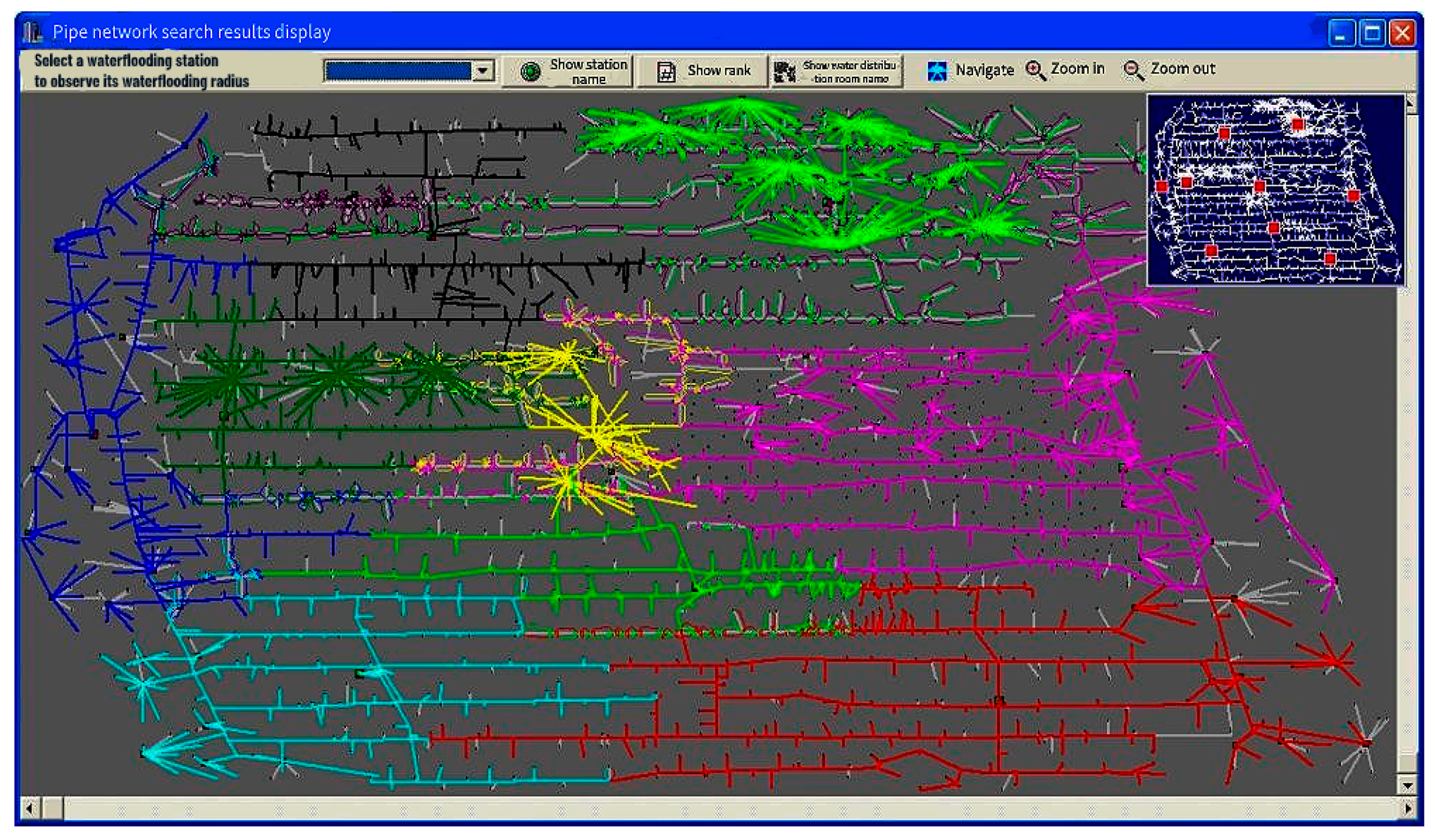
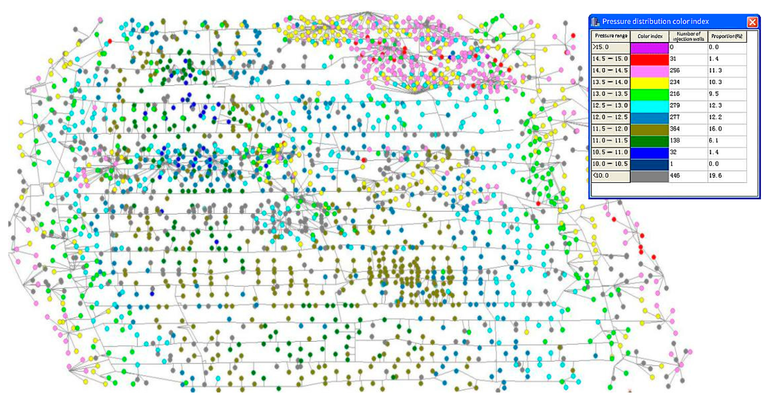
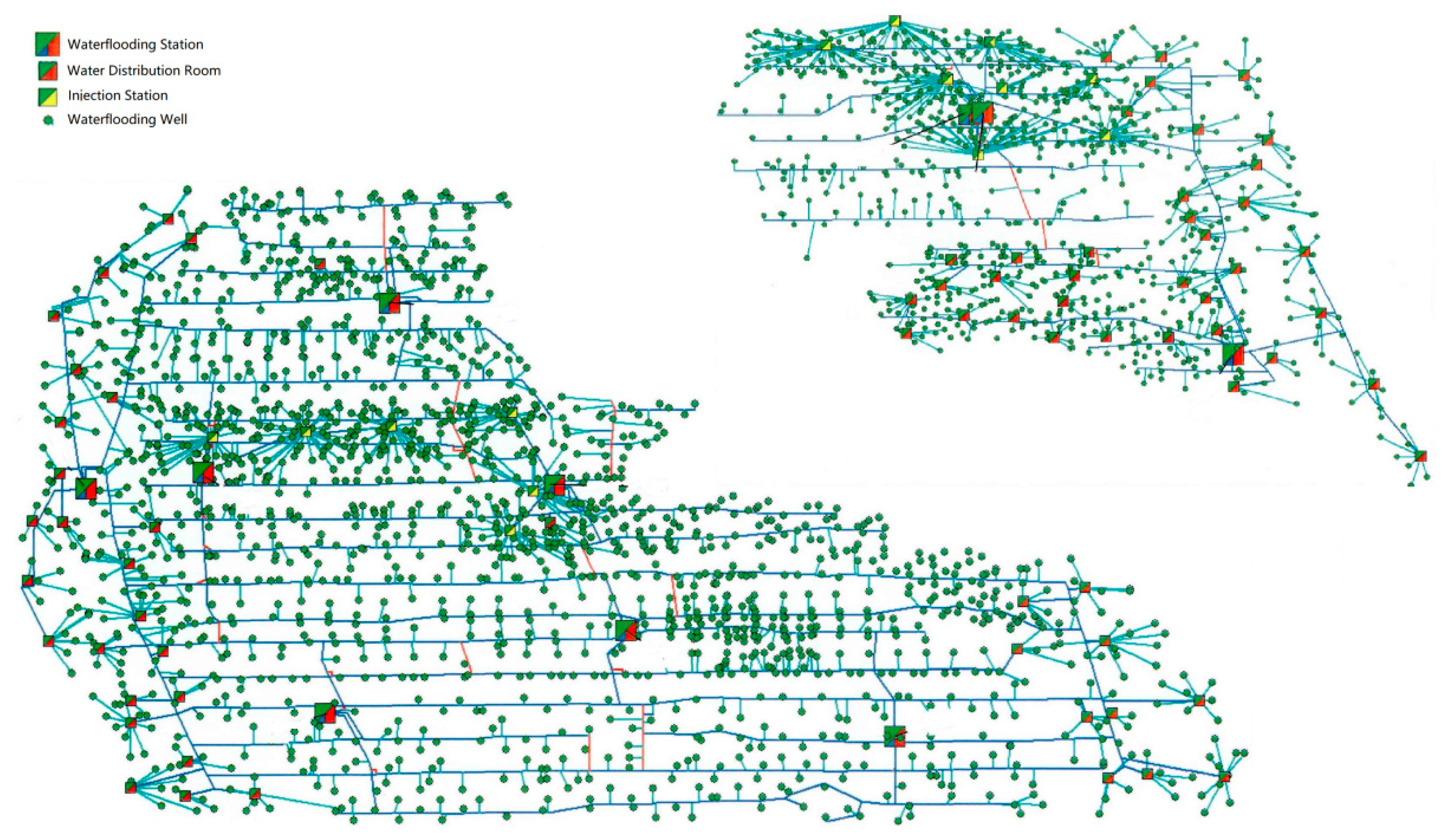
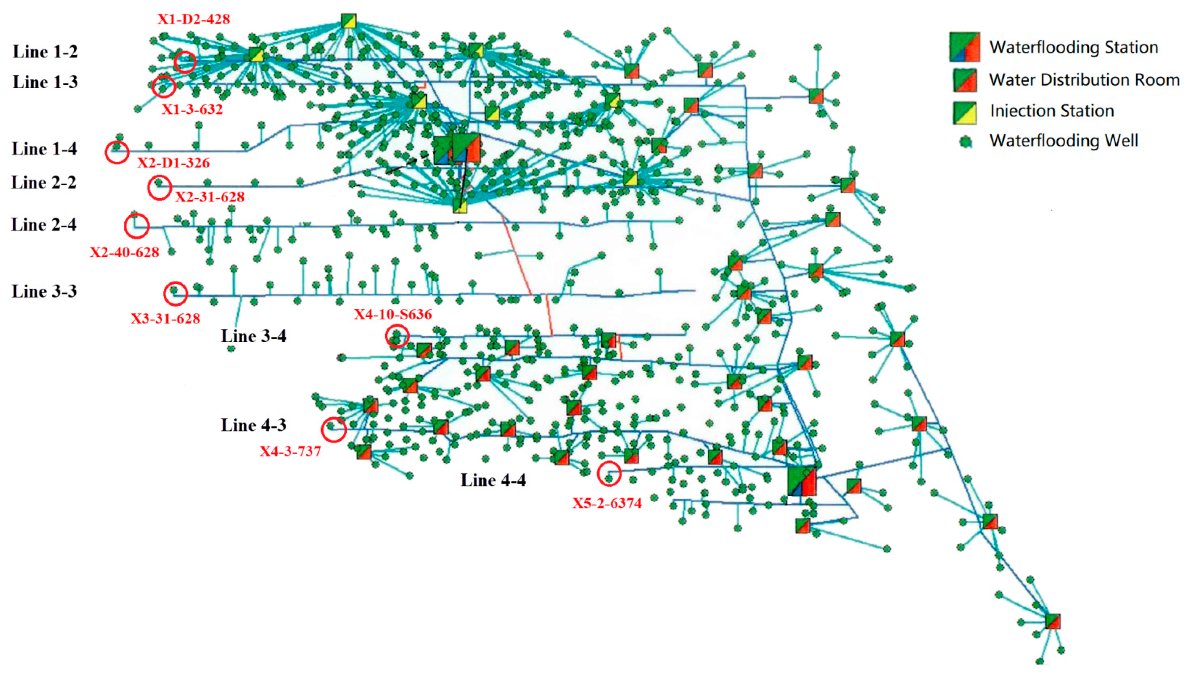
According to the characteristics of mixed distribution for high–low pressure wells in oilfields and based on the fuzzy logic theory, a different pressure model is established; well pressure, the pressure difference of adjacent wells and operability are its variables. The fuzzy logic theory domain and reasoning rules are established. As an example, the different pressure design of the waterflooding system is carried out with the X oilfield including 2200 wells and 10 waterflooding stations in a site in China. It is proven that the theory and method can effectively divide wells into high–low pressure areas through simulation and application research.

(2)

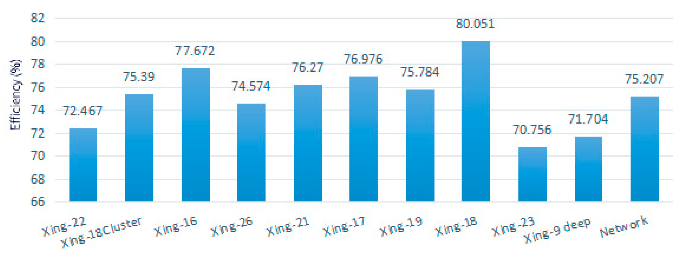
A new adaptive ant colony genetic hybrid algorithm is proposed based on the analysis of the genetic algorithm and ant colony algorithm and the characteristics of operation optimization for the waterflooding system. This method is used to calculate the operation optimization problem after separating pressure. The energy saving effect is remarkable through the application of the optimization results in the X oilfield. Its unit consumption decreased to 0.27 kWh/${\mathrm{m}}^3$ and the efficiency of the system increased 2–3 percentage points.

(3)

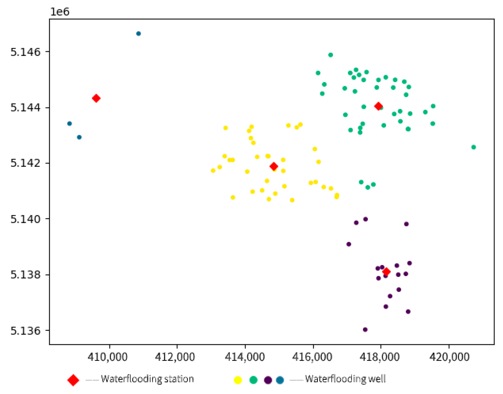
The K-means algorithm is introduced into the station layout in the high-pressure area. The objective function is to minimize the investment of the waterflooding system. The flooding requirements of the waterflooding wells are the constraints. The model is established and solved. The results show that the energy saving effect of the high-pressure area is remarkable after the renovation. Its unit consumption decreased to 0.45 kWh/${\mathrm{m}}^3$.

(4)

The research results show the new method of classifying high–low pressure wells has great significance for solving high–low pressure mixed flooding in old oilfields and the increase in system energy consumption from the perspective of different pressure.

References

1. Naevdal, G.; Brouwer, D.R.; Jansen, J.D. Waterflooding Using Closed-loop Control. Comput. Geosci. 2006, 10, 37–60. [Google Scholar] [CrossRef]
2. Tang, L.; Li, J.; Lu, W.; Lian, P.; Wang, H.; Jiang, H.; Wang, F.; Jia, H. Well Control Optimization of Waterflooding Oilfield Based on Deep Neural Network. Geofluids 2021. [Google Scholar] [CrossRef]
3. Seddiqi, K.N.; Mahdi, Z. Application of waterflooding technique to the Angut oilfield in the northern part of Afghanistan. J. Pet. Explor. Prod. Technol. 2018, 8, 939–946. [Google Scholar] [CrossRef] [Green Version]
4. Zhang, H.; Liang, Y.; Zhou, X.; Yan, X.; Qian, C.; Liao, Q. Sensitivity analysis and optimal operation control for large-scale waterflooding pipeline network of oilfield. J. Pet. Sci. Eng. 2017, 154, 38–48. [Google Scholar] [CrossRef]
5. Zhou, X.; Liang, Y.; Xin, S.; Di, P.; Yan, Y.; Zhang, H. A MINLP model for the optimal waterflooding strategy and operation control of surface waterflooding pipeline network considering reservoir characteristics. Comput. Chem. Eng. 2019, 129, 106512. [Google Scholar] [CrossRef]
6. Liang, H.B.; Li, M.; Tan, X.Q. Discussion on simulated annealing algorithm for optimal scheduling of water supply system. Water Supply Drain. 1999, 25, 30–33. [Google Scholar]
7. Orr, C.H.; Ulanicki, B.; Rance, J.P. Computer control of operations at a large distribution systems. J. Am. Water Wastewater Assoc. 1992, 84, 68–74. [Google Scholar] [CrossRef]
8. Liu, W.G. Research on modeling and optimization of large centrifugal pumping station system in oilfield. China Equip. Eng. 2007, 5, 10–12. [Google Scholar]
9. Li, L.; Zhang, C.G.; Lin, J.H.; Li, H.B. Optimal scheduling of pumping station based on cell exclusion double population genetic algorithm. Control. Theory Appl. 2004, 1, 63–69. [Google Scholar]
10. Yang, P.; Ji, X.H.; Shi, W.W. An improved genetic algorithm for optimal scheduling of pumping stations considering variable frequency speed regulation. J. Yangzhou Univ. 2002, 5, 67–70. [Google Scholar]
11. Ning, Y.B.; Ming, Z.F.; Zhong, Y.R. Principle and realization of variable frequency speed regulation and constant pressure water supply system. J. Xi’an Univ. Technol. 2001, 17, 305–309. [Google Scholar]
12. Ilich, N.; Simonovic, S.P. Evolutionary Algorithm for Minimization of Pumping Cost. J. Comput. Civ. Eng. 1998, 12, 232–240. [Google Scholar] [CrossRef]
13. Hou, D.Y.; Sun, S.G. Optimal scheduling of water supply pump station based on genetic algorithm. J. Shandong Univ. (Eng. Ed.) 2003, 33, 25–28. [Google Scholar]
14. Yao, Z.Q. Discussion on several issues in frequency control and constant pressure water supply. J. Xi’an Highw. Univ. 1997, 17, 80–82. [Google Scholar]
15. Yang, X.X.; Li, L.; Lin, J.H. Research on optimal control of water supply pump station based on genetic algorithm. J. Appl. Basic Eng. Sci. 1999, 7, 209–214. [Google Scholar]
16. Yang, P.; Ji, X.H.; Shi, W.W. Optimal scheduling of pumping stations based on genetic algorithm. J. Yangzhou Univ. 2001, 4, 72–74. [Google Scholar]
17. Chen, H.; Liu, Z.Y.; Shi, W.W. Optimal scheduling of water supply pump station based on simulated annealing algorithm. Drain. Irrig. Mach. 2003, 21, 34–37. [Google Scholar]
18. Guan, X.J.; Wei, L.X.; Yang, J.J. Optimization model of oilfield waterflooding system operation scheme based on hybrid genetic algorithm. Chin. J. Pet. 2005, 26, 114–117. [Google Scholar]
19. Yang, J.J.; Liu, Y.; Wei, L.X.; Zhan, H. Double coding hybrid genetic algorithm for optimal scheduling of pump station in multi-source waterflooding system. J. Autom. 2006, 32, 154–160. [Google Scholar]
20. Wei, L.X.; Liu, Y.; Sun, H.Z. Optimization of operation and scheduling of waterflooding system in multi-source oilfield. Pet. Extr. Technol. 2007, 29, 59–62. [Google Scholar]
21. Yang, J.J.; Liu, Y.; Wei, L.X.; Zhan, H.; Zeng, W. Operation optimization of waterflooding system based on dual coding genetic algorithm. Pet. Mine Mach. 2006, 35, 8–11. [Google Scholar]
22. Rodriguez, A.X.; Aristizábal, J.; Cabrales, S.; Gómez, J.M.; Medaglia, A.L. Optimal waterflooding management using an embedded predictive analytical model. J. Pet. Sci. Eng. 2022, 208, 109419. [Google Scholar] [CrossRef]
23. Zhang, M. The adjustment method of centrifugal pump and its energy consumption analysis. Coal Technol. 2005, 24, 18–20. [Google Scholar]
24. Guo, Z.Y.; Reynolds, A.C.; Zhao, H. Waterflooding optimization with the INSIM-FT data-driven model. Comput. Geosci. 2018, 22, 745–761. [Google Scholar] [CrossRef]
25. Zhang, R.J. Research on Intelligent Analysis and Operation Optimization Technology of Waterflooding System Production State; Northeast Petroleum University: Daqing, China, 2011. [Google Scholar]
26. Zhang, K.; Zhao, X.G.; Chen, G.D.; Zhao, M.J.; Wang, J.; Yao, C.J.; Sun, H.; Yao, J.; Wang, W.; Zhang, G.D. A double-model differential evolution for constrained waterflooding production optimization. J. Pet. Sci. Eng. 2021, 207, 109059. [Google Scholar] [CrossRef]
27. Marotto, T.A.; Pires, A.P. Mathematical modeling of hot carbonated waterflooding as an enhanced oil recovery technique. Int. J. Multiph. Flow 2019, 115, 181–195. [Google Scholar] [CrossRef]
28. VATTANI; ANDREA. K-means requires exponentially many iterations even in the plane. Discret. Comput. Geom. 2011, 45, 596–616. [Google Scholar] [CrossRef] [Green Version]
29. INABA; MARY; Katoh, N.; Imai, H. Applications of weighted Voronoi diagrams and randomization to variance-based k-clustering. In Proceedings of the Tenth Annual Symposium on Computational Geometry, New York, NY, USA, 6–8 June 1994. [Google Scholar]
30. Wu, F. Introduction to Artificial Intelligence: Models and Algorithms; Higher Education Press: Beijing, China, 2020. [Google Scholar]
Figure 1. Fuzzy logic surface. (a) Fuzzy regular surface PS, OA-HPP. (b) Fuzzy regular surface PS, PD-HPP.
Energies 15 01444 g001
Figure 2. Speed–time curve of the genetic algorithm and ant algorithm.
Energies 15 01444 g002
Figure 3. Algorithm flow chart.
Energies 15 01444 g003
Figure 4. The waterflooding radius of the system.
Energies 15 01444 g004
Figure 5. Maximum pressure loss from the station to end well.
Energies 15 01444 g005
Figure 6. Pipe network efficiency of each station area.
Energies 15 01444 g006
Figure 7. Pipeline flow velocity analysis.
Energies 15 01444 g007
Figure 8. Analysis of pressure and energy consumption in the X plant.
Energies 15 01444 g008
Figure 9. Pressure distribution of flooding wells.
Energies 15 01444 g009
Figure 10. Different pressure diagram of the system.
Energies 15 01444 g010
Figure 11. Cut-off position of the pipe network.
Energies 15 01444 g011
Figure 12. Big data fitting scatter plot. (a) H-Q curve of 3 pump of Xing-24 station; (b) η-Q curve of 3 pump of Xing-24 station; (c) η-Q curve of 1 pump of Xing-7 station; (d) H-Q curve of 1 pump of Xing-7 station.
Energies 15 01444 g012
Figure 13. Clustering results.
Energies 15 01444 g013
Figure 14. Layout of booster stations.
Energies 15 01444 g014