An Improved Partial Shading Detection Strategy Based on Chimp Optimization Algorithm to Find Global Maximum Power Point of Solar Array System

Abstract

A PV system’s operation highly depends on weather conditions. In case of varying irradiances or load changes, there is a power mismatch between various modules of the PV array. This power mismatch causes instability in the output of the PV system and deteriorates the overall system efficiency. To overcome instability and lower efficiency problems, and to extract maximum power from the PV system, various maximum power point tracking (MPPT) techniques are employed. The success of these techniques depends on the identification of the actual operating conditions of the system. This article proposes a hybrid maximum power point tracking (MPPT) technique that is capable of efficiently differentiating between uniform irradiance, non-uniform irradiance, and load variations on the PV system. Based on the identified operating conditions, the proposed method uses modified perturb and observe (Modified P&O) to cope with uniform irradiance variations and chimp optimization algorithms (ChOA) for non-uniform conditions to track the oscillation free maximum power-point. The proposed method is implemented and verified using a 4 × 3 PV array model in MATLAB Simulink software. Different cases of uniformly changing irradiance and non-uniformly changing irradiance are applied to test the performance of the proposed hybrid technique. The load varying conditions are performed by applying a variable load resistor. The authenticity of the proposed hybrid technique is critically evaluated against the well-known and most widely used optimization techniques of modified perturb and observe (Modified P&O), particle swarm optimization (PSO), flower pollination algorithm (FPA), and grey wolf optimization (GWO). The results demonstrate the superiority of the proposed technique in oscillation-free tracking of global maximum power point (GMPP) in a minimum tracking time of 0.4 s and 0.15 s, and steady-state MPPT efficiency of 96.92% and 99.54% under uniform and non-uniform irradiance conditions, respectively.

1. Introduction

Most conventional energy resources rely on fossil fuels, which are costly, diminishing, and pollute the atmosphere. Moreover, existing energy resources are unable to meet increasing energy demands. Consequently, the need for cost-effective, renewable, more efficient, and environmentally friendly sources of energy has been boosted. As a result of improved technology, falling prices, and supporting policies for PV installation, the present decade has seen a large proportion of PV usage as compared to any other form of renewable energy [1].

Although solar PVs are a promising candidate, having economical and environmental benefits, they are highly dependent and suffer from unfavorable weather patterns (i.e., soiling, aging of modules, and tree, building, or cloud shadows). In addition, temperature variations and irregular irradiance have adverse effects. In particular, partial shading (PS) caused by clouds has a severe effect on PV array output.

As a result of PS, there is an unequal distribution of irradiance on different modules of the PV array. This irregular irradiance pattern creates a mismatch of power between various modules, imposing a multi-peak condition on the PV curve. Additionally, fluctuations in the output characteristics decrease the overall efficiency of the PV system [2].

Initial studies introduced the concept of array reconfiguration for countering the mismatch effects. A competence square (CS) technique is used in [3] for the physical rearrangement of PV modules in total-cross-tied (TCT) configuration under PS conditions. The knight pattern array reconfiguration method is suggested by [4] for maximum power extraction by equalizing shading distribution on various P V modules under partial shading conditions. In [2,5,6] various reconfiguration topologies (i.e., series, series-parallel, total-cross-tied, bridge-linked, honey-comb, physical relocation of the module with fixed electrical connections (PRM-FEC), SuDoKu, and Magic Square (MS)) are considered and compared. Although total-cross-tied (TCT) configuration exhibits better performance, increased circuit complexity and cost are its major drawbacks. Furthermore, physical relocation of modules or switching of electrical connections is an additional problem for reconfiguration methods under frequently changing weather patterns.

Another approach to improving PV performance using conventional MPPT methods (i.e., perturb and observe (P&O) [7], incremental conductance (IC) [8], hill climbing (HC) [9], ripple correlation control (RCC) [10], fractional open circuit (FOC) [11], fractional short circuit (FSC) [12], etc.) has been evaluated in [13]. In [14], a variable step size and fixed step size-based incremental conductance MPPT approach is suggested. The simulation and experimental verification show better performance under variable step conditions; however, it still has excessive oscillations in its output characteristics. In [15], an efficient method of direct power transmission from PV to the grid is implemented by a combination of multiple P&O and boost inverter topology. The proposed approach is successful in effectively tracking MPP. A hybrid MPP tracking method using linear tangent and Neville interpolation (LT-NI) is applied to track the maximum power of the PV system [16]. Despite having efficient performance under uniform irradiance change, the proposed technique fails to track the MPP during partial shading cases. Consequently, the assessment of these conventional techniques indicates outstanding performance under uniform irradiance change; however, in the case of partial shading, these algorithms are stuck in the local peaks, unable to track the global peak (i.e., optimum operating point). Hence, conventional MPPT methods cannot be relied upon for real-time control of PV systems under unpredictable climate conditions.

The recent technological advances and research focus have proposed soft computing and metaheuristic algorithms to cope with the problems of PS. The key advantage is improved efficiency and reduced computational burden. The author in [17] proposed a crow search algorithm (CSA)-based optimization technique for MPPT and compared it with particle swarm optimization (PSO) and P&O. The analysis shows improved performance of CSA as compared to traditional PSO and P&O methods. The article in [18] deduces some rules to determine shading occurrence and suggests a flower pollination algorithm (FPA) for MPPT in severe shading situations. In [19], optimal operating point is tracked using the firefly algorithm (FA). The results demonstrate the superiority of FA over PSO and P&O in terms of tracking speed and efficiency. A hybrid method is adopted in [20] for oscillation-avoidance-based MPPT using a combination of P&O and genetic algorithm (GA). Although the technique is successful in approaching the MPP, its tracking period contains huge oscillations, causing a slow convergence speed in reaching the MPP. The Spline-MPPT approach proposed in [21] claims to find maximum power under uniform and partial shading cases by using a small number of sample points. Using a smaller number of sample points compromises the accuracy. Moreover, utilizing the Spline-MPPT method under uniform conditions can be complicated, as MPP can be easily determined by simple modification in conventional P&O algorithms. A recently published article [22] has applied the parabolic-assumption algorithm to track GMPP under partial shading situations using a single current sensor. The simulation and experimental results verify the effectiveness of the proposed method. A very effective skipping-adaptive P&O algorithm is designed in [23], which enhances the MPP tracking speed by avoiding scanning of certain regions of the PV curve. The grey wolf optimization (GWO)-based control technique is validated in [24], and results are compared with the most widely used conventional P&O and improved PSO (IPSO) methods. The comparison shows that the proposed GWO method outperforms both P&O and IPSO. In [25], a collaborative swarm algorithm (CSA) is adopted to improve the tracking speed and efficiency of MPP tracking by employing the excellent features of PSO, Jaya, and ACO-NUP collaboratively. Another recent strategy to counter the partial shading effects using a most valuable player algorithm (MVPA) is assumed in [26]. The performance of the proposed method is compared with the most widely used PSO and modified Jaya algorithm; although it exhibits comparatively better tracking capability, its MPP tracking duration still has high undershot oscillations. Furthermore, in [27], GWO-FC technique is employed for mitigating the oscillations around GMPP. A search-space-skipping-based MPPT method is proposed in [28] to track GMPP under rapidly varying partial shading conditions. The authenticity and effectiveness of this approach are evaluated against maximum power trapezium (MPT) and flower pollination algorithm (FPA). The comparison indicates the superiority of the proposed method as it efficiently skips the unnecessary region from scanning for MPP, which ultimately contributes to fast convergence and improved efficiency. Recently, an enhanced cuckoo search algorithm was recommended in [29] for GMPP tracking under partial shading conditions. In [30], a dynamic particle MPPT approach is recommended. This method evaluates the transient characteristics of the dc-dc boost converter and uses the idea of dynamic sample time to achieve fast and improved tracking of MPP under random shading patterns. A flying squirrel search optimization (FSSO)-based method is used in [31], which effectively reaches the GMPP under non-uniform irradiance variation. An advantage of FSSO is having very small tracking oscillation, while steady-state conditions have no oscillations.

The comprehensive literature review and comparative analysis of reconfiguration methods, conventional methods, and metaheuristic-algorithm-based MPPT methods conclude that the latter is the most suitable approach to deal with complex partial shading conditions on PV systems. Even though metaheuristic techniques have outstanding performance in partial shading conditions, most of these methods have some limitations (i.e., complexity, increased tuning parameters, slow convergence speed, and large tracking and steady-state oscillations).

The main research gap in the existing literature is the problems and limitations associated with global maximum power point tracking (GMPPT) techniques while dealing with uniform irradiance change, partial shading, and load variations. The existing problems are listed as follows:

(a)

Rarely discussed and inefficient classification/identification of uniform, partial shading, or load-varying conditions.

(b)

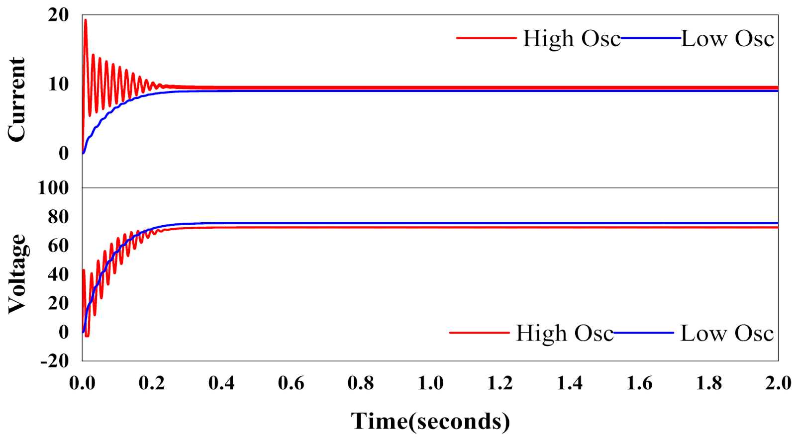
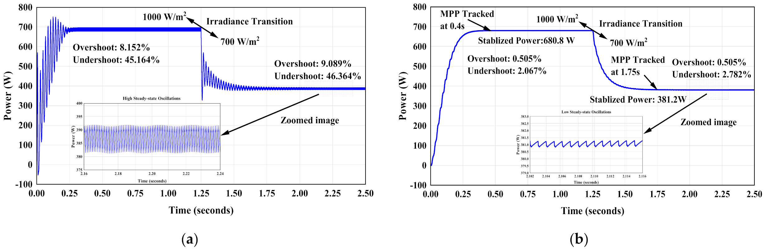
Slow convergence speed and large tracking and steady-state oscillations.

(c)

Unsuccessful tracking of GMPP due to inefficient triggering of MPPT algorithms caused by incorrect detection of actual operating conditions of the PV system.

These issues can be resolved by combining the benefits of conventional and metaheuristic methods to design a hybrid method [17]. To avoid unnecessarily triggering between algorithms, it is extremely important to identify the occurrence of partial shading and differentiate it from the uniform change of irradiance [18]. The detection of partial shading conditions (PSC) is crucial for the efficient design of the MPPT controller. Most of the studies consider large power or voltage change as a result of partial shading; however, in reality, this is not always true.

To accurately identify the actual operating conditions of a PV system, this paper proposes an efficient approach to differentiate between uniform irradiance, non-uniform irradiance, and load variations. Moreover, based on the identified operating conditions, the proposed hybrid technique uses modified P&O for oscillation-free MPP tracking under uniform irradiance change. The chimp optimization algorithm (ChOA) [32], having the advantages of fewer tuning parameters, high convergence speed, and negligible tracking oscillations, is employed to extract global maximum power point (GMPP) in the case of non-uniform irradiance and load variations. Additionally, ChOA results are compared with well-known modified perturb and observe (Modified P&O), particle swarm optimization (PSO), flower pollination algorithm (FPA), and grey wolf optimization (GWO) MPPT methods.

The novel contributions and improvement of this research work are as follows:

• Identification of actual operating conditions of the PV system, as well as discrimination between uniform irradiance change, non-uniform irradiance change, and load variations.
• Observing and distinguishing the combined effect of load and irradiance variations.
• Oscillation-free transient and steady-state GMPP tracking under uniform and non-uniform conditions using modified P&O and chimp optimization algorithms, respectively.
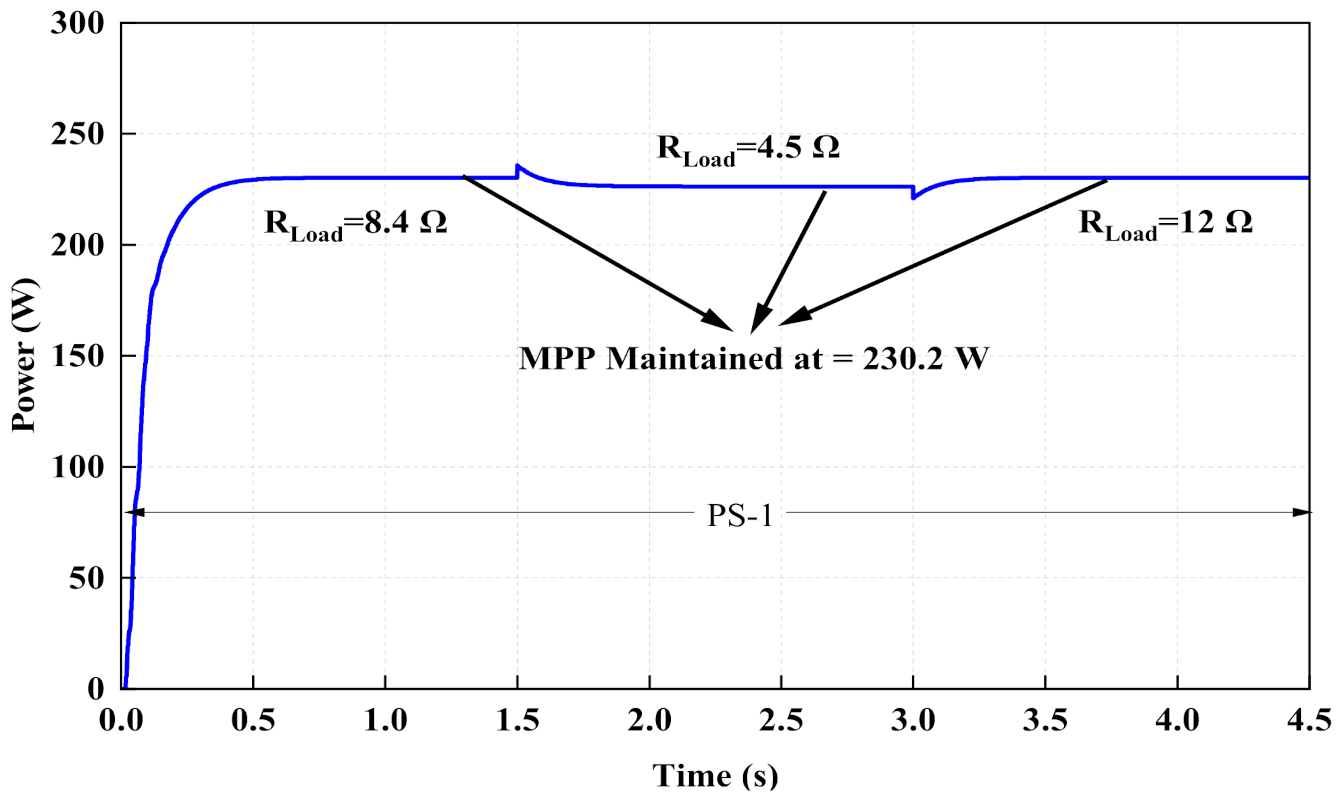
• Efficiently maintaining GMPP under load variations to verify the robustness of the proposed methodology.
• The superiority of the proposed technique is confirmed through comparative analysis with modified P&O, PSO, GWO, and FPA MPPT methods.

The remaining part of the paper is structured as follows: Section 2 explains the PV system modeling. Section 3 presents and classifies operating conditions. The proposed hybrid GMPPT methodology is detailed in Section 4. The results and discussions are in Section 5. Finally, the conclusion and future work are in Section 6 and Section 7, respectively.

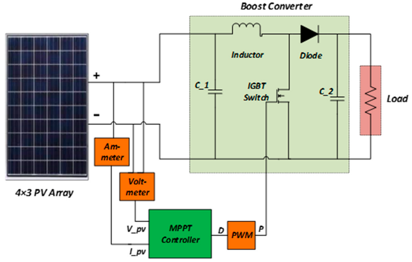
2. PV System Modelling

The output power of a solar array system is highly dependent on the effectiveness of the cells used in the PV module. A PV cell is a fundamental part of the solar system [33], so there is an emphasis on its efficient design. In the literature, a variety of models have already been presented (i.e., single-diode model, two-diode model, and three-diode model). Each of these has non-uniform behavior under changing weather patterns. The comprehensive analysis of the above three models under uniform as well as partial shading situations has been shown in [34]. PV characteristics of the array system under different shading cases showed the superiority of the single-diode model over other models (two-diode and three-diode). Moreover, due to the simplicity and involvement of fewer parameters, the single-diode model has been extensively used in PV module modeling. A schematic diagram of the single-diode model used in this paper is shown in Figure 1.

The ideal model of a single diode consists of a current source connected in parallel with a diode. The equivalent model comprising a series and a shunt resistor is shown in Figure 1. V-I characteristics of the single-diode model are analyzed using MATLAB/Simulink tools:

Mathematically,

$$I=I_{pv}-I_d-\left(\frac{V_{out}+I{R}_s}{R_{sh}}\right)$$

(1)

where

$$I_d=I_{sat}\left[e^{\left(\frac{q\left(V_{out}+I{R}_s\right)}{aKT}\right)}-1\right]$$

(2)

Now, by substituting I_d in (1):

$$I=I_{pv}-I_{sat}\left[e^{\left(\frac{q\left(V_{out}+I{R}_s\right)}{aKT}\right)}-1\right]-\left(\frac{V_{out}+I{R}_s}{R_{sh}}\right)$$

(3)

Here, Equation (3) shows the overall output current equation for the single-diode model, where

‘I_pv’ is photo-generated current,

‘I_sat’ is diode reverse saturation current,

‘I’ is output current,

‘V_out’ is the voltage at the output terminal,

‘a’ is the ideality factor of the diode,

‘q’ denotes electron charge (1.6 × 10⁻¹⁹ C),

‘K’ is Boltzmann constant (1.3806503 × 10⁻²³ J/K),

‘T’ is the temperature in Kelvin,

R_s and R_sh are series and shunt resistances, respectively. It is evident from Equation (3) that the single-diode model needs estimation of the following five parameters: I_pv, I_sat, R_s, R_sh, and a.

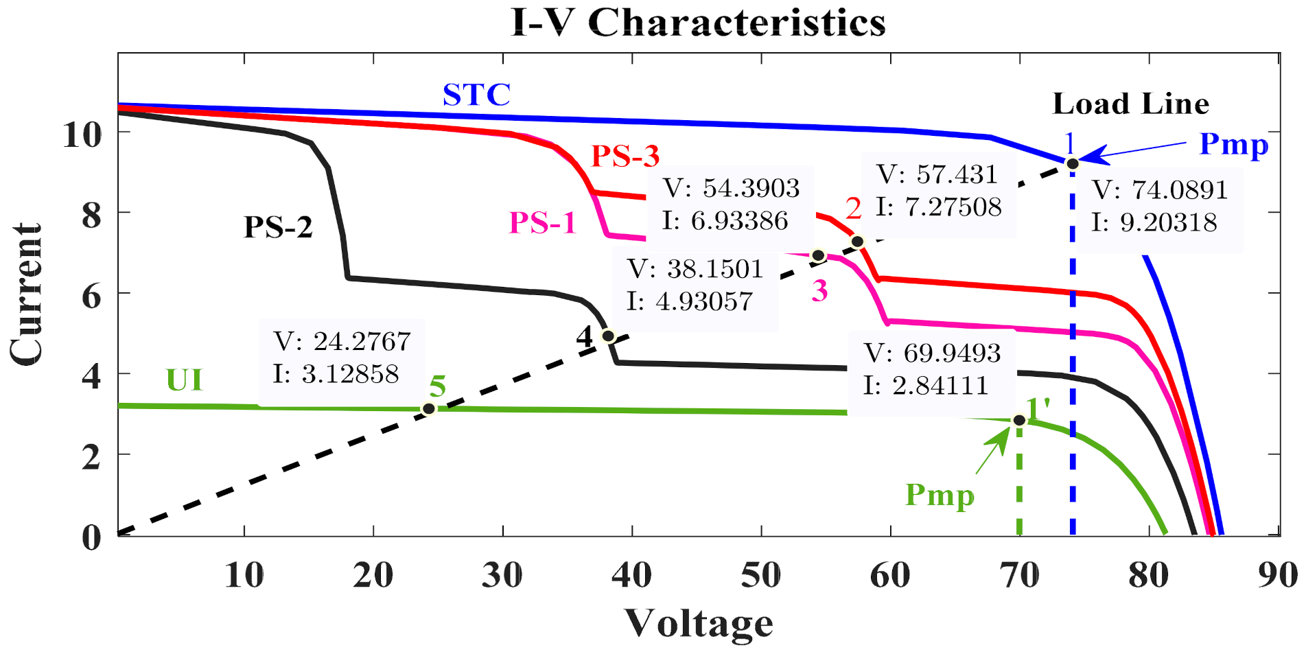
3. Operating Conditions

3.1. Classification of Uniform and Non-Uniform Irradiance Variation

The I-V characteristics of a 4 × 3 S-P connected PV array are shown in Figure 2. Initially, all modules are fully irradiated at 1000 W/m², and the PV system is operating at maximum power point (P_mp) 1. At point 1, voltage is V_mp = 74.09 V, and current I_mp = 9.203 A. However, due to uniform irradiance change, all modules are now receiving 300 W/m² irradiance, and the system’s new operating point (OP) is shifted to 1’, having voltage of V_mp = 69.95 V and current of I_mp = 2.841 A. By carefully observing points 1 and 1’ on STC and UI curves, respectively, it is evident that during uniform irradiance change there is only one peak, known as the maximum power peak. Moreover, the voltage variation (∆V_mp ≅ 5%) is very small, while contrarily, current is reduced significantly.

In the case of partial shading, PS-1 in Figure 2, the maximum power operating point is at OP-3, having current of I_mp = 6.933 A and voltage of V_mp = 54.39 V. Now, the irradiance level changes, and OP will move to a new position, OP-2, on PS-3, with an increase in voltage (V_pv2 = 57.43 V) and current (I_pv2 = 7.275 A) as compared to V_mp and I_mp of PS-1.

Again, the variation of irradiance causes the OP to be shifted to OP-4 on PS-2 with a decrease in voltage (V_pv3 = 38.15 V) and current (I_pv3 = 4.931 A) as compared to V_mp and I_mp of PS-1. Consequently, non-uniform irradiance change can be identified if Equation (4) is satisfied.

$$\left.\begin{array}{c}{V}_{pv}\left(i\right) >V_{mp} and I_{pv}\left(i\right) >I_{mp}\\ Or\\ V_{pv}\left(i\right) <V_{mp} and I_{pv}\left(i\right) <I_{mp}\end{array}\right\}$$

(4)

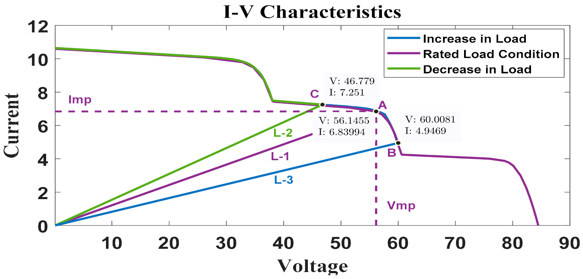
3.2. Identification of Load Variations

Load-varying conditions (LVC) are investigated by examining the OP behavior on the PS curve of Figure 3. At the rated load condition, the system is operating at maximum power point A with voltage V_mp = 56.15 V and current I_mp = 6.84 A. An increase in load causes the OP to move from point A on load line L-1 to point B on L-3. This new OP has a voltage of V_pv3 = 60.01 V more, while the current (I_pv3 = 4.947 A) is less as compared to V_mp and I_mp at point A. However, a decrease in load forces the OP to shift to point C on L-2 causing a decrease in voltage (V_pv2 = 46.78 V) and an increase in the current (I_pv2 = 7.251 A) in comparison to V_mp and I_mp at point A. As a result, load variations can be identified if the expression in (5) has been satisfied [35].

$$\left.\begin{array}{c}{V}_{pv}\left(i\right) <V_{mp} and I_{pv}\left(i\right) >I_{mp}\\ Or\\ V_{pv}\left(i\right) >V_{mp} and I_{pv}\left(i\right) <I_{mp}\end{array}\right\}$$

(5)

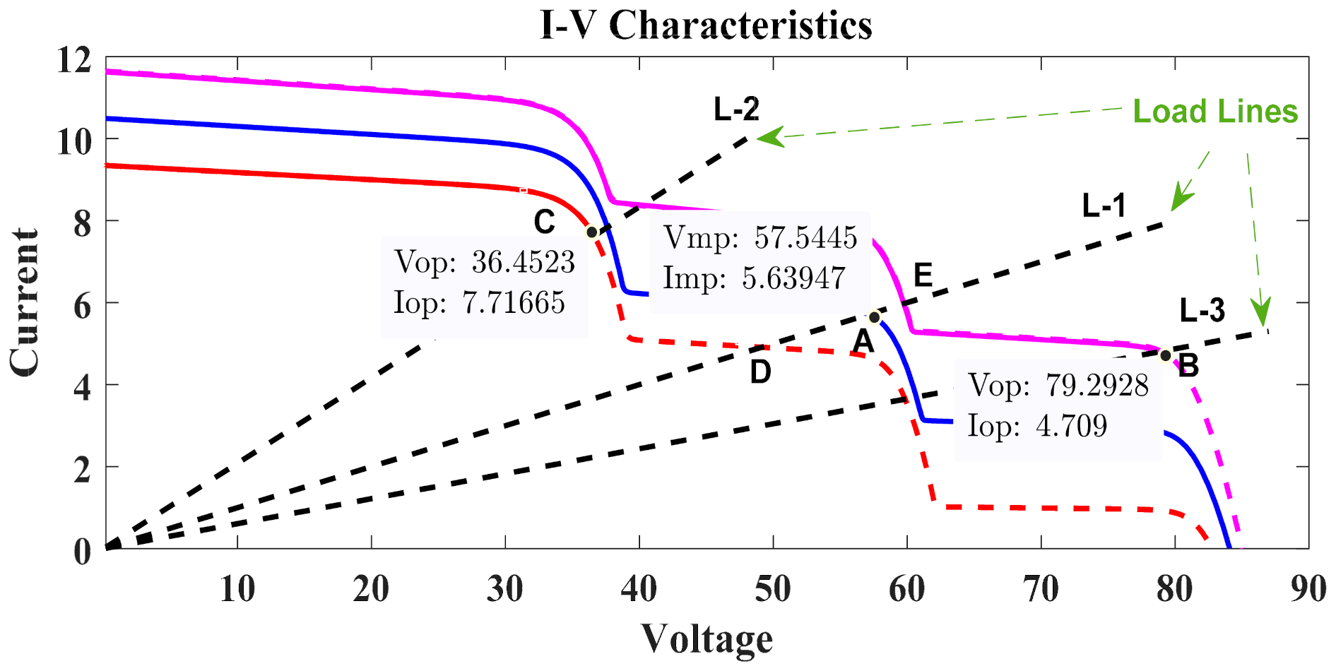
3.3. Combined Effect of Load and Irradiance Variations

In real-time scenarios, there is always a possibility of variation in load and irradiance at the same time. To tackle such a situation, modifications in (4) and (5) are inevitable. In particular, two cases are considered for dealing with the combined effect of load and irradiance variations in this work. Initially, the PV system is operating at maximum power point A as shown in Figure 4, with voltage V_mp = 57.5445 V and current I_mp = 5.63947 A. In case 1, let us suppose there is a sudden decrease in load, and at the same moment, irradiance is also decreased. As a result, the OP moves away from maximum power point A to point C for change in load and irradiance simultaneously. The accurate identification of the case 1 condition can be expressed mathematically as follows:

$$\left.\begin{array}{c}\Delta V=V_{op}-V_{mp}<0\\ \Delta I=I_{op}-I_{mp}>0\end{array} \right\}$$

(6)

In case 2, the load is increased, and at the same time, there is an increase in irradiance, causing OP to relocate from point A to point B, as shown in Figure 4. This type of load and irradiance change can be determined as follows:

$$\left.\begin{array}{c}\Delta V=V_{op}-V_{mp}>0\\ \Delta I=I_{op}-I_{mp}<0\end{array} \right\}$$

(7)

Additionally, the concept of slope variation is used to differentiate between irradiance and load change. In Figure 4, the slope of load line-1 (L-1) does not change (i.e., m_A = m_D = m_E = 0.1) with the variation of irradiance level. However, in the case of a change of load, the load line L-1 shifted to L-2 or L-3. As a result, the slope variation can be used to identify the occurrence of load change.

Mathematically,

$$\left.\begin{array}{c}\Delta m=0; Irradiance Variation\\ \Delta m>0;Decrease in Load\\ \Delta m<0;Increase in Load \end{array} \right\}$$

(8)

where

$$\Delta m=m_{new}-m_{mp}$$

(9)

Here, $m_{mp}$ represents the slope of the load line at the maximum power point A, while $m_{new}$ is a new slope after the change of load/irradiance.

4. Proposed Hybrid GMPPT Methodology

The proposed hybrid technique in this work uses the modified perturb and observe, along with the recently developed chimp optimization algorithm (ChOA) [27]. To accomplish the objective of efficient global maximum power point (GMPPT) tracking under uniform irradiance change, non-uniform irradiance change (i.e., partial shading), and load variations, the actual operating conditions of a PV system are identified first. After that, based on the identified situation, modified P&O or ChOA are employed for successful tracking of maximum power point (MPP). The proposed method is divided into three phases, as shown in the flowchart of Figure 5. These phases are explained here as follows.

4.1. Identification of Operating Conditions

In the first phase, the critical analysis of I–V characteristics is done considering various irradiance and load conditions. As shown in Figure 5a, if normalized voltage change is below 5%, the PV system is considered as operating in uniform irradiance conditions (UIC), as already explained in Section 3. The modified P&O is employed for oscillation-free tracking of MPP under uniformly changing irradiance. On the other hand, if normalized voltage change is more than 5% (i.e., the threshold for uniform irradiance change is crossed), the system is assumed to be operating in non-uniform conditions. This situation occurs due to the intermittent nature of solar irradiance or under-changing loads or both. This research detects the combined effect of load and irradiance variation according to Equations (6) and (7) and mitigates their effects individually. For individually tackling the load and irradiance variations, the expression in (8) is used. The load variations are simply dealt with by using the duty cycle compensation method to track back the exact MPP [30].

Upon detection of load variations, the algorithm updates its duty cycle as follows:

$$D_{GMPP\_updated}=\frac{\sqrt{\gamma }}{1+\sqrt{\gamma }}$$

(10)

and

$$\gamma =\frac{I_{GMPP}}{V_{GMPP}}\times \frac{V_L}{I_L}\times \frac{D_{GMPP}{}^2}{{\left(1-D_{GMPP}\right)}^2}$$

(11)

Here, V_L and I_L are voltage and current under load-varying conditions, while GMPP of V, I, and D are the system’s optimal operating point values before the occurrence of load variations.

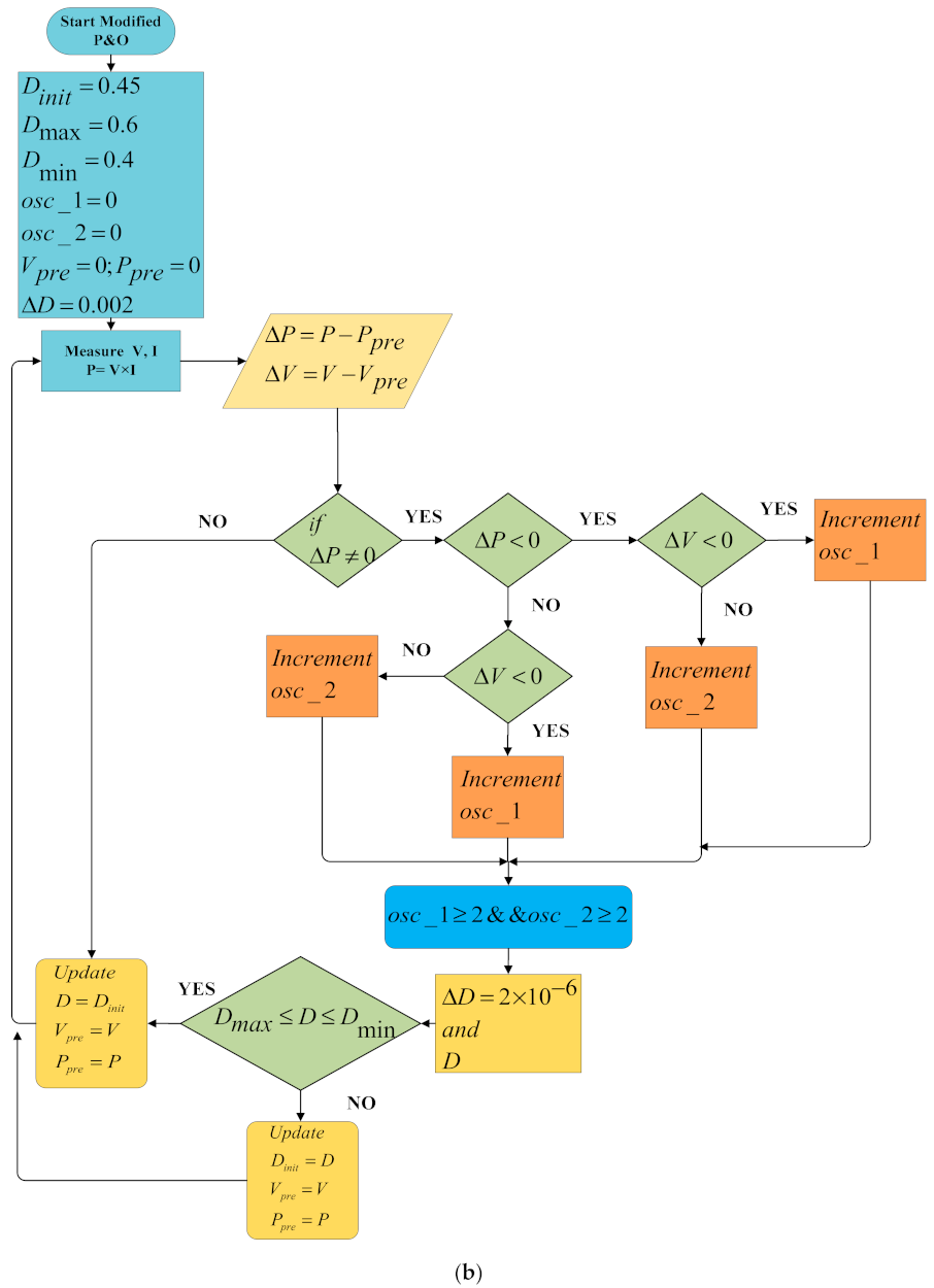
4.2. Oscillation-Free Tracking of MPP Using Modified Perturb and Observe under UIC

To ensure the optimal operation of the PV system under uniform irradiance change, the proposed technique makes use of a modified version of the conventional perturb and observe algorithm. The prime objective is to eliminate the initial and steady-state oscillations and improve the tracking time to reach the MPP under uniformly changing irradiance conditions. The algorithm starts by assigning initial values to the variables.

The upper and lower duty-cycle thresholds are set to 0.60 and 0.40, respectively. These values are set to ensure MPP lies between them. The algorithm initiates with an initial duty cycle of 0.45 and scans the PV curve with a perturbation step of 0.002. The initial voltage (V_pre = 0) and power (P_pre = 0) are defined as previous voltage and previous power and set to zero value. Similarly, the oscillation counters osc_1 and osc_2 are set to zero. The voltage and current of the PV system are measured using measurement devices, and power is calculated. These PV voltages (V) and power (P) values are compared to previously initialized voltage (V_pre) and power (P_pre). If power change is zero ($\Delta \mathrm{P}=0$), the algorithm updates the ‘D’, ‘V_pre’, and ‘P_pre’ values and starts the process again. However, if the change of power ($\Delta \mathrm{P}\ne 0$) is non-zero, the algorithm tracks the MPP and checks for the possibility of steady-state oscillations. If both voltage and power change are negative, the oscillation counter 1 (osc_1) will be incremented by 1. However, a positive change of voltage value causes the oscillation counter 2 (osc_2) to be incremented. On the other hand, if the changes of both voltage and power are positive, the oscillation counter 2 (osc_2) will be incremented, while a positive change of power and negative change in voltage value increments the oscillation counter 1 (osc_1). The algorithm calculates and compares the power and voltage values and checks for osc_1 and osc_2. If the oscillation counter 1 and 2 both have values of 2 or greater, the algorithm considers this as oscillations around the MPP. In the case of oscillations, the perturbation step size is further reduced to minimize the steady-state oscillations. The upper and lower bound duty-cycle values reveal that the finalized duty-cycle ‘D’ is the required value for an oscillation-free steady-state condition. The ‘D_init’, ‘V_pre’_, and ‘P_pre’ values are updated accordingly, as shown in the flowchart of Figure 5b. These upper and lower duty-cycle thresholds define the MPP region and help to avoid the divergence problem.

4.3. Chimp Optimization Algorithm (ChOA)

The increased complexity of array configuration topologies and uncertain weather patterns reinforced the need for an efficient metaheuristic optimization technique. In this paper, the recently evolved chimp optimization algorithm is used to counter the complex irradiance variation conditions. Unlike other optimization techniques, ChOA has the dynamic property of group formation. In this strategy, chimps are divided into four independent groups, and each group has its special characteristics. These individual features of each group help to achieve a common goal more efficiently in the minimum possible time. The four groups of chimp are named attackers (A), barriers (B), chasers (C), and drivers (D) [32]. The mathematical formulation of ChOA for the proposed optimization problem is shown in the flowchart of Figure 5c and described as follows.

Mathematical Formulation of ChOA

In case of non-uniform irradiance conditions (i.e., partial shading), ChOA uses its strategy of driving and chasing the neighborhood of a global maximum operating point in terms of voltage, as below.

$$\chi = \left|\rho V_{mp\_STC}\left(i\right)-\delta V_{pv}\left(i\right)\right|$$

(12)

$$V_{pv}\left(i+1\right) =V_{mp\_STC}\left(i\right)-\sigma .\chi$$

(13)

Here, ‘i’ is iteration number, and ‘$\chi$’ is the distance between actual voltage and desired operating point voltage, while ‘$\sigma$’, ‘$\delta$’, and ‘$\rho$’ shows the coefficient vectors. $V_{mp\_STC}$ is the maximum power point voltage at standard test conditions, and $V_{pv}$ is the measured voltage value during non-uniform irradiance variation.

The coefficient vectors can be calculated as suggested by [32].

$$\sigma =2\beta n_1-\beta$$

(14)

$$\rho =2n_2$$

(15)

$$\delta =chaotic\_value$$

(16)

Here, ‘$\beta$’ reduced non-linearly from 2.5 to 0 during the iteration process. While ‘$n_1$’ and ‘$n_2$’ are random vectors in the range of 0–1. In the end, ‘$\delta$’ is a chaotic vector determined based on various chaotic maps. To track the optimal operating point of the PV array under partial shading conditions, the ChOA approach uses its four chimp groups (i.e., attackers, drivers, chasers, and barriers). Based on the convergence criteria, each chimp group updates its position according to the best chimp’s locations.

This can be further illustrated with the help of Equations (12) and (13) as follows:

$$\left.\begin{array}{c}{\chi }_A=\left|{\rho }_1.V_A\left(i\right)-{\delta }_1.V_{pv}\left(i\right)\right|\\ {\chi }_B=\left|{\rho }_2.V_B\left(i\right)-{\delta }_2.V_{pv}\left(i\right)\right|\\ {\chi }_C=\left|{\rho }_3.V_C\left(i\right)-{\delta }_3.V_{pv}\left(i\right)\right|\\ {\chi }_D=\left|{\rho }_4.V_D\left(i\right)-{\delta }_4.V_{pv}\left(i\right)\right|\end{array} \right\}$$

(17)

and

$$\left.\begin{array}{c} V_1=V_A\left(i\right)-{\sigma }_1.\left({\chi }_A\right); V_2=V_B\left(i\right)-{\sigma }_2.\left({\chi }_B\right) \\ V_3=V_C\left(i\right)-{\sigma }_3.\left({\chi }_C\right); V_4=V_D\left(i\right)-{\sigma }_4.\left({\chi }_D\right)\end{array}\right\}$$

(18)

Now, the best voltage after updating each chimps position is as follows:

$$V_{pv}\left(i+1\right)=\frac{V_1+V_2+V_3+V_4}{4}$$

(19)

In Equation (15), the ‘$\rho$’ vector is a random variable that assigns weights for the MPP to reinforce ($\rho$ > 1) or lessen ($\rho$ < 1) the effect of MPP location in the determination of distance in Equation (16). It helps avoid trapping in local optima and enhances the stochastic behavior of the ChOA technique. The thresholds $\mu$ < 0.5 and |$\sigma$| < 1 ensure convergence towards the global maximum power point (GMPP); however, |$\sigma$| > 1 forces chimps to diverge and globally explore more space. Moreover, the flexible tuning of the ‘$\rho$’ and ‘δ’ vectors allows for local optima avoidance and faster convergence simultaneously.

5. Results and Discussions

To verify the proposed hybrid GMPPT technique, a MATLAB Simulink model was designed using a simple boost converter. The schematic diagram of the proposed model is shown in Figure 6. The design specifications of the boost converter are given in

Table 1. Boost converter specifications.

Parameter	Description/Value
Capacitors [C_1, C_2]	[10 µF, 470 µF]
Inductance	13 mH
Load Resistance	8.4 Ohm
Switching Frequency	1000 Hz

The series-parallel configuration topology is utilized to ensure optimum performance of the 4 × 3 PV array. A user-defined PV module having P_mp = 57.377 W, V_oc = 21.4 V, I_sc = 3.58 A, V_mp = 18.1 V, and I_mp = 3.17 A, as given in

Table 2. Rating of user-defined PV module at STC, T = 25 °C, and irradiance = 1000 W/m².

Parameters	Values at Standard Test Condition(STC)
Power at MPP (Pmp)	57.377 W
Current at MPP (Imp)	3.17 A
Voltage at MPP (Vmp)	18.1 V
Short Circuit Current (Isc)	3.58 A
Open Circuit Voltage (Voc)	21.4 V

, is used for simulation. Moreover, the sampling time of the proposed control technique is selected as 0.5 ms. The expression in (20) is used to determine the steady-state MPPT efficiency of the proposed technique. Different patterns of uniform irradiance and partial shading are applied to validate the performance of the proposed method. The proposed technique differentiates between uniform and non-uniform irradiance variation based on the conditions defined in the flowchart of Figure 5a and uses the MPPT tracking algorithm accordingly. Three cases are considered to authenticate the proposed system’s performance under uniform irradiance change conditions.

$${ɳ}_{\mathrm{ss}}=\frac{\mathrm{Stablized} \mathrm{Power}}{\mathrm{Rated} \mathrm{Power}}\times 100$$

(20)

Here, ‘${ɳ}_{\mathrm{ss}}$’ is steady-state MPPT efficiency.

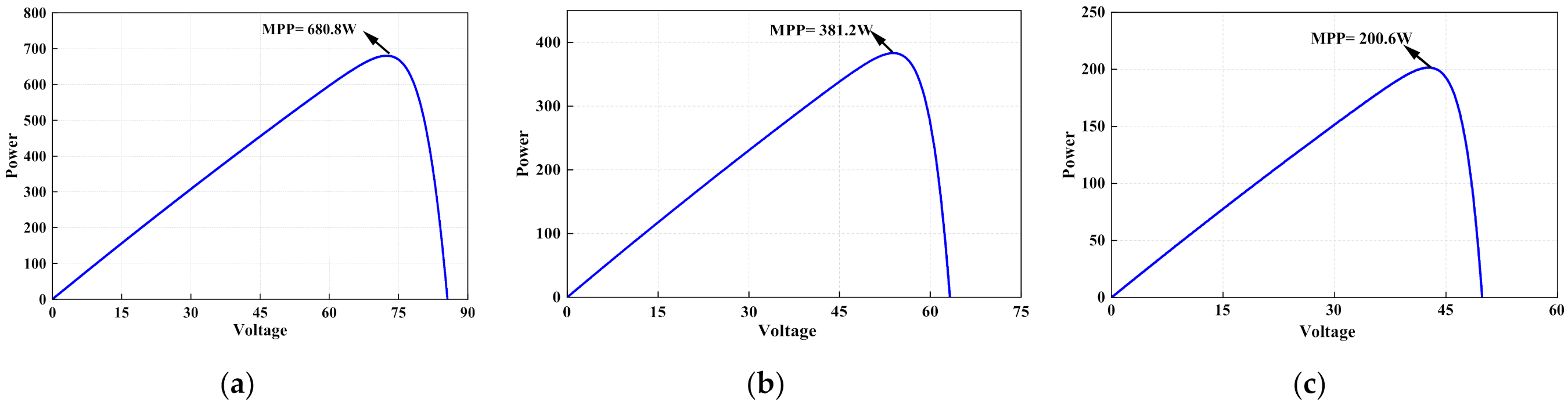
5.1. Uniform Irradiance Conditions

5.1.1. Standard Test Condition (STC)

Initially, the PV array is fully irradiated (1000 W/m²), and according to the flow chart of Figure 5a, the PV system is operating under the uniform irradiance condition; thus, the modified P&O algorithm is initialized to track the exact MPP with reduced oscillations under the steady-state condition as explained in Section 6. Figure 7a,b shows the output power characteristics at standard test condition (i.e., 1000 W/m², 25 °C) with a rated power of 688.524 W. The power curve in Figure 7a has large initial and steady-state oscillations. The highest spike has a value of 751.9 W, which is 72.9 W more than the actual steady-state value of 679 W. These oscillations have an overshoot of 8.152%, while undershoot is 45.164%. These high oscillations destabilize the PV system and reduce its overall efficiency. To overcome these undesirable fluctuations, the proposed modified P&O triggers with the initial perturbation step of ∆D = 0.002, and as it reaches the vicinity of MPP and identifies oscillations, it starts to further reduce the perturbation size to minimize the oscillations around MPP and stabilize the power. The output power curve in Figure 7b proves the validity of the proposed modified P&O’s performance in reducing the high initial and steady-state oscillations. The MPP is tracked in just 0.4 s with a steady-state efficiency of 98.87%. The highest spike, in this case, is the same as steady-state stabilized power of 680.8 W, while overshoot and undershoot values are reduced to 0.505% and 2.067%, respectively. Similarly, voltage and current characteristics with high oscillations (without P&O) and low oscillations (with modified P&O) are shown in Figure 8. While, The PV curves of uniform irradiance cases considered in this study are shown in Figure 9.

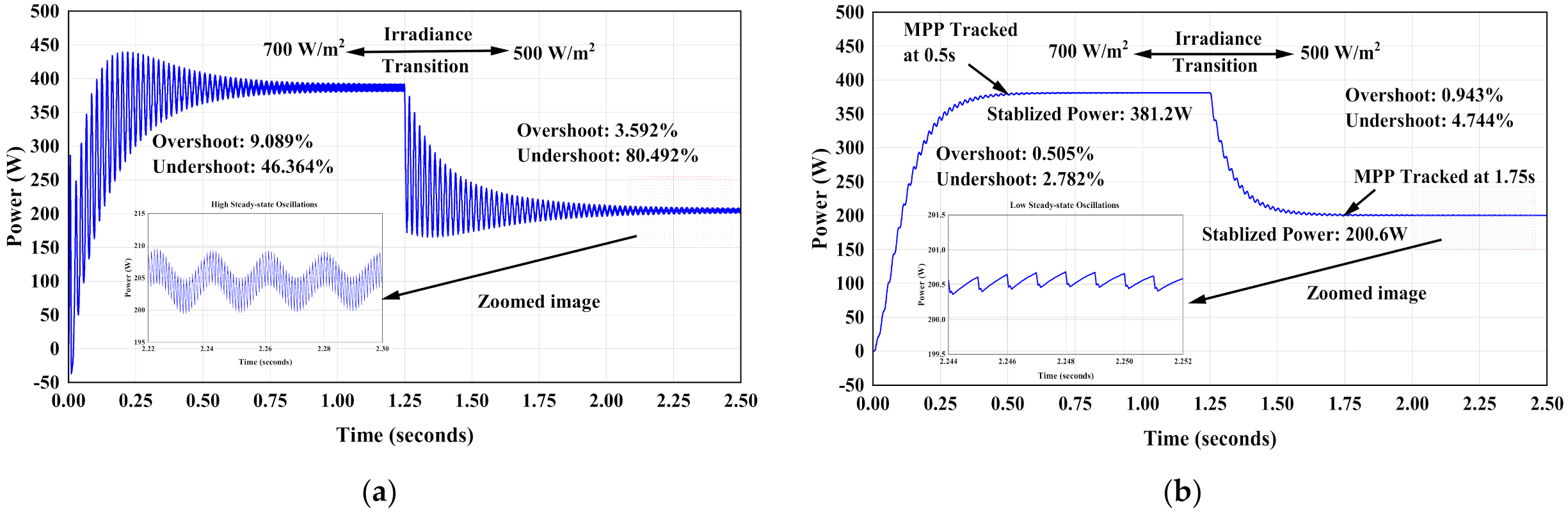
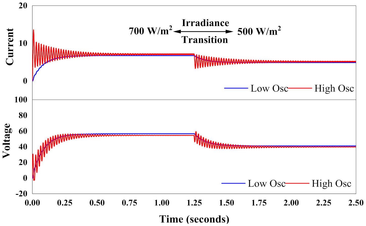
5.1.2. Irradiance Transition (STC→UI-1)

In this case, the irradiation level changes from STC to uniform irradiance 1 (UI-1) at 700 W/m², with a rated power of 401.1 W. This uniform irradiance transition accompanies high initial and steady-state oscillations, having an overshoot of 8.152% and 9.089% and undershoot of 45.164% and 46.364% before and after the irradiance change, respectively, as shown in Figure 10a. As the irradiation value changes at 1.25 s from STC to UI-1, the algorithm identifies it as the uniform irradiance variation and reinitializes modified P&O to track MPP with reduced initial and steady-state oscillations. As the irradiation value changes at 1.25 s from STC to UI-1, the algorithm identifies it as the uniform irradiance variation and reinitializes modified P&O to track MPP with reduced initial and steady-state oscillations. The output power characteristics in Figure 10b confirm that the MPP is tracked at 0.4 s and 1.75 s before and after the irradiance change with a steady-state efficiency of 96.95%. Moreover, overshoot values are decreased to 0.505%, and undershoot values are at 2.067% and 2.782% before and after the irradiance transition, respectively. A similar improvement can be seen in output voltage and current characteristics (Figure 11) by employing the proposed modified P&O technique during uniform irradiance variation.

5.1.3. Irradiance Transition (UI-1→UI-2)

Similar to the previous case, the irradiance transition occurs here at 1.25 s from uniform irradiance 1(UI-1) at 700 W/m² to uniform irradiance 2 (UI-2) at 500 W/m², with a rated power of 211.4 W. The algorithm again considers this change as uniform irradiance variation, having excessive initial and steady-state oscillations, as seen in Figure 12a. This high oscillatory power curve has an overshoot of 9.089% and 3.592%, while undershoot is 46.364% and 80.492% before and after the irradiance transitions, respectively. This uniform irradiance change (UIC) condition re-initializes the modified P&O algorithm to track MPP with reduced initial and steady-state oscillations. The performance of the proposed P&O method is evident from Figure 12b, as it is successful in tracking exact MPP at 0.5 s and 1.75 s before and after the irradiance transition, having a steady-state efficiency of 94.96%. Additionally, overshoot values are minimized to 0.505% and 0.943%, and undershoot values to 2.782% and 4.744%, before and after the irradiance transition, respectively.

The output voltage and current characteristics with and without employing modified P&O algorithm are shown in Figure 13. There is a significant improvement in both voltage and current characteristics concerning oscillations and settling time.

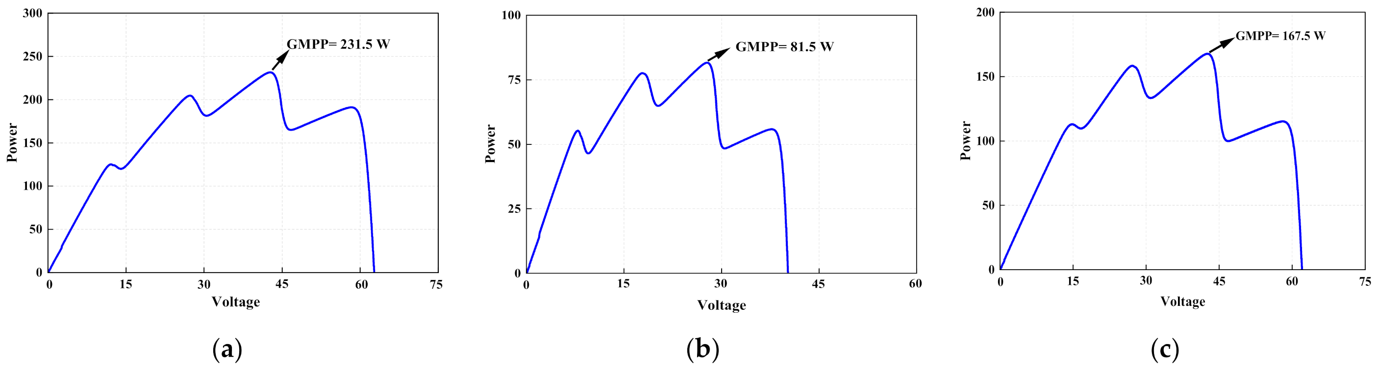
5.2. Partial Shading Conditions

To verify the potential of the proposed chimp-optimization-algorithm-based GMPPT technique under partial shading conditions, a comparative analysis with the most widely used modified P&O, PSO, FPA, and GWO-based MPPT methods was carried out. The irradiation profiles of the various non-uniform irradiation tests conducted to validate the performance of the proposed ChOA method under partial shading conditions are given in

Table 3. Irradiation profile.

Pattern\No	Row 1	Row 2	Row 3	Row 4
STC	1000 W/m2	1000 W/m2	1000 W/m2	1000 W/m2
UI-1	700 W/m2	700 W/m2	700 W/m2	700 W/m2
UI-2	500 W/m2	500 W/m2	500 W/m2	500 W/m2
PS-1	1000 W/m2	700 W/m2	500 W/m2	300 W/m2
PS-2	500 W/m2	300 W/m2	200 W/m2	100 W/m2
PS-3	800 W/m2	600 W/m2	400 W/m2	200 W/m2

. The PV curves of non-uniform irradiation cases are shown in Figure 14. The simulation results for three non-uniform irradiance conditions (i.e., partial shading-1 (PS-1), partial shading-2 (PS-2), and partial shading-3 (PS-3)) and their relative comparison with other MPPT methods is shown in Figure 15.

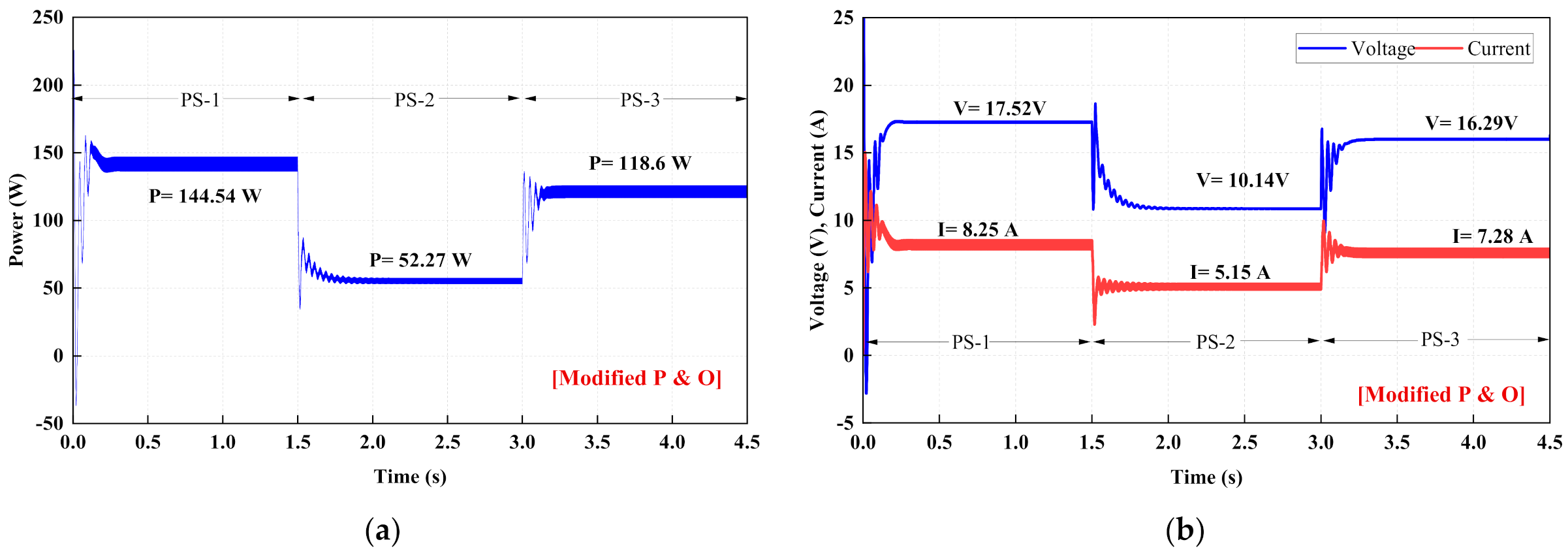
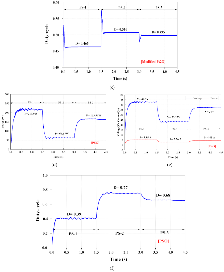
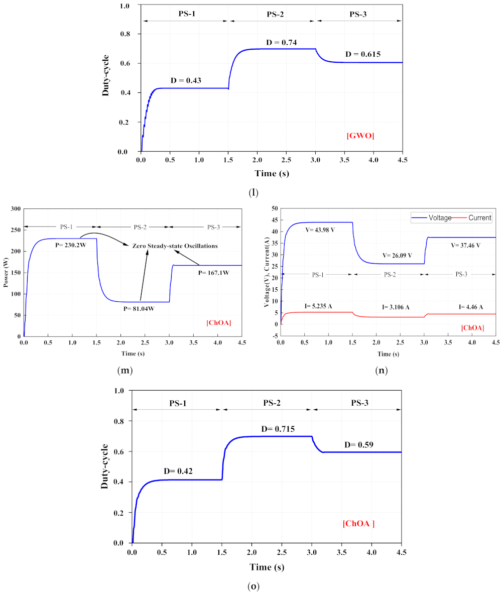
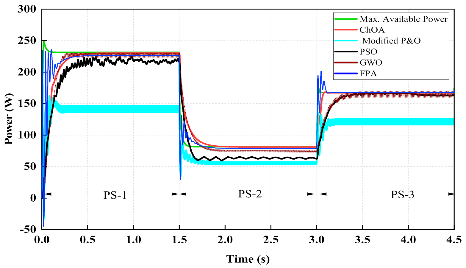
Comparative Analysis of Proposed ChOA with Modified P&O, PSO, FPA, and GWO Methods under Non-Uniform Irradiance Transition (PS-1→PS-2→PS-3)

The realization of simulation results is carried out using a PV array of 4 × 3 size in MATLAB Simulink software. In the case of non-uniform irradiance conditions, each row of the 4 × 3 PV array receives a different insolation level according to the irradiation patterns shown in Table 2. Initially, simulation is done considering a practical case of light and cloudy weather conditions, and the PV array is receiving an irradiance of PS-1 (1000, 700, 500, and 300 W/m²). In the case of these unequal irradiances on each row of PV array, the normalized voltage change goes beyond its threshold value, and as a result (according to the flowchart of Figure 5a and Equations (6) and (7)), the algorithm identifies the occurrence of non-uniform irradiance and calls the MPPT methods for GMPP tracking. As shown in Figure 15a, modified P&O tracks the MPP under non-uniform irradiance conditions and is stuck at a local optima of 144.54 W, having excessive initial and steady-state oscillations. PSO performs better and tracks a power of 219.9 W, as in Figure 15d. However, its tracking and steady-states have large oscillations, and as a result, PSO has power loss and is unable to track the exact MPP. The performance of FPA is superior as compared to previous methods, as it tracks a power of 229.6 W, as shown in Figure 15g, which is very close to an optimal power-point. Nonetheless, its high oscillatory tracking period causes power losses. The grey wolf optimization (GWO) approach reaches the power of 230 W, as evident in Figure 15j; however, its steady-state output is not stable. The continuous oscillating behavior causes efficiency problems.

On the other hand, the proposed ChOA tracks the GMPP at 230.2 W in just 0.5 s, having zero steady-state oscillations with an improved tracking efficiency of 99.43%, as visible in Figure 15m. The relative voltage and current characteristics are shown in Figure 15b,e,h,k,n, while duty-cycle waveforms are shown in Figure 15c,f,i,l,o.

At 1.5 s, a case of heavy clouds condition over PV array causes the transition of PS-1 to PS-2 (500, 300, 200, 100 W/m²). As a result, the operating point of the PV system is changed from a GMPP of 230.2 W to an unknown point. Again, the proposed detection method (flowchart in Figure 5a) differentiates it as non-uniform irradiance variation and reinitiates the MPPT algorithms for tracking GMPP. In this case, modified P&O is again unsuccessful in tracking the GMPP and is trapped at local MPP around 52.27 W with high initial and steady-state oscillations, as seen in Figure 15a. Although PSO has a better performance as compared to modified P&O, it is also trapped in the local maximum, tracking only power of 64.17 W. FPA and GWO settle at 78.63 W and 79.3 W, respectively. However, the proposed ChOA approach successfully tracks the new GMPP at 81.04 W, taking only 0.4 s of tracking time. The GMPP tracking efficiency in this case is also 99.43%. In addition, tracking duration has negligible oscillation, while steady-state condition when GMPP is tracked has zero oscillations, as evident in Figure 15m.

In the third case, the non-uniform irradiance changes from PS-2 to PS-3 (800, 600, 400, 200 W/m²) at 3 s. The proposed detection strategy successfully finds this change as non-uniform irradiance variation and retriggers the GMPP tracking methods. The modified P&O again fails and captures only power of 118.6 W. Contrarily, PSO tracks a power of 163.91 W, which is very close to the exact MPP of 167.5 W. However, PSO has unstable output, having oscillatory behavior around MPP, as evident in Figure 15d. The FPA and GWO methods have comparatively better performance and obtain a power of 164.1 W and 165.7 W. However, the oscillatory behavior of FPA during the tracking period and GWO during the steady-state period badly affects their efficiency. While the proposed chimp technique efficiently tracks the GMPP at 167.1 W with a minimum tracking time of 0.15 s and tracking efficiency of 99.76%, as shown in Figure 15m. Similar to the previous transition, the tracking duration has negligible oscillation, and the steady-state condition has the merit of zero oscillations. The output voltage and current characteristics of modified P&O, PSO, FPA, GWO, and ChOA under non-uniform irradiance transitions are shown in Figure 15b,e,h,k,n, while duty-cycle waveforms are shown in Figure 15c,f,i,l,o.

A comparison of different MPPT methods for tracking the maximum available power is demonstrated in Figure 16. The average MPPT tracking efficiency of modified P&O, PSO, FPA, GWO, and proposed ChOA methods is given in

Table 4. Performance comparison of various MPPT techniques.

MPPT Techniques	Max. Available Power	Tracked Power	Avg. Tracking Efficiency(%)
Modified P&O	PS-1 = 231.5 W, PS-2 = 81.5 W, PS-3 = 167.5 W	PS-1 = 144.54 W, PS-2 = 52.27 W, PS-3 = 118.6 W	65.78%
PSO	PS-1 = 231.5 W, PS-2 = 81.5 W, PS-3 = 167.5 W	PS-1 = 219.9 W, PS-2 = 64.17 W, PS-3 = 163.91 W	90.52%
FPA	PS-1 = 231.5 W, PS-2 = 81.5 W, PS-3 = 167.5 W	PS-1 = 229.6 W, PS-2 = 78.63 W, PS-3 = 164.1 W	97.87%
GWO	PS-1 = 231.5 W, PS-2 = 81.5 W, PS-3 = 167.5 W	PS-1 = 230 W, PS-2 = 79.3 W, PS-3 = 165.7 W	98.52%
ChOA	PS-1 = 231.5 W, PS-2 = 81.5 W, PS-3 = 167.5 W	PS-1 = 230.2 W, PS-2 = 81.04 W, PS-3 = 167.1 W	99.54%

. The comparative analysis of simulation results and MPP tracking efficiency confirms that the proposed chimp optimization algorithm (ChOA) technique has high efficiency, fast tracking time, and zero steady-state oscillations, outperforming all of the MPPT methods under study.

5.3. Load-Varying Conditions

To evaluate the robustness of the proposed ChOA method, a load variation test was conducted. Initially, the PV system is working smoothly at a GMPP of 230.2 W under the PS-1 case, with a resistive load of 8.4 Ω. At t = 1.5 s, the load is suddenly decreased to 4.5 Ω, and as a result, the output voltage is decreased, while current is increased, as evident in Figure 17. Based on Equation (5) and conditions explained in the flowchart of Figure 5a, the proposed chimp algorithm triggers by identifying this change as load variations and successfully tracks the GMPP of 230.2 W in just 0.25 s, as shown in the power characteristics of Figure 18.

At t = 3 s, the load is again changed from 4.5 Ω to 12 Ω, causing an increase in the voltage, while a decrease in current is visible in the output curves of Figure 17. Identical to the previous case, the proposed ChOA method detects this change as an increase in load and tracks back GMPP of 230.2 W at 3.35 s. Under both of the load-varying conditions, ChOA is efficiently tracking the GMPP with negligible tracking and steady-state fluctuations. Thus, results confirm the effectiveness of the proposed ChOA method against load variations.

6. Conclusions

The proposed hybrid MPPT techniques in this article determine the actual operating conditions of the PV system (i.e., uniform irradiance, non-uniform irradiance, and load-varying conditions). Based on the identified operating conditions, modified P&O or chimp optimization algorithms are used for MPPT tracking. To avoid simulation complexity and unnecessary computational burden, a modified P&O method is utilized to find MPP under uniformly changing irradiances. Modified P&O achieved an average steady-state MPPT efficiency of 96.92%, with a minimum possible tracking time of 0.4s. The deficiency of modified P&O under partial shading conditions is prevented by hybridizing it with a recently developed chimp-optimization-algorithm-based technique. The ChOA method successfully tackles the non-uniform irradiance and load-changing conditions. Using a group formation strategy, ChOA utilizes the excellent abilities of its groups to improve its overall performance. The proposed ChOA method has obtained an average MPPT efficiency of 99.54% with a minimum tracking time of 0.15s, as compared to 65.78%, 90.52%, 97.87%, and 98.52% efficiencies of modified P&O, PSO, FPA, and GWO, respectively, under non-uniform irradiance conditions. The robustness of the ChOA method is evident from the load variation test. Additionally, ChOA has negligible tracking oscillations and zero steady-state oscillations as compared to modified P&O, PSO, FPA, and GWO.

7. Future Work

Owing to the simplicity of operating conditions detection and ease of implementation, this technique has the benefit of easily embedding in existing PV plants. However, the identification of actual operating conditions and hybrid GMPP tracking technique proposed in this work is solely based on and verified using MATLAB simulations. In our future work, we have a plan to experimentally verify the performance of the proposed techniques in a real-time grid integration model. Moreover, there is a possibility of efficient control to enhance power network interoperability under high penetration of renewables by employing the proposed techniques.

References

1. Olowu, T.O.; Sundararajan, A.; Moghaddami, M.; Sarwat, A.I. Future challenges and mitigation methods for high photovoltaic penetration: A survey. Energies 2018, 11, 1782. [Google Scholar] [CrossRef] [Green Version]
2. Pendem, S.R.; Mikkili, S. Modelling and performance assessment of PV array topologies under partial shading conditions to mitigate the mismatching power losses. Sol. Energy 2018, 160, 303–321. [Google Scholar] [CrossRef]
3. Dhanalakshmi, B.; Rajasekar, N. A novel competence square based PV array reconfiguration technique for solar PV maximum power extraction. Energy Convers. Manag. 2018, 174, 897–912. [Google Scholar] [CrossRef]
4. Cherukuri, S.K.; Kumar, B.P.; Raj, K.K.; Muthubalaji, S.; Devadasu, G.; Babu, T.S.; Alhelou, H.H. A Novel Array Configuration Technique for Improving the Power Output of the Partial Shaded Photovoltaic System. IEEE Access 2022, 10, 15056–15067. [Google Scholar] [CrossRef]
5. Sharma, S.; Varshney, L.; Elavarasan, R.M.; Vardhan, A.S.; Vardhan, A.S.; Saket, R.K.; Subramaniam, U.; Hossain, E. Performance Enhancement of PV System Configurations Under Partial Shading Conditions Using MS Method. IEEE Access 2021, 9, 56630–56644. [Google Scholar] [CrossRef]
6. Jazayeri, M.; Uysal, S.; Jazayeri, K. A comparative study on different photovoltaic array topologies under partial shading conditions. In Proceedings of the 2014 IEEE PES T&D Conference and Exposition, Chicago, IL, USA, 14–17 April 2014; pp. 1–5. [Google Scholar]
7. Villalva, M.G.; Gazoli, J.R.; Filho, E.R. Comprehensive approach to modeling and simulation of photovoltaic arrays. IEEE Trans. Power Electron. 2009, 24, 1198–1208. [Google Scholar] [CrossRef]
8. Safari, A.; Mekhilef, S. Simulation and hardware implementation of incremental conductance MPPT with direct control method using cuk converter. IEEE Trans. Ind. Electron. 2010, 58, 1154–1161. [Google Scholar] [CrossRef]
9. Fapi, C.B.N.; Wira, P.; Kamta, M.; Badji, A.; Tchakounte, H. Real-time experimental assessment of Hill Climbing MPPT algorithm enhanced by estimating a duty cycle for PV system. Int. J. Renew. Energy Res. 2019, 9, 1180–1189. [Google Scholar]
10. Esram, T.; Kimball, J.W.; Krein, P.T.; Chapman, P.L.; Midya, P. Dynamic maximum power point tracking of photovoltaic arrays using ripple correlation control. IEEE Trans. Power Electron. 2006, 21, 1282–1291. [Google Scholar] [CrossRef]
11. Enslin, J.H.; Wolf, M.S.; Snyman, D.B.; Swiegers, W. Integrated photovoltaic maximum power point tracking converter. IEEE Trans. Ind. Electron. 1997, 44, 769–773. [Google Scholar] [CrossRef] [Green Version]
12. Sher, H.A.; Murtaza, A.F.; Noman, A.; Addoweesh, K.E.; Al-Haddad, K.; Chiaberge, M. A new sensorless hybrid MPPT algorithm based on fractional short-circuit current measurement and P&O MPPT. IEEE Trans. Sustain. Energy 2015, 6, 1426–1434. [Google Scholar]
13. Ahmed, J.; Salam, Z. A critical evaluation on maximum power point tracking methods for partial shading in PV systems. Renew. Sustain. Energy Rev. 2015, 47, 933–953. [Google Scholar] [CrossRef]
14. Gupta, A.K.; Pachauri, R.K.; Maity, T.; Chauhan, Y.K.; Mahela, O.P.; Khan, B.; Gupta, P.K. Effect of Various Incremental Conductance MPPT Methods on the Charging of Battery Load Feed by Solar Panel. IEEE Access 2021, 9, 90977–90988. [Google Scholar] [CrossRef]
15. Sundaram, B.M.; Manikandan, B.V.; Kumar, B.P.; Winston, D.P. Combination of novel converter topology and improved MPPT algorithm for harnessing maximum power from grid connected solar PV systems. J. Electr. Eng. Technol. 2019, 14, 733–746. [Google Scholar] [CrossRef]
16. Bhukya, M.N.; Kota, V.R.; Depuru, S.R.; Reddy, M.P.P.; Reddy, G.H. An Effective Design and Implementation of Hybrid MPP Tracking Scheme Based on Linear Tangents & Neville Interpolation (LT-NI) Technique for Photovoltaic (PV) System. IEEE Access 2021, 9, 68266–68276. [Google Scholar]
17. Houam, Y.; Terki, A.; Bouarroudj, N. An Efficient Metaheuristic Technique to Control the Maximum Power Point of a Partially Shaded Photovoltaic System Using Crow Search Algorithm (CSA). J. Electr. Eng. Technol. 2021, 16, 381–402. [Google Scholar] [CrossRef]
18. Pillai, D.S.; Ram, J.P.; Ghias, A.M.; Mahmud, M.A.; Rajasekar, N. An Accurate, Shade Detection-Based Hybrid Maximum Power Point Tracking Approach for PV Systems. IEEE Trans. Power Electron. 2019, 35, 6594–6608. [Google Scholar] [CrossRef]
19. Sundareswaran, K.; Peddapati, S.; Palani, S. MPPT of PV systems under partial shaded conditions through a colony of flashing fireflies. IEEE Trans. Energy Convers. 2014, 29, 463–472. [Google Scholar]
20. Hua, C.-C.; Zhan, Y.-J. A Hybrid Maximum Power Point Tracking Method without Oscillations in Steady-State for Photovoltaic Energy Systems. Energies 2021, 14, 5590. [Google Scholar] [CrossRef]
21. Ostadrahimi, A.; Mahmoud, Y. Novel Spline-MPPT Technique for Photovoltaic Systems under Uniform Irradiance and Partial Shading Conditions. IEEE Trans. Sustain. Energy 2020, 12, 524–532. [Google Scholar] [CrossRef]
22. Mobarak, M.H.; Bauman, J. A Fast Parabolic-Assumption Algorithm for Global MPPT of Photovoltaic Systems Under Partial Shading Conditions. IEEE Trans. Ind. Electron. 2021. [Google Scholar] [CrossRef]
23. Ahmed, J.; Salam, Z.; Kermadi, M.; Afrouzi, H.N.; Ashique, R.H. A skipping adaptive P&O MPPT for fast and efficient tracking under partial shading in PV arrays. Int. Trans. Electr. Energy Syst. 2021, 31, e13017. [Google Scholar]
24. Mohanty, S.; Subudhi, B.; Ray, P.K. A new MPPT design using grey wolf optimization technique for photovoltaic system under partial shading conditions. IEEE Trans. Sustain. Energy 2015, 7, 181–188. [Google Scholar] [CrossRef]
25. Deboucha, H.; Shams, I.; Belaid, S.L.; Mekhilef, S. A Fast GMPPT Scheme Based on Collaborative Swarm Algorithm for Partially Shaded photovoltaic system. IEEE J. Emerg. Sel. Top. Power Electron. 2021, 9, 5571–5580. [Google Scholar] [CrossRef]
26. Pervez, I.; Shams, I.; Mekhilef, S.; Sarwar, A.; Tariq, M.; Alamri, B. Most Valuable Player Algorithm Based Maximum Power Point Tracking for a Partially Shaded PV Generation System. IEEE Trans. Sustain. Energy 2021, 12, 1876–1890. [Google Scholar] [CrossRef]
27. Eltamaly, A.M.; Farh, H.M. Dynamic global maximum power point tracking of the PV systems under variant partial shading using hybrid GWO-FLC. Sol. Energy 2019, 177, 306–316. [Google Scholar] [CrossRef]
28. Kermadi, M.; Salam, Z.; Ahmed, J.; Berkouk, E.M. A high-performance global maximum power point tracker of PV system for rapidly changing partial shading conditions. IEEE Trans. Ind. Electron. 2020, 68, 2236–2245. [Google Scholar] [CrossRef]
29. Ali, E.M.; Abdelsalam, A.K.; Youssef, K.H.; Hossam-Eldin, A.A. An Enhanced Cuckoo Search Algorithm Fitting for Photovoltaic Systems’ Global Maximum Power Point Tracking under Partial Shading Conditions. Energies 2021, 14, 7210. [Google Scholar] [CrossRef]
30. Zhao, Z.; Cheng, R.; Yan, B.; Zhang, J.; Zhang, Z.; Zhang, M.; Lai, L.L. A dynamic particles MPPT method for photovoltaic systems under partial shading conditions. Energy Convers. Manag. 2020, 220, 113070. [Google Scholar] [CrossRef]
31. Singh, N.; Gupta, K.K.; Jain, S.K.; Dewangan, N.K.; Bhatnagar, P. A Flying Squirrel Search Optimization for abb: MPPT under Partial Shaded Photovoltaic System. IEEE J. Emerg. Sel. Top. Power Electron. 2020, 9, 4963–4978. [Google Scholar] [CrossRef]
32. Khishe, M.; Mosavi, M.R. Chimp optimization algorithm. Expert Syst. Appl. 2020, 149, 113338. [Google Scholar] [CrossRef]
33. Yousri, D.; Thanikanti, S.B.; Balasubramanian, K.; Osama, A.; Fathy, A. Multi-objective grey wolf optimizer for optimal design of switching matrix for shaded PV array dynamic reconfiguration. IEEE Access 2020, 8, 159931–159946. [Google Scholar] [CrossRef]
34. Varshney, S.K.; Khan, Z.A.; Husain, M.A.; Tariq, A. A comparative study and investigation of different diode models incorporating the partial shading effects. In Proceedings of the 2016 International Conference on Electrical, Electronics, and Optimization Techniques (ICEEOT), Chennai, India, 3–5 March 2016; pp. 3145–3150. [Google Scholar]
35. Tey, K.S.; Mekhilef, S.; Seyedmahmoudian, M.; Horan, B.; Oo, A.T.; Stojcevski, A. Improved differential evolution-based MPPT algorithm using SEPIC for PV systems under partial shading conditions and load variation. IEEE Trans. Ind. Inform. 2018, 14, 4322–4333. [Google Scholar] [CrossRef]
Figure 1. Equivalent circuit of single diode model.
Energies 15 01549 g001
Figure 2. I-V curve during uniform irradiance change and partial shading.
Energies 15 01549 g002
Figure 3. I-V curve’s response to load variations.
Energies 15 01549 g003
Figure 4. I–V characteristics under combined variation of load and irradiance.
Energies 15 01549 g004
Figure 5. (a). Flowchart for identification of operating conditions. (b) Flowchart of the modified perturb and observe algorithm. (c) Flowchart of the chimp optimization algorithm.
Energies 15 01549 g005aEnergies 15 01549 g005bEnergies 15 01549 g005c
Figure 6. Schematic of proposed MPPT model.
Energies 15 01549 g006
Figure 7. (a). High oscillations power characteristics at STC. (b) Low oscillations power characteristics at STC.
Energies 15 01549 g007
Figure 8. High and low oscillations V-I characteristics at STC.
Energies 15 01549 g008
Figure 9. PV Curves of uniform irradiance cases: (a) STC (1000 W/m2), (b) UI-1 (700 W/m2), (c) UI-2 (500 W/m2).
Energies 15 01549 g009
Figure 10. Power characteristics during irradiance transition (STC→UI-1), (a) high oscillations, and (b) low oscillations.
Energies 15 01549 g010
Figure 11. High and low oscillations V-I characteristics during irradiance transition (STC→UI-1).
Energies 15 01549 g011
Figure 12. Power characteristics during irradiance transition (UI-1→UI-2): (a) high oscillations, (b) low oscillations.
Energies 15 01549 g012
Figure 13. High and low oscillations V-I characteristics during irradiance transition (UI-1→UI-2).
Energies 15 01549 g013
Figure 14. PV curves of non-uniform irradiance cases (a) PS-1, (b) PS-2, and (c) PS-3.
Energies 15 01549 g014
Figure 15. GMPP tracking profile of modified P&O, PSO, FPA, GWO, and proposed ChOA under non-uniform irradiance variations: (a,d,g,j,m) power characteristics, (b,e,h,k,n) voltage and current characteristics, (c,f,i,l,o) duty-cycle characteristics.
Energies 15 01549 g015aEnergies 15 01549 g015bEnergies 15 01549 g015cEnergies 15 01549 g015d
Figure 16. GMPP tracking performance of different MPPT methods.
Energies 15 01549 g016
Figure 17. V-I characteristics during load variations.
Energies 15 01549 g017
Figure 18. Power characteristics during load variation.
Energies 15 01549 g018