Abstract
In this paper, an attempt at the energy optimization of perfect control systems is performed. The perfect control law is the maximum-speed and maximum-accuracy procedure, which allows us to obtain a reference value on the plant’s output just after a time delay. Based on the continuous-time state-space description, the minimum-error strategy is discussed in the context of possible solutions aiming for the minimization of the control energy. The approach presented within this study is focused on the nonunique matrix inverse-originated so-called degrees of freedom being the core of perfect control scenarios. Thus, in order to obtain the desired energy-saving parameters, a genetic algorithm has been employed during the inverse model control synthesis process. Now, the innovative continuous-time procedure can be applied to a wide range of multivariable plants without any stress caused by technological limitations. Simulation examples made in the MATLAB/Simulink environment have proven the usefulness of the new method shown within the paper. In the extreme case, the energy consumption has been reduced by approximately 80% in comparison with the well-known Moore–Penrose inverse.
1. Introduction
The widely understood energy optimization is an important subject gathering worldwide scientific research interest. Energy efficiency of cars, buildings and electronic devices plays an essential role in limiting CO production, providing a wide area for possible development [1,2]. Energy-saving appliances, together with a widely understood sustainability, is currently a very popular and actual topic due to climate changes. With both technological and social changes, the main goal is to limit the pollution generated by humankind [3]. Naturally, the main part of the interest is focused on declining fossil fuels to be replaced with environment-friendly sources of energy [4,5]. On the other hand, the already produced energy should be used as effectively as possible, minimizing both energy losses and consumption. It is worth mentioning that a small reduction in power demand in a single appliance can result in significant, world-wide energy saving [6]. Of course, the changes can be obtained in both hardware and software fields as these two aspects are impossible to separate in modern solutions.
One of the key areas where energy efficiency is crucial is hybrid and electric vehicles, affecting their range and overall serviceableness [7]. Moreover, some specific methods of energy recovery and distribution have been developed, allowing us to significantly lower the demand on power [8,9,10,11]. Nevertheless, aside from mentioned solutions, there are plenty of applications where the software plays a crucial role. A properly developed control system, e.g., for a gearshift, can enhance the power management for a hybrid V6 unit [12]. Therefore, the optimization of control algorithms and software is of major importance here.
For years, different studies were aiming for the possible energy minimization of various control algorithms. The practical aspects of this issue are obvious, concerning the already mentioned applications. On the other hand, there are theoretical papers usually dealing with problems derived from specified system descriptions. For instance, an algorithm allowing to shift the state variables to desired values along with the analytically proven minimum-energy trajectory has been derived from plants described in the state-space framework [13]. Of course, the energy-based study can be performed in a less formal way, where the goal function is declared and minimized using different methods of a control design process. The energy demand can be anticipated during the control synthesis itself. For example, in the Linear-Quadratic (LQ) or Linear-Quadratic-Gaussian (LQG) regulation, the control energy is strictly influenced by the weighting matrix parameters associated with the target function, which are finally used for solving the Riccatti equation in the proper context [14,15]. It is worth mentioning that the fuzzy control algorithm can also be subjected to the discussed energy-oriented optimization [16].
Naturally, the usual compromise between control energy and control speed or control error is the main issue here. It is self-explanatory that a more accurate and faster control scenario will demand more energy consumption to meet the imposed requirements. Some algorithms are strictly based on the examined consensus, to mention LQ regulation that is formulated in regard to the specified performance function. However, there are also some control scenarios, which are invulnerable in terms of energy-error compromise. For example, the perfect control algorithm maintains its minimum-error property under different energy intakes [17]. This feature, however, excels for multivariable, in particular, nonsquare, systems [18].
The perfect control algorithm gathers an increasing scientific interest due to its minimum-error behavior. For now, for discrete-time state-space plants, it has been shown that the inverse-based perfect control scheme can be enhanced in different manners [19]. Features such as robustness or higher speed were assigned to the closed-loop systems using the well-known state-feedback approach. Of course, such peculiarities are available only for nonsquare systems, where there are an infinite number of possible input combinations resulting in the same output behavior [20].
Model inversion drew attention in many fields from security to control [21]. In the multivariable inverse model control, such as the perfect control, the sets of equivalent instances can be obtained using nonunique matrix inverses. Henceforth, there is a need to distinguish between ‘good’ and ‘bad’ solutions. Of course, the commonly used unique Moore–Penrose inverse can provide here a useful benchmark in order to assess the properties connected with a particular result [22,23]. On the other hand, the nonunique inverses usually contain the so-called degrees of freedom, which allow us to obtain the already mentioned numerous perfect control solutions. What is worth mentioning is that the different inverses have different forms connected with a plethora of degrees of freedom; therefore, some inverses may be preferable in specific applications [24]. In all available instances and inverses, the perfect control, however, predefines the perfect output property. It is also worth pointing out that, in the case of classical one-delayed discrete-time systems, the output is driven to the reference value in a single step, while for continuous-time plants the similar behavior is obtained in regard to specified solver time, minimizing the control error [17,20]. So, the said perfectness for both discrete- and continuous-time processes should be understood in the terms of possible minimum control error to be achieved.
Since the output behavior is guaranteed for all perfect control systems, the research challenge is now to find such nonunique inverses that will fulfill the imposed constrains. The obvious methods for searching the solution minimizing the attained goal function are the directional or gradient optimization approaches [25,26]. The other way of finding the optimal values for a given problem is the linear programming. This method has successfully been used for, e.g., optimization of unit commitment and economic dispatch in microgrids [27,28] or virtual network functions placement as well as routing problems [29]. Since the considered control strategy is obtained for linear dynamic systems for now, the approach covering linear programming may be successful here, assuming the goal function is of valid form. Notwithstanding, the usage of methods based on the genetic algorithm paradigm seems to be more interesting in terms of the multivariable nonsquare optimization problem [7,30].
Genetic algorithm has been used for decades now in order to obtain new solutions for well-established issues [31,32,33]. Based on Darwin’s Theory, whole mathematical machinery can be formulated and applied in both practical and analytical manners. In such algorithms, the process of natural selection is imitated, so the fittest units are selected to pass their characteristics to the next generations. At the beginning, there is a need to specify the starting/initial population, which constitutes the basis of available features. Later, based on the so-called fitness function, the specified individuals are selected to share their genes with future algorithm iterations. Naturally, the mutations are also taken into consideration, allowing new properties to emerge within the population [34]. With such behavior, the genetic algorithms are widely used in modern science and engineering. Of course, in this paper, a genetic algorithm will be used to minimize the energy observed during the control scheme performed for a selected plant.
Therefore, aiming for the energy-based optimization of continuous-time perfect control systems, the remainder of this paper is organized as follows. At the beginning, the mathematical preliminaries are described in order to bring closer the idea of a perfect control algorithm and nonsquare matrix inverses. The analytical formulation of the optimization problem is given in Section 3. Simulation examples covering the application of genetic algorithm in the MATLAB/Simulink environment (The MathWorks, Inc., Natick, MA, USA) are given in Section 4. Section 5 constitutes a short brief of open problems, which are still waiting to be solved in the context given within this paper. In the end, the closing remarks are given in the ultimate section of the manuscript.
2. Preliminaries
The perfect control algorithm is based on a model of the particular process; thus, the mathematical description of dynamics is crucial here. In this paper, we are considering the well-known continuous-time state-space representation. This framework consists of the state equation as follows
where is the system matrix, is the input matrix, whereas and are the n-state and -control vectors, respectively. The output of system, with initial condition , is obtained in accordance with the following formula
where is the output matrix and constitutes the -output signal. For such state-space plants, some properties have analytically been established, e.g., the stability of the state-space model is connected with eigenvalues of the system matrix with the following relationship
from which it is clear that the object is stable if all of its poles are located within the left half of the open complex plane. Now, taking into account the equation describing the dependency between two values of the function defined in the continuous-time domain [20]
a specified solver can be arranged in order to obtain the simulation later. Naturally, in such a case, the Euler-based differential solver is taken into consideration. For a system described in the mentioned framework, the perfect control algorithm is obtained in regard to the output behavior, which can be described as follows
As it has been shown in Reference [20], the perfect control law for continuous-time state-space systems can be defined in the following manner
where matrix sounds as
whilst and stand for any right and left generalized inverse, respectively. In the case of right-invertible plants, the most important relation considering right matrix inverses is expressed
which allow us, e.g., to obtain the zero steady-state error in the inverse model control scenarios. Moreover, it is worth mentioning that for zero reference values, the control Equation (6) reduces to the following form
In the approach concerning nonsquare matrices, the inverse is however nonunique; thus, the only one from a plethora of solutions may be chosen. For all proper right inverses applied in the considered study, the perfectness of control strategy is presumed. After substitution of the control and state equation into the output formula, the following outcome is observed
Remark 1.
Interestingly, the above presented MIMO approach can be adjusted to a MISO plant, since the previously given matrix of Equation (7) can be reduced to the following form
where m is expressed by
The proposed simplified form of the discussed matrix from Equation (11) can easily be verified in the continuous-time perfect control-originated way
Therefore, the desired output behavior is obtained in both MIMO and MISO scenarios. It will especially be useful when dealing with simple cases, where the computational burden will be significantly eased.
With such a closed-loop control system design, the output stability is guaranteed with its nonzero derivative present only for the nonzero control error. As soon as the control error disappears, the steady state is obtained with zero energy input (for the zero-reference value). The transient output state, however, lasts for a single calculation step, during which the exact amount of energy is injected into the system to reach the output setpoint. All non-Dirac-oriented control signals are used only for plant dynamics compensation. Thereby, an attempt for the energy optimization is made in the next crucial section.
3. Problem Formulation
As it is highlighted in the previous section, during the perfect control design, there is a possibility to apply the nonunique matrix inverses. As there is plenty (or even an infinite number of) possible solutions, the challenge is to address the potential advantages derived from the different types of inverses. In this particular study, the aim is to minimize the control energy, so the goal function can be declared as
where is the final simulation time. Of course, this parameter should be set properly in order to take into consideration all of the transient states and energy intake of the control scenario. It has been shown in the past that the control energy can be influenced with a selection of the nonunique matrix inverse, which constitutes a core part of the state feedback consideration. In this examination, the right -inverse in the following form [17]
where involves the so-called degrees of freedom, was taken to enable the energy optimization task.
Remark 2.
In the case of we arrive at minimum norm T-inverse in the subsequent form
which has been used for decades in different theoretical and practical implementations. Notwithstanding, it has also been shown that solutions other than the minimum norm one can outperform the classical approach to the matrix inverse problem. Of course, the unique solution does not ensure any possibility to improve the energy performance.
Therefore, in this particular study, an attempt at energy minimization will be performed based on the following control formula
obtained by joining Equations (6) and (15). Here, the degree of freedom is in a direct form, so it can be a parameter in the proper energy-based optimization. Of course, due to enabling the proper optimization process, the performance index needs to be clearly specified. Hence, the final target of this study is to find the optimal value according to the expressed performance index
Remark 3.
In this particular paper, we assume that β is a parameter matrix. It would be interesting to apply the degree of freedom involving polynomial inside. It has been shown that the polynomial degrees of freedom can be useful in the inverse-based operations. For now, however, the mentioned framework should be treated as an open problem worth further intense investigation.
The crucial energy-based examinations will be supported using the standard MATLAB-type genetic algorithm, which is implemented within the optimization toolbox. Since the genetic algorithm is only a tool in this study, the main concern will be put around its application devoted to the minimum energy-related continuous-time perfect control design. Therefore, let us now continue with the simulation examples covering three different cases of the multivariable perfect control systems optimization.
4. Simulation Examples
In this section, the representative three numerical examples will be given in order to confirm the proper operation of the control law together with its energy optimization. All the simulations were carried out in the MATLAB/Simulink environment using the (Euler) solver with the fixed time step equal to = 0.001 s. Selection of the accurate step of time is crucial here, as according to Equations (6) and (7) it influences the control properties. Naturally, it can also be of variable size; however, such a scenario requires more calculation efforts to perform control actions. Moreover, plants with different complexity were selected to check the applicability of the proposed new approach.
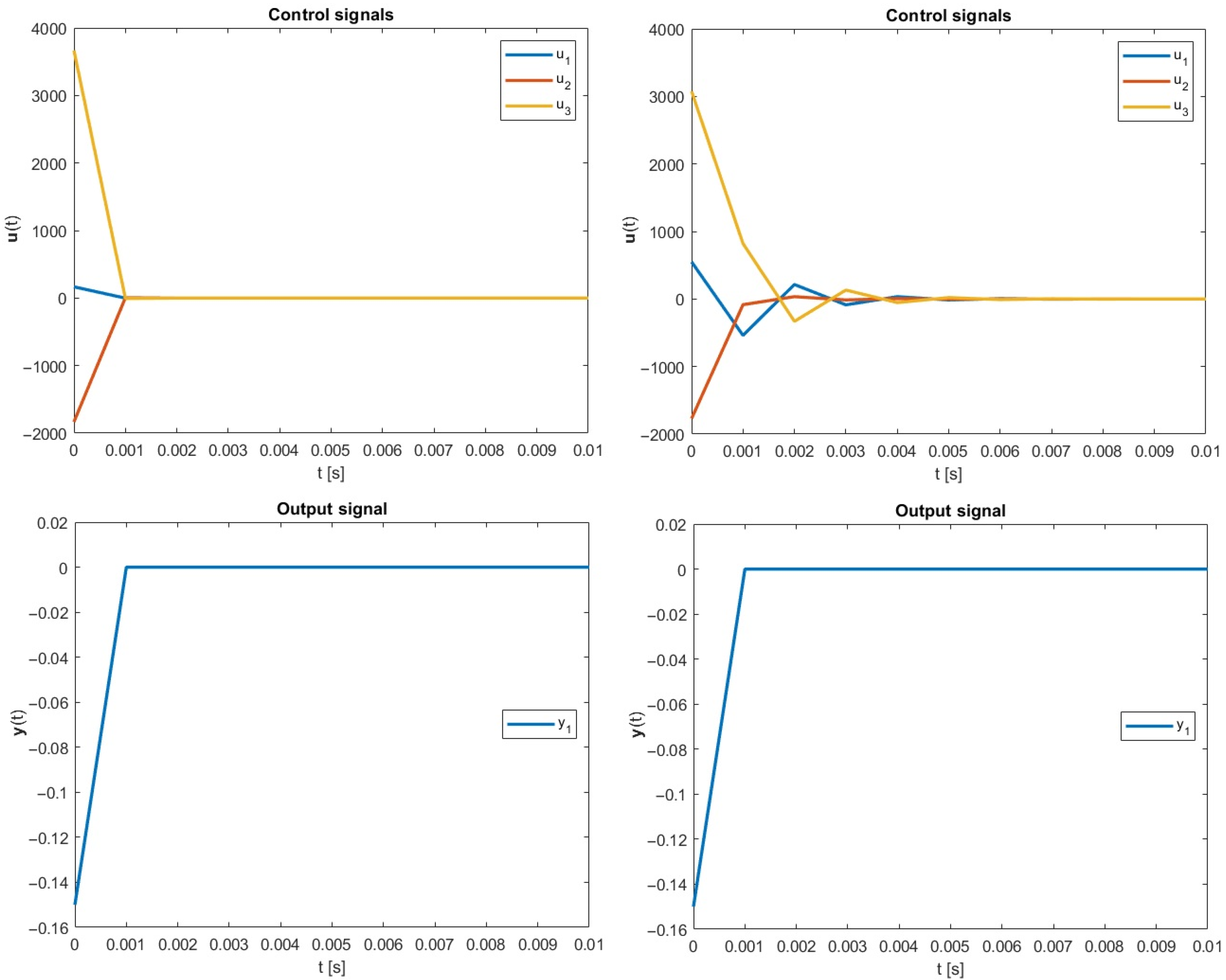
4.1. Three-by-One Unstable System
As a first example, we are considering the continuous-time plant with three inputs, three state variables and one output, defined through the following matrices
having the initial condition . It is worth mentioning that the system poles were equal to . Due to the fact that the considered system has only one output, it is correct to use the simplified form of the perfect control law determined by Equations (11) and (12) for the entire simulation process. With the use of a genetic algorithm, the attempt to minimize the control energy was made by searching for such a degree of freedom , which will result in the lowest value of the performance index (14) or rather the norm (18).
Starting the optimization from the minimum-norm right T-inverse, the genetic algorithm with a number of iterations had returned the degree of freedom as below
which was applied to the perfect control design strategy. The resulting control and output signals, for both minimum norm and the optimal degree of freedom, are presented in Figure 1. It is worth emphasizing that the values of the performance index were equal to for the minimum-norm approach and after the optimization process. Thus, the energy demand to execute the control scenario was reduced here by approximately .
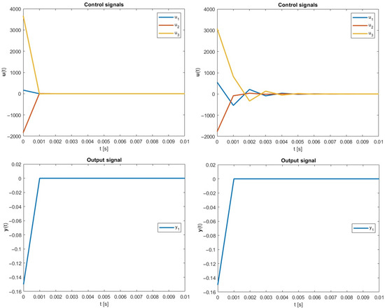
Figure 1.
Simulation results, case 1: (left) the Moore–Penrose approach; (right) the new energy-optimal approach; .
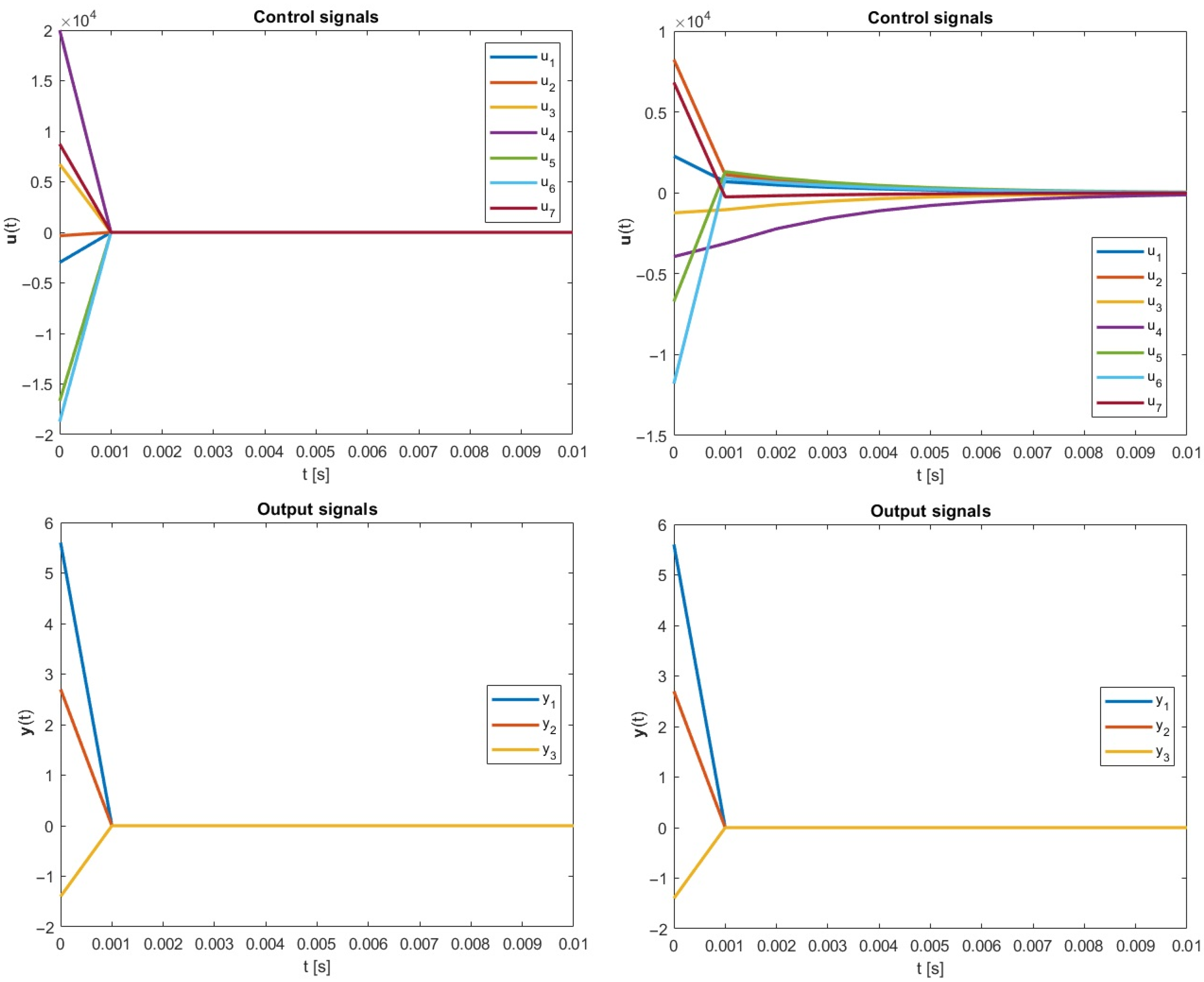
4.2. Seven-by-Three Unstable System
Another example employs a more complicated, unstable system with multiple input and output variables, governed by the following matrices
being under the initial condition . In this scenario, where , the usage of the genetic algorithm had returned the subsequent optimal degree of freedom
As before, better results, in the context of energy consumption, were received using the new framework. The plots of the control and output signals of both approaches are shown below in Figure 2.
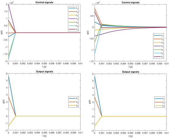
Figure 2.
Simulation results, case 2: (left) Moore–Penrose approach; (right) the new optimal energy approach; .
Even though the steady state of the control signals was obtained faster in the classical approach, the resulting total control energy was higher () than after the optimization process, where the final energy was equal to . In this scenario, the energy saving was remarkably close to .
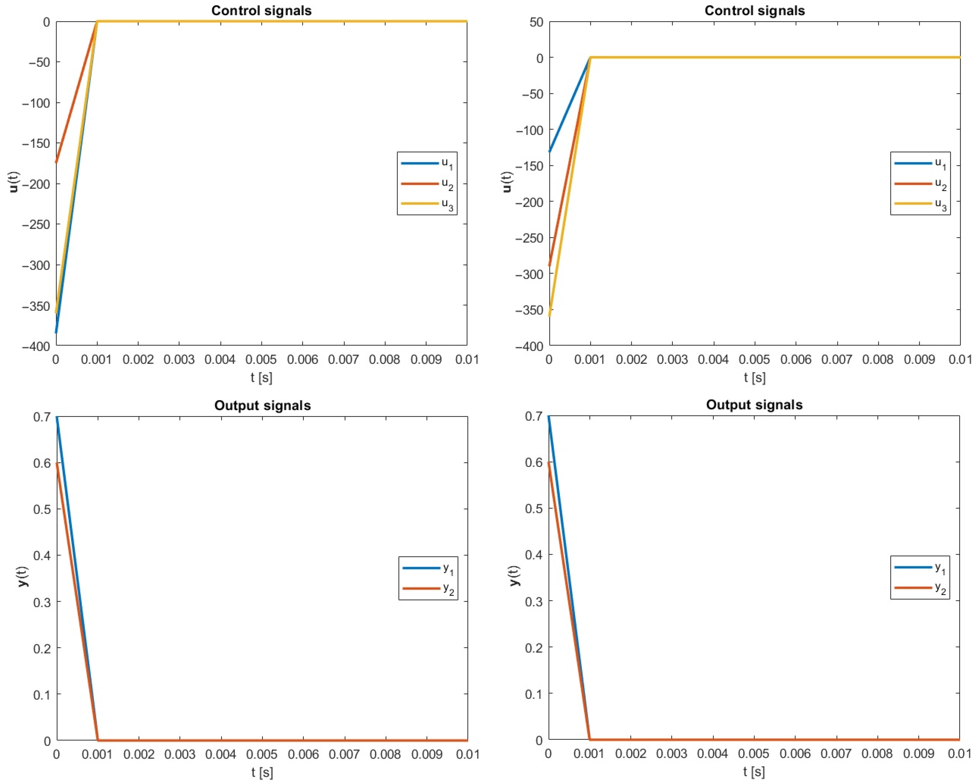
4.3. Cartesian Coordinate Robot
As an ultimate example, a Cartesian robot with the structure depicted in Figure 3 was subjected to the perfect control energy optimization task.
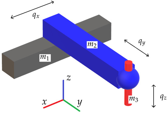
Figure 3.
Cartesian robot visualization.
The dynamic equations of the mentioned system were determined by the Euler–Lagrange method and can be written as follows [20]
where , , and . The state-space framework representation of the discussed object can be formed in the subsequent manner
The output equation can now be expressed as
The above assumption concerning the system output allows us to receive a resultant value of the movement speed in the XY-plane and velocity in the Z-axis. Now, for a known set of model parameters, in this case equal to , , , , and , the matrices of the state-space description have obtained the following values
To fully describe the considered plant, the initial condition was also defined. For such a system, the genetic-oriented procedure was conducted in order to obtain the optimal degree of freedom, which here was equal to
The simulations were carried out to again compare the minimum norm and optimized -inverse in the terms of energy consumption. The resulting plots are presented in Figure 4.
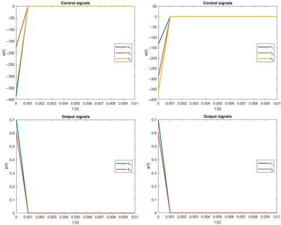
Figure 4.
Simulation results, case 3: (left): Moore–Penrose approach; (right): the new optimal energy approach; .
In this example, for the classical approach, the final control energy was equal to , while the optimization brought us the lower control cost which equals . In this scenario, the energy was reduced by around .
4.4. Discussion
As it can be seen in Table 1, in every considered simulation instance, the strategy based on the optimized -inverse is better than after the employment of the classical Moore–Penrose-related formula. Furthermore, results in output signals are the same for both methodologies. Thus, the new optimal energy control paradigm can be a good counterpart to this based on the obligatory well-known classical approach.

Table 1.
Comparison of simulation results provided by two methods.
Summing up, after the three simulation examples, we can state that the energy optimization process has successfully been applied to the continuous-time perfect control algorithm.
5. Open Problems
Dealing with a scenario such as perfect control algorithm, it very often provokes further questions than have been answered within a single paper. Therefore, some open problems are described in this section.
In this particular study, the right -inverse was used in the minimum-energy pursuit. As a number of other inverses are available, just to mention the H- or S-inverse, there are still possibilities to further enhance the perfect control design.
Moreover, it has been highlighted that the usage of polynomial degrees of freedom (even in the inverses of parameter matrices) can benefit the design of perfect control schemes, only for discrete-time systems for now. Therefore, it is still needed to investigate how the mentioned polynomial degrees of freedom will affect the perfect control scenarios for continuous-time plants.
In this paper, the zero-referenced value systems are taken into consideration in the energy optimization problem. For nonzero setpoint, however, we expect some more complex closed-loop behavior, deriving from nonzero steady states of both control and state variables. Hence, an additional optimization should be undertaken in order not only to minimize the transient control energy but also to find such state and reference gain to finally obtain the possible low energy consumption under the constant output behavior. Supplementary studies should also be conducted in the terms of application of other MATLAB-related solvers.
Summing up, with the recent disclosure of the perfect control algorithm for continuous-time plants, a very new research branch appeared. More studies concerning the energy optimization, robustification or pole-placement method of the continuous-time perfect control strategy shall be performed in the nearest future.
6. Summary
In this paper, the energy-related optimization problem of the perfect control systems is performed using genetic algorithm. Based on the goal function, the discussed total control energy is minimized with a proper selection of the inverse matrix used in the perfect state-feedback gain. The usage of different degrees of freedom resulted in measurable benefits, which are now possible to apply to both discrete- and continuous-time plants involving the real-life practical ones. The reduction in the energy effort has been around 80% against the application of the classical Moore–Penrose inverse.
Author Contributions
Conceptualization, W.P.H., M.K., P.M. and T.F.; methodology, W.P.H., M.K., P.M. and T.F.; software, P.M. and M.K.; validation, W.P.H., M.K., P.M. and T.F.; formal analysis, W.P.H. and T.F.; investigation, W.P.H., M.K., P.M. and T.F.; resources, M.K. and P.M.; data curation, P.M. and M.K.; writing—original draft preparation, M.K., W.P.H. and P.M.; writing—review and editing, M.K. and P.M.; visualization, W.P.H., M.K. and P.M.; supervision, W.P.H.; project administration, W.P.H. All authors have read and agreed to the published version of the manuscript.
Funding
This research received no external funding.
Institutional Review Board Statement
Not applicable.
Informed Consent Statement
Not applicable.
Data Availability Statement
Data are contained within the article.
Conflicts of Interest
The authors declare no conflict of interest.
References
- Kovacic, I.; Reisinger, J.; Honic, M. Life Cycle Assessment of embodied and operational energy for a passive housing block in Austria. Renew. Sustain. Energy Rev. 2018, 82, 1774–1786. [Google Scholar] [CrossRef]
- Jareemit, D.; Limmeechokchai, B. Influence of Changing Behavior and High Efficient Appliances on Household Energy Consumption in Thailand. Energy Procedia 2017, 138, 241–246. [Google Scholar] [CrossRef]
- George, G.; Merrill, R.K.; Schillebeeckx, S.J.D. Digital Sustainability and Entrepreneurship: How Digital Innovations Are Helping Tackle Climate Change and Sustainable Development. Entrep. Theory Pract. 2021, 45, 999–1027. [Google Scholar] [CrossRef] [Green Version]
- Brockway, P.E.; Owen, A.; Brand-Correa, L.I.; Hardt, L. Estimation of global final-stage energy-return-on-investment for fossil fuels with comparison to renewable energy sources. Nat. Energy 2019, 4, 612–621. [Google Scholar] [CrossRef] [Green Version]
- Perez-Villalpando, M.A.; Gurubel Tun, K.J.; Arellano-Muro, C.A.; Fausto, F. Inverse Optimal Control Using Metaheuristics of Hydropower Plant Model via Forecasting Based on the Feature Engineering. Energies 2021, 14, 7356. [Google Scholar] [CrossRef]
- Danish, M.S.S.; Bhattacharya, A.; Stepanova, D.; Mikhaylov, A.; Grilli, M.L.; Khosravy, M.; Senjyu, T. A Systematic Review of Metal Oxide Applications for Energy and Environmental Sustainability. Metals 2020, 10, 1604. [Google Scholar] [CrossRef]
- Lü, X.; Wu, Y.; Lian, J.; Zhang, Y.; Chen, C.; Wang, P.; Meng, L. Energy management of hybrid electric vehicles: A review of energy optimization of fuel cell hybrid power system based on genetic algorithm. Energy Convers. Manag. 2020, 205, 112474. [Google Scholar] [CrossRef]
- Arenas Urrea, S.; Díaz Reyes, F.; Peñate Suárez, B.; de la Fuente Bencomo, J.A. Technical review, evaluation and efficiency of energy recovery devices installed in the Canary Islands desalination plants. Desalination 2019, 450, 54–63. [Google Scholar] [CrossRef]
- Hussain, S.; Ahmed, M.A.; Kim, Y.-C. Efficient power management algorithm based on fuzzy logic inference for electric vehicles parking lot. IEEE Access 2019, 7, 65467–65485. [Google Scholar] [CrossRef]
- Hussain, S.; Kim, Y.-S.; Thakur, S.; Breslin, J.G. Optimization of Waiting Time for Electric Vehicles Using a Fuzzy Inference System. IEEE Trans. Intell. Transp. Syst. 2022, 1–12. [Google Scholar] [CrossRef]
- Hussain, S.; Ahmed, M.A.; Lee, K.-B.; Kim, Y.-C. Fuzzy logic weight based charging scheme for optimal distribution of charging power among electric vehicles in a parking lot. Energies 2020, 13, 3119. [Google Scholar] [CrossRef]
- Duhr, P.; Christodoulou, G.; Balerna, C.; Salazar, M.; Cerofolini, A.; Onder, C.H. Time-optimal gearshift and energy management strategies for a hybrid electric race car. Appl. Energy 2021, 282, 115980. [Google Scholar] [CrossRef]
- Klamka, J. Controllability and Minimum Energy Control of Linear Finite Dimensional Systems. In Controllability and Minimum Energy Control; Springer International Publishing: Cham, Switzerland, 2019; pp. 13–25. [Google Scholar] [CrossRef]
- Neacşu, D.O.; Sîrbu, A. Design of a LQR-Based Boost Converter Controller for Energy Savings. IEEE Trans. Ind. Electron. 2020, 67, 5379–5388. [Google Scholar] [CrossRef]
- Lee, K.; Jeon, S.; Kim, H.; Kum, D. Optimal Path Tracking Control of Autonomous Vehicle: Adaptive Full-State Linear Quadratic Gaussian (LQG) Control. IEEE Access 2019, 7, 109120–109133. [Google Scholar] [CrossRef]
- Maghfiroh, H.; Hermanu, C.; Ibrahim, M.H.; Anwar, M.; Ramelan, A. Hybrid fuzzy-PID like optimal control to reduce energy consumption. Telkomnika 2020, 18, 2053–2061. [Google Scholar] [CrossRef]
- Krok, M.; Hunek, W.P. Pole-Free vs. Minimum-Norm Right Inverse in Design of Minimum-Energy Perfect Control for Nonsquare State-Space Systems. In Biomedical Engineering and Neuroscience, Proceedings of the 3rd International Scientific Conference on Brain-Computer Interfaces, BCI 2018, Opole, Poland, 13–14 March 2018; Advances in Intelligent Systems and Computing; Springer: Cham, Switzerland, 2017; pp. 184–194. [Google Scholar] [CrossRef]
- Krok, M.; Hunek, W.P. Deadbeat vs. pole-free perfect control. In Proceedings of the 6th International Conference on Control, Decision and Information Technologies (CoDIT’19), Paris, France, 23–26 April 2019; pp. 1338–1343. [Google Scholar] [CrossRef]
- Hunek, W.P.; Krok, M. A study on a new criterion for minimum-energy perfect control in the state-space framework. Proc. Inst. Mech. Eng. Part I J. Syst. Control. Eng. 2019, 233, 779–787. [Google Scholar] [CrossRef]
- Majewski, P.; Hunek, W.P.; Krok, M. Perfect Control for Continuous-Time LTI State-Space Systems: The Nonzero Reference Case Study. IEEE Access 2021, 9, 82848–82856. [Google Scholar] [CrossRef]
- Khosravy, M.; Nakamura, K.; Hirose, Y.; Nitta, N.; Babaguchi, N. Model Inversion Attack by Integration of Deep Generative Models: Privacy-Sensitive Face Generation from a Face Recognition System. IEEE Trans. Inf. Forensics Secur. 2022, 17, 357–372. [Google Scholar] [CrossRef]
- Ben-Israel, A.; Greville, T.N.E. Generalized Inverses, Theory and Applications, 2nd ed.; Springer: New York, NY, USA, 2003. [Google Scholar]
- Kafetzis, I.S.; Karampetakis, N.P. On the algebraic structure of the Moore–Penrose inverse of a polynomial matrix. IMA J. Math. Control. Inf. 2021, dnab001. [Google Scholar] [CrossRef]
- Noueili, L.; Chagra, W.; Ksouri, M. New Iterative Learning Control Algorithm Using Learning Gain Based on σ Inversion for Nonsquare Multi-Input Multi-Output Systems. Model. Simul. Eng. 2018, 2018, 4195938. [Google Scholar] [CrossRef] [Green Version]
- Feng, Z.; Ma, N.; Li, W.; Narasaki, K.; Lu, F. Efficient analysis of welding thermal conduction using the Newton–Raphson method, implicit method, and their combination. Int. J. Adv. Manuf. Technol. 2020, 111, 1929–1940. [Google Scholar] [CrossRef]
- Kim, H.S.; Lim, Y.J.; Lee, H.L. Optimum location of outrigger in tall buildings using finite element analysis and gradient-based optimization method. J. Build. Eng. 2020, 31, 101379. [Google Scholar] [CrossRef]
- Nemati, M.; Braun, M.; Tenbohlen, S. Optimization of unit commitment and economic dispatch in microgrids based on genetic algorithm and mixed integer linear programming. Appl. Energy 2018, 210, 944–963. [Google Scholar] [CrossRef]
- Zhu, Z.; Tang, J.; Lambotharan, S.; Chin, W.H.; Fan, Z. An integer linear programming based optimization for home demand-side management in smart grid. In Proceedings of the 2012 IEEE PES Innovative Smart Grid Technologies (ISGT), Washington, DC, USA, 16–20 January 2012; pp. 1–5. [Google Scholar] [CrossRef]
- Addis, B.; Belabed, D.; Bouet, M.; Secci, S. Virtual network functions placement and routing optimization. In Proceedings of the 2015 IEEE 4th International Conference on Cloud Networking (CloudNet), Niagara Falls, ON, Canada, 5–7 October 2015; pp. 171–177. [Google Scholar] [CrossRef] [Green Version]
- Satrio, P.; Mahlia, T.M.I.; Giannetti, N.; Saito, K. Optimization of HVAC system energy consumption in a building using artificial neural network and multi-objective genetic algorithm. Sustain. Energy Technol. Assess. 2019, 35, 48–57. [Google Scholar] [CrossRef]
- Wang, Q.; Spronck, P.; Tracht, R. An overview of genetic algorithms applied to control engineering problems. In Proceedings of the 2003 International Conference on Machine Learning and Cybernetics (IEEE Cat. No.03EX693), Xi’an, China, 5 November 2003; Volume 3, pp. 1651–1656. [Google Scholar] [CrossRef]
- Katoch, S.; Chauhan, S.S.; Kumar, V. A review on genetic algorithm: Past, present, and future. Multimed. Tools Appl. 2021, 80, 8091–8126. [Google Scholar] [CrossRef] [PubMed]
- Manni, M.; Nicolini, A. Multi-Objective Optimization Models to Design a Responsive Built Environment: A Synthetic Review. Energies 2022, 15, 486. [Google Scholar] [CrossRef]
- Gupta, N.; Khosravy, M.; Patel, N.; Dey, N.; Mahela, O.P. Mendelian evolutionary theory optimization algorithm. Soft Comput. 2020, 24, 14345–14390. [Google Scholar] [CrossRef]

Publisher’s Note: MDPI stays neutral with regard to jurisdictional claims in published maps and institutional affiliations. |
© 2022 by the authors. Licensee MDPI, Basel, Switzerland. This article is an open access article distributed under the terms and conditions of the Creative Commons Attribution (CC BY) license (https://creativecommons.org/licenses/by/4.0/).