Article

Electric Vehicle Battery Storage Concentric Intelligent Home Energy Management System Using Real Life Data Sets

Automation and Energy Systems, Saarland University, D-66123 Saarbrucken, Germany
*
Author to whom correspondence should be addressed.
Energies 2022, 15(5), 1619; https://doi.org/10.3390/en15051619
Submission received: 19 January 2022 / Revised: 14 February 2022 / Accepted: 17 February 2022 / Published: 22 February 2022
(This article belongs to the Special Issue Demand Side Management of Distributed and Uncertain Flexibilities)

Abstract

:
To meet the world’s growing energy needs, photovoltaic (PV) and electric vehicle (EV) systems are gaining popularity. However, intermittent PV power supply, changing consumer load needs, and EV storage limits exacerbate network instability. A model predictive intelligent energy management system (MP-iEMS) integrated home area power network (HAPN) is being proposed to solve these challenges. It includes forecasts of PV generation and consumers’ load demand for various seasons of the year, as well as the constraints on EV storage and utility grid capacity. This paper presents a multi-timescale, cost-effective scheduling and control strategy of energy distribution in a HAPN. The scheduling stage of the MP-iEMS applies a receding horizon rule-based mixed-integer expert system.To show the precise MP-iEMS capabilities, the suggested technique employs a case study of real-life annual data sets of home energy needs, EV driving patterns, and EV battery (dis)charging patterns. Annual comparison of unique assessment indices (i.e., penetration levels and utilization factors) of various energy sources is illustrated in the results. The MP-iEMS ensures users’ comfort and low energy costs (i.e., relative 13 % cost reduction). However, a battery life-cycle degradation model calculates an annual decline in the storage capacity loss of up to 0.013% .

1. Introduction

According to the United States Department of Energy, the residential and commercial energy usage account for the bulk of energy consumption in the country’s buildings. This constitutes around 29 % of total end-use energy consumption in the United States in 2020 [1]. The majority of edible energy is now generated by traditional power plants, such as those that use fossil fuels or coal. However, owing to the rapid increase in fuel costs and the rising pollution issue, the world is shifting toward a better option of harnessing clean, affordable, and easily available natural renewable energy sources (RESs), such as solar and wind [2]. Nevertheless, since these RESs are very intermittent, this is not an easy solution. This uncontrolled behavior is driven by changing wind speeds and time-limited solar irradiation. Furthermore, incorporating RESs into the conventional grid is ineffective since present energy networks are unprepared to deal with the unpredictability attached to them. This is due to a lack of measurement technologies to monitor the grid states comprehensively. Due to the low inertia of an electric grid with a high RESs absorption, it may have frequency and voltage stability concerns, making the system’s steady operation more challenging [3].
To address the aforementioned challenge, an architecture of distributed grids (DGs) has been introduced in [4]. It efficiently links RESs to traditional power networks by providing energy storage and control techniques. The DGs re-imagines the traditional electricity network and makes it self-sufficient, intelligent, self-controlled, and robust. These DGs, when representing a small sized power network (i.e., <20 kW), especially within a building, can be known as nanogrids (NG) [5]. The use of energy storage systems (ESSs), such as batteries, are a fairly easy solution to the aforesaid problem [6]. The ESS is utilized in this study to maximize the PV and EV serving capacity in a grid-connected NG. It helps to manage the nanogrid energy by storing energy when the RESs output is high in comparison to load demands i.e., PV-to-vehicle (PV2V), and by providing energy back to a home i.e., vehicle-to-home (V2H) during high energy demands. Hence, the EVs can operate as a prosumer for NGs, allowing dedicated home battery installation to be reduced with time [7]. A home owner, for example, might use the energy contained in the EV’s storage to power up various households throughout peak times as well as when power costs are high, while it can be recharged later in the night when the energy prices are comparatively low [8]. They may also be rewarded for allowing their EVs to operate as distributed energy resources [9].
Moreover, it is now easy to deal with the uncertainties regarding power production and consumption within a home by introducing the notion of a controlled home area power network (HAPN) [10]. Some of its critical features include self-reliability and resilience. However, there are several features, such as self-sufficiency, incorporating appliances, and coordination among various energy devices that are also of great importance [11]. A sophisticated intelligent energy management system (iEMS) based on advanced optimization algorithms is another method to achieve a cost-optimal functioning. This article discusses a model predictive iEMS method that helps to optimize the flow of energy within HAPN. The suggested flexibility in utilizing EV storage to integrate the concept of power flow from grid-to-vehicle (G2V), vehicle-to-Grid (V2G), PV2V, and V2H is considered to be the modernistic replacement of a conventional static battery system [12,13]. To reduce the additional expenses caused by forecasting errors and users’ stochastic features, the moving sliding-window approach is employed to schedule the energy supply entities (ESEs) on a regular basis based on real-time information.

2. State of the Art Literature Review

In this section, previous studies have been examined on the use of various energy sources, EV charging behavior, storage life cycle degradation, cost reduction, energy balancing phenomenon, and scheduling techniques.
The most advantageous adaptable load is in the form of EV storage, which provides a wide range of vibrant (dis)charging power [12,14]. As a result, the objective of this work is to illustrate the power consumer’s flexibility by allowing the use of ESSs in the form of EV batteries. To deal with the significant penetration of inconsistent RESs, the V2H idea is viewed as a potential option [15]. In a multi-microgrid system, the idea of an EV aggregator has been employed to deliver electricity in the event of a contingencies with a strong emphasis on thermal safety and the deterioration of the on board lithium-ion battery [16]. In addition, there would be another type of uncertainty that arises during the scheduling of EV due to the varying real-time electricity tariffs and the arrival and departure times of EVs [17]. To cope with this challenge, the energy management of EV parking lots adopt day-ahead scheduling [18], which includes a cancellation penalty for users to relieve the influence on profits caused by the uncertainty when users change their original arrival or departure schedules.
Furthermore, load shifting may be accomplished through load management, decreasing the influence of the EV fleet on the grid [19]. To address these characteristics of a smart grid, well-known demand side management (DSM) or demand response (DR) methods could be used. DSM can improve energy production and utilization, lowering power costs and C O 2 emissions [20]. To improve this approach, other studies build probabilistic models that may represent the charging load profile in a better way when compared to deterministic charging patterns [3]. Javaid et al. [2] applied the higher additional prices when the consumer’s load demands increase above the suggested power bound to abstain from enormous consumer load requests due to minimum energy price slots. While Zhou et al. [21] explored a bilevel model of an energy management system to control the peak power in a smart home. Table 1 summarizes some of the findings.
A two-layered power management system is adapted by Wang et al. and Minhas et al. [29,30], where the upper layer represents the stochastic nature of the location and time of charging using traffic survey data. While the second layer adds the effects on the power distribution system, analyzing the influence of EV penetration on the reliability performance of the distribution system using Monte Carlo simulation [7]. Some studies [22,31] make use of time series to measure the impact of EVs under deterministic or stochastic configurations by simulating different EV charging scenarios that take into account the charging start time, residual state of charge (SOC), and final SOC, among other variables. Shahab et al. [26] integrated the day-head, hourly, and real-time scheduling programs to manage the charging and discharging power of charging stations. Minhas et. al [32] adopts a multi-objective method to make the EV charging and discharging more cost-effective by considering both the economy and user’s preference. An RESs-integrated iEMS employed by Abdalla et al. and Trinh et al. [15,33] has adopted the moving sliding-window concept, which is called the receding horizon model predictive control or rolling horizon [6], to enhance the adaptability of scheduling algorithms. Additionally, Wu et al. [34] introduce a unique machine learning-based energy management technique for a hybrid electric bus with an emphasis on thermal safety and battery deterioration.
Additionally, storage degradation and battery inefficiencies during a certain period of operation are susceptible to battery operating limits and energy trading needs, as stated by Li et al. [4]. It is advised that the battery’s operating cycle should be kept in its safe thermal limit to extend its life [35]. This is due to the battery’s usable capacity and prospective electricity prices being both influenced by the grid’s state and execution time [24]. Fuzzy frameworks likewise approximate these functions, and the expected Newton approach detects optimal (dis)charging actions [36]. Besides, Hao et al. [37] offers a generic battery model to illustrate the scalability of buildings energy demand and its storage capacities. In addition, an internal short circuit diagnostic technique with great robustness to measurement disturbances and capacity fading was presented in [38] to ensure the battery’s thermal security.

Our Contribution

In comparison to the prior research discussed in the literature review, this study makes the following significant contributions:
1.
Most significantly, this paper is written keeping in view a call from a special issue of Energies on the subject “Demand Side Management of Distributed and Uncertain Flexibilities”, utilizing real-life yearly data sets of household demands, EV driving patterns, and EV battery (dis)charging patterns to demonstrate the actual iEMS capabilities of the proposed system model. To the best of our knowledge, this is the first paper written introducing energy management system strategy by utilizing the above mentioned explicit data sets.
2.
Introducing a comprehensive converter-based nanogrid model. This model combines real-world data sets and operating limitations for conventional and renewable energy power sources. The model also includes lifespan deterioration of the EV storage’s capacity given in Appendix B. Data sets are re-processed (i.e., Appendix A) to be used in MATLAB.
3.
Adopting a two-stage co-simulation framework to implement a multi-time scale iEMS and control strategy. A robust decision-based operation strategy is proposed to utilize the least expensive energy supply sources and to maximize the consumer’s satisfaction level.
4.
Proposing a computationally efficient mixed integer rule-based sliding horizon dynamical algorithm to tackle the prediction uncertainties and to make cost effective scheduling decisions for supply sources. In addition, comparing daily and seasonal scheduling decisions for various supply sources in the first stage.
The rest of the article is structured as follows. Section 2 describes the system architecture. It encompasses the modeling of individual components as well as their associated costs. Section 3 defines the actual problem and proposes a MP-iEMS based numerical solution. Section 4 presents a case study followed by the simulation findings. Finally, Section 5 concludes the article.

3. System Architecture

This study proposes a hierarchical scheduling and control framework for a home area power network. As illustrated in Figure 1, it includes predictive daily load curve for a household, a solar power curve, a grid electricity price signal, EV loading signal, EV charging signal, and EV driving indicators, as well as the vehicle’s power consumption during driving (see Section 5.1). Additionally, the electric grid is connected to the home through a smart meter. The smart meter has incorporated intelligence in the form of a home energy management system (HEMS) to enable cost-effective day-ahead scheduling and real-time control of power flow in HAPN. The framework developed is sufficiently adaptable to incorporate plug-and-play energy entities, most notably electric vehicles.
The proposed framework’s energy management strategies are classified into two sub-levels and addressed using two distinct solution techniques. The first level discusses the cost-effective method for obtaining schedule signals for various energy supply entities (ESEs). These signals are iteratively optimized with a time resolution of 15 min on a year-ahead basis. It incorporates a forecasting module that forecasts solar energy and household load demand uncertainties. The second level is concerned with the activation of energy entities. After obtaining scheduling signals from the upper level, the internal nanogrid control takes on the active power set-points for various ESEs. These set-points are transmitted over a communication channel to the device’s local controller. The receiver then sent the specific set-point signal to the device’s real-time controller as a reference signal. A device level robust control mechanism continuously tracks down the received reference signal and regulates the device’s activation based on the monitored power levels.

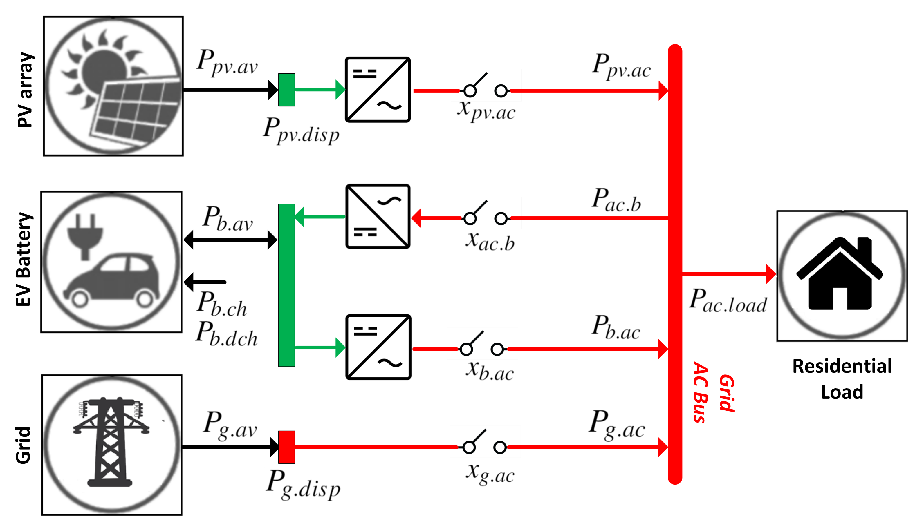
3.1. Home Area Power Network Architecture

The HAPN architecture under consideration is seen in Figure 2. The utility grid line is linked directly to the grid AC bus. Through inverters and a converter, the photovoltaic array and EV storage are connected to the grid AC bus. Controllable switches are included in the system to implement the nanogrid’s binary operations.
As shown in the figure, the grid supply power at the AC bus ( P g . a c ( t ) ) is:
P g . a c ( t ) m i n x g . a c ( t ) P g . d i s p ( t ) , P a c . l o a d ( t ) , t
where, x g . a c ( t ) { 0 , 1 } is the grid Boolean operator, P g . d i s p ( t ) is the controllable grid power, and P a c . l o a d ( t ) are the requested load demands. However, the electricity generated by solar panels P p v . a c ( t ) at the AC bus is limited to:
P p v . a c ( t ) m i n P p v . d i s p ( t ) , P a c . l o a d ( t ) + P a c . b ( t ) x p v . a c ( t ) η p v . c o n , t
where, P p v . d i s p ( t ) is the controllable PV power, P a c . b ( t ) is the power used to charge the EV battery, and η p v . c o n is the inverter efficiency.
Besides, the HAPN integrates a battery in the form of an electric vehicle acting as a storage entity having instantaneous available power ( P b . a v ( t ) ) that is limited to the maximum capacity of the EV battery ( E ¯ b ) such as:
P b . a v ( t ) E ¯ b / t . t .
the instantaneous power transfer from the attached EV to AC bus ( P b . a c ( t ) ) during discharging is:
P b . a c ( t ) = m i n η b . c o n P b . d c h ( t ) , η b . c o n P b . a v ( t ) , P a c . l o a d ( t ) x b . a c ( t ) , t
where, x b . a c ( t ) { 0 , 1 } , P b . d c h ( t ) is the battery discharge rate, and η b . c o n is the battery converter efficiency. However, the instantaneous power required for recharging the EV battery ( P a c . b ( t ) ) is illustrated in Equation (5), along with a Boolean operation of x a c . b ( t ) { 0 , 1 } .
P a c . b ( t ) = m i n [ P p v . a c ( t ) + P g . a c ( t ) P a c . l o a d ( t ) , η b . c o n 1 P b . c h ( t ) , E ¯ b / t ( η b . c o n 1 P b . a v ( t ) ) ] x a c . b ( t ) , t
where, P b . c h ( t ) is the charge rate of the battery. Besides, E b ( t ) is the battery capacity which is limited to its maximum E ¯ b and the minimum E ̲ b threshold:
E ̲ b E b ( t ) E ¯ b . t .
additionally, P b . c h ( t ) and P b . d c h ( t ) are restricted by a maximum and minimum value at any point in time, such as:
P ̲ b . c h P b . c h ( t ) P ¯ b . c h , t
P ̲ b . d c h P b . d c h ( t ) P ¯ b . d c h , t
besides, the AC bus exchanges power transfer as:
x p v . a c ( t ) P p v . a c ( t ) + x b . a c ( t ) P b . a c ( t ) + x g . a c ( t ) P g . a c ( t ) = x a c . b ( t ) P a c . b ( t ) + P a c . l o a d ( t ) + P d r v ( t ) . t .
in addition, one of the restrictions on battery operations is that the battery charging and draining activities cannot occur concurrently:
x b . a c ( t ) + x a c . b ( t ) 1 . t .
furthermore, the instantaneous state of energy ( E b ( t ) ) of the battery can be determined by:
E b ( t ) = E b ( t 1 ) + t 1 t ( ( η b . c o n ( P a c . b ( t ) + P d r v ( t ) ) · t ) ( η b . c o n 1 P b . a c ( t ) · t ) ) d t , t
where P d r v ( t ) is the power consumed by the EV during driving on road.

3.2. Battery Degradation Model

A common phenomenon of battery aging or degradation is observed during battery operations. There are two types of degradation that are commonly studied: (1) A reduction in a battery’s ability to deliver energy and (2) a reduction in the battery’s storage capacity. According to [39], the parameters involved in the above degradation phenomenon are high temperatures, high charge and discharge rates, and significant depth of discharge (DOD).
Jin et al. [40] created a reduced-order physical model to forecast the deterioration of lithium ion phosphate cathode and graphite anode battery cells. The storage cells under investigation have the individual capacity of 2.3 Ah, combining in series and parallel to construct a battery pack of a specific capacity power. The capacity loss due to the solid electrolyte interface (SEI) layer growth and active material (AM) loss are obtained at each time step t using Equations (12) and (13), respectively:
Q SEI ( t ) = t 1 t k SEI exp E SEI R T 2 ( 1 + λ θ ) t d t ,
Q AM ( t ) = t 1 t k AM exp E AM R T · SOC ( t ) · I b a t t , d i s c h ( t ) I b a t t , c h ( t ) d t .
A detailed description of the model is given in Appendix B.

3.3. Entities Cost Modeling

Real-time pricing (RTP) information is acquired from [41] in order to show the efficiency of dynamic grid pricing schemes ( θ ( t ) ) for demand side management (DSM) techniques in the HAPN. Whereas, the cost per watt for PV ( ϕ ( t ) ) and battery ( φ ( t ) ) operations is obtained from [42]. These operational costs are dependent on the installation and operation and management ( O & M ) costs. Additionally, O & M expense categories include inverter replacement, operations administration, module replacement, component replacement, system inspection and monitoring, module cleaning, land lease, property tax, and insurance, as well as asset management and security [42].

4. Problem Formulation & Numerical Solution

The HAPN is a single-phase power network that receives electricity from the utility grid, solar panels, and electric car batteries, and distributes it to house at a set voltage level. The paper illustrates energy allocation from different energy sources by implementing a cost-effective model predictive-based intelligent energy management strategy (MP-iEMS). This approach is used at the scheduling stage creating an output of set points for charging and discharging electric vehicles, feed-in from the PV, as well as grid power utilization. The energy management phase’s operational goal is to increase the customer’s satisfaction level and to improve the EV charging while keeping electricity operating costs as low as feasible. In addition, a hard constraint is introduced on meeting the users’ load needs. It ensures that the amount of energy supply is always equal or higher than the amount of energy demanded.
This means that priority should always be given to energy sources that provide relatively affordable power and that, if necessary, a portion of the EV charging load may be switched otherwise to balance the power. At each time t, the iEMS gains information about solar power, the state of electric car storage, and the load demands of users.
The objective is to develop a scheduling method u ( t ) { u x ( t ) , u p ( t ) } , that balances electricity from the grid, photovoltaics, and an electric vehicle battery. Whereas u x ( t ) = [ x p v . a c ( t ) , x b . a c ( t ) , x g . a c ( t ) , x a c . b ( t ) ] represents Boolean decision variables. The above variables indicated in Section 3 reflect the availability of diverse energy sources at the start of every iteration the algorithm runs and is illustrated as:
x g . a c ( t ) = 1 i f P g . a v ( t ) > P g . d i s p ( t ) 0 o t h e r w i s e , x b . a c ( t ) = 1 i f P b . a v ( t ) > E b ̲ ( t ) 0 o t h e r w i s e , x a c . b ( t ) = 1 i f P b . a v ( t ) < E b ¯ ( t ) 0 o t h e r w i s e , x p v . a c ( t ) = 1 i f P p v . a v ( t ) > P p v . d i s p ( t ) 0 o t h e r w i s e .
Thus, the aforementioned discrete variables contribute to the decrease in computing complexity by enabling an earlier decision on whether or not the particular supply source shall be activated. Furthermore, u p ( t ) = [ p p v . a c ( t ) , p b . a c ( t ) , p a c . b ( t ) , p g . a c ( t ) ] represents a vector of continuous power control variables for multiple energy sources. The aforementioned management policy is used to build a load and supply balance, taking into account the cost scenario for running HAPN. As a result, two distinct formulations of the problem are discovered:
P = min u ( t ) t = 1 T { θ ( t ) · x g . a c ( t ) P g . a c ( t ) + ϕ · x p v . a c ( t ) P p v . a c ( t ) + φ · x b . a c ( t ) P b . a c ( t ) } s . t . ref ,   Equations   ( 1 )   and   ( 2 ) ,   ( 4 ) ( 14 ) ,   ( 16 )   and   ( 17 ) .
The first is the cost minimization problem illustrates in Equation (15), and the second is the energy balancing problem shown in Equation (17), in which the house’s load requirements (according to Equation (16)) must be satisfied using the minimum amount of power. This problem can be resolved by implementing some of the security limitations discussed in the previous section. The power requirements ( P t a r g e t ( t ) ) for each time slot t, on the other hand, must be satisfied by a mix of power supplied by different sources. As a result, the following principles define the energy balancing constraint inherent in accomplishing the above mentioned goal. Hence, the target power that must be achieved for all timesteps t is illustrated as:
P t a r g e t ( t ) = max ( 0 , P a c . l o a d + x a c . b ( t ) P a c . b ) , i f x p v . a c ( t ) | x b . a c ( t ) | x g . a c ( t ) = 1 0 , o t h e r w i s e
The iEMS strategy prioritizes the use of PV energy. Consequently, if it is unable to meet the load requirements, the battery power is used. Otherwise, energy may also be fed in from the grid if necessary. The net power, allocated at any time slot t will be:
P p v . a c ( t ) + P b . a c ( t ) + P g . a c ( t ) P t a r g e t ( t ) . t .

4.1. Algorithms and Implementation

We have demonstrated three unique operating techniques for supply-side management that may be compared to achieve the best results. Among them are the following:
1.
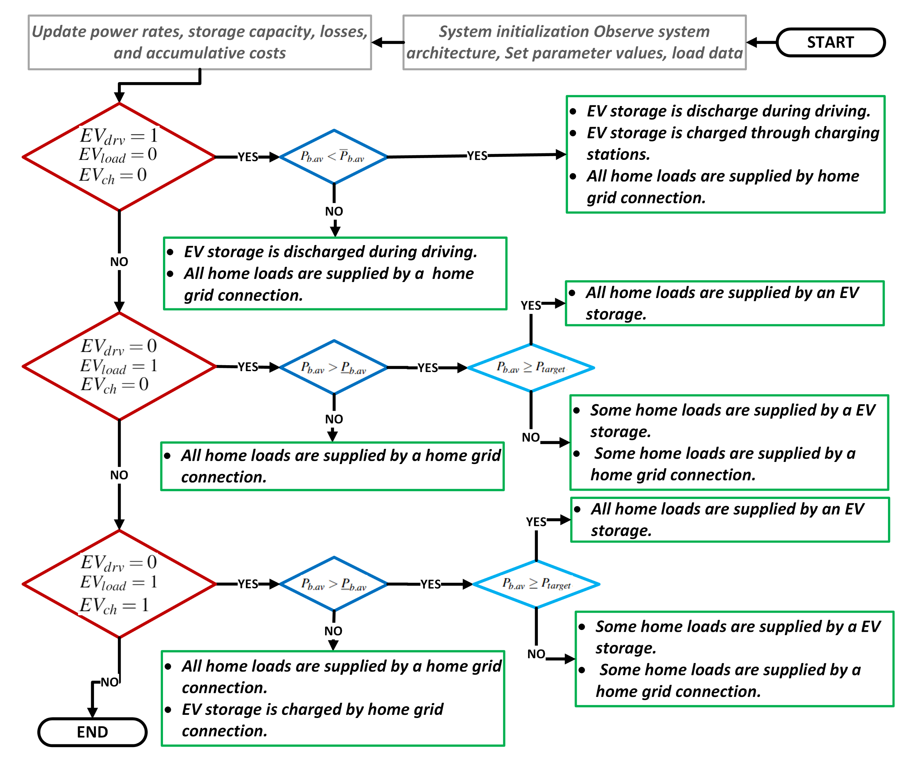
Scheme 1: Conventional rule-based strategy involves only the EV storage and grid energy supply (Conv-EG).
2.
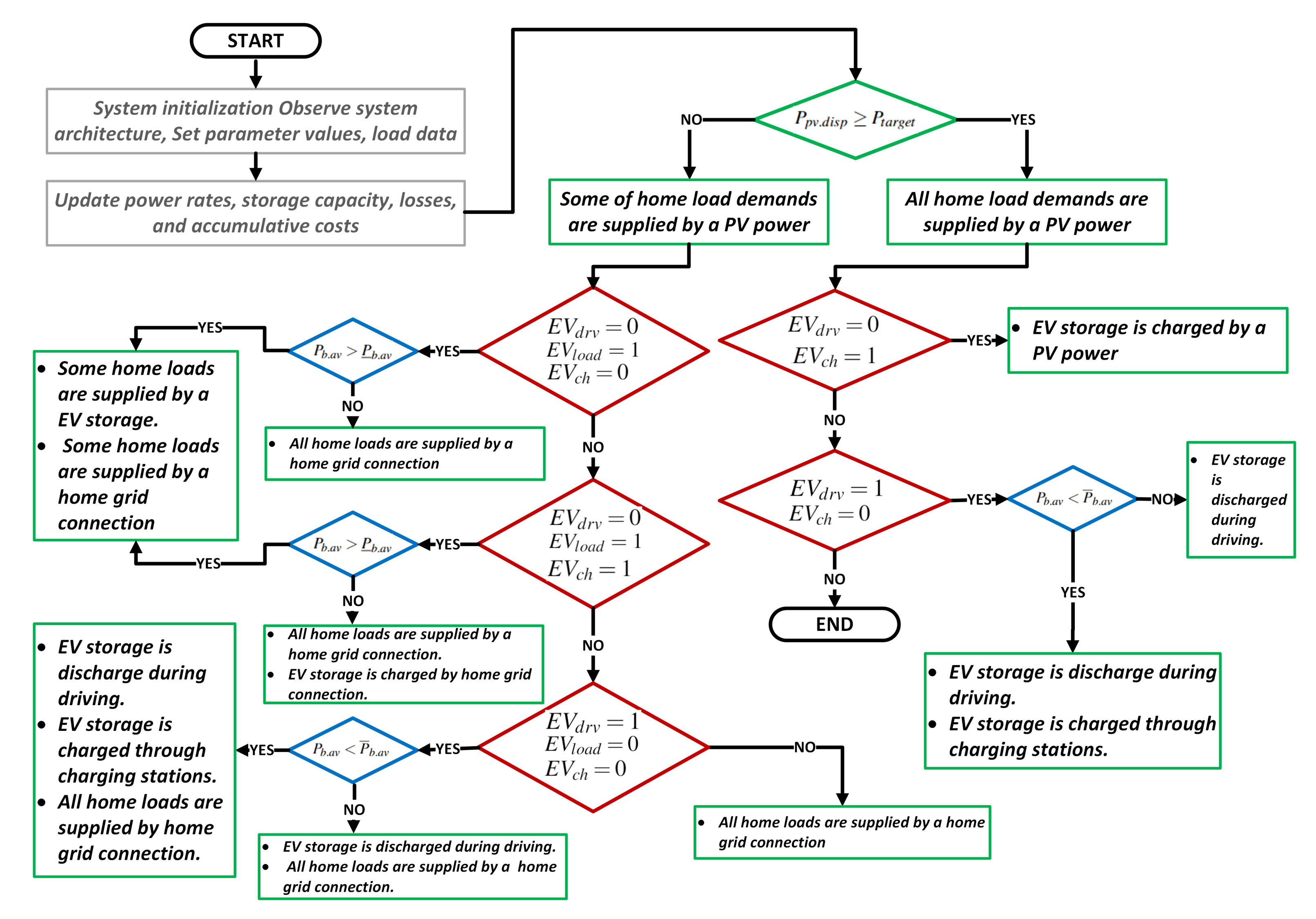
Scheme 2: Conventional model predictive rule-based strategy involves PV supply along with EV storage and grid energy supply (Conv-PEG).
3.
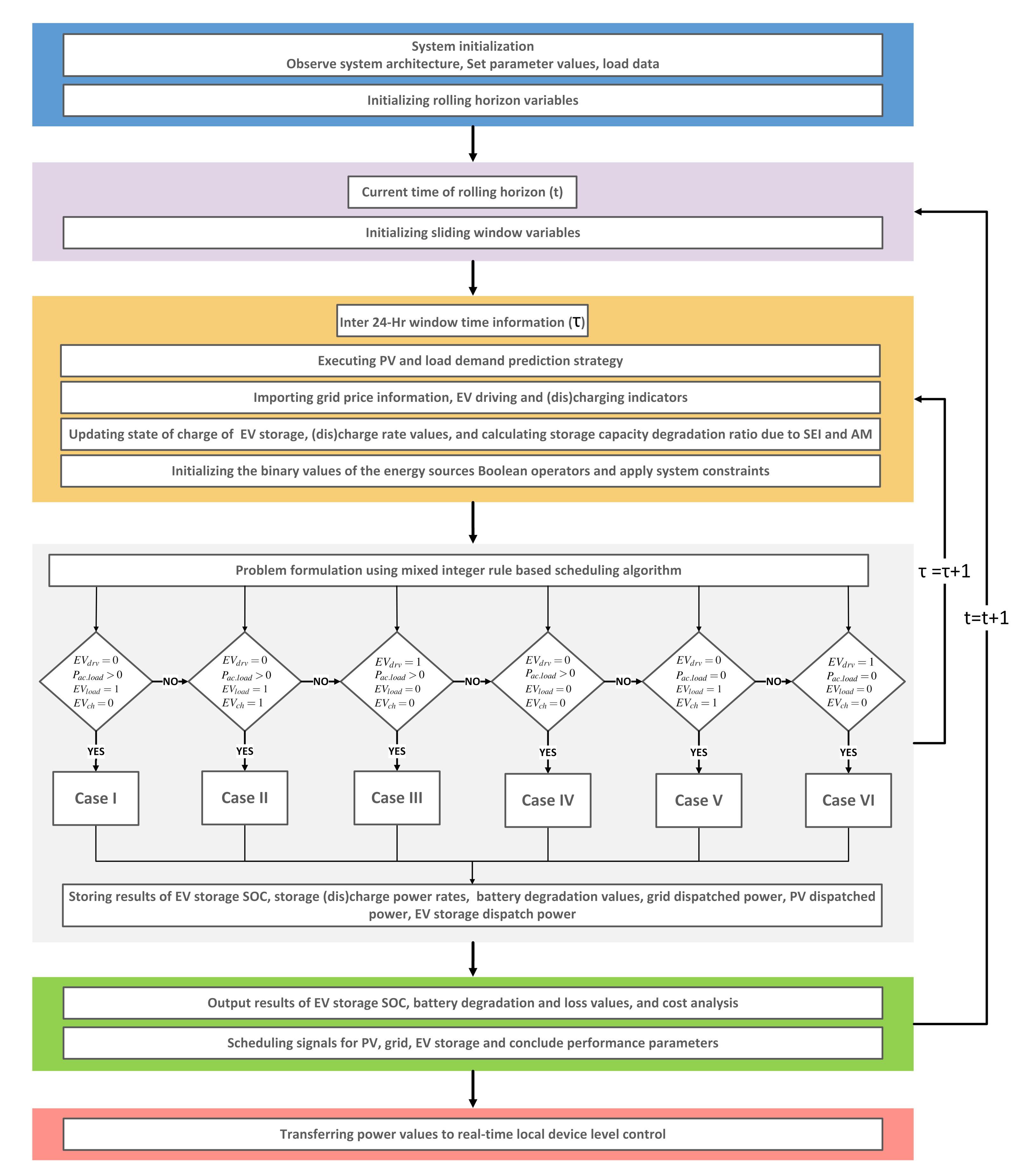
Scheme 3: Proposed Model predictive intelligent energy management system (MP-iEMS).
For all three optimization schemes, the system model is identical to that presented in Section 3, except that the PV is missing in Scheme 1.
To address the concerns expressed in (15) and (17), we suggest a set of establishing priorities for acquiring power values from the absolute cheapest and most dependable source of energy. This set includes two continuous power indicators and three binary indicators. One of the power indicators cover both the actual load and storage charging requirements ( P t a r g e t ( t ) ) and the other is EV consumption when driving ( P d r v ( t ) ). While binary indicators such as drive bool ( E V d r v ( t ) { 0 , 1 } ), electric vehicle charging Bool ( E V c h ( t ) { 0 , 1 } ), and electric vehicle loading Bool ( E V l o a d ( t ) { 0 , 1 } ) are also accessible. The feasible solution set is composed of 16 distinct conditions based on these four indicators. Only six of them seem plausible, and we used a rule-based expert system to apply them over the operating window. The remaining 10 candidate sets are not feasible operationally and so cannot be adopted. Consider the following binary loading signals when developing the control policy u ( t ) , as they are already contained in data sets.

4.1.1. Scheme 1: Conv-EG

The scheduling strategy (Conv-EG) is a priority-based decision algorithm as shown in Figure 3. We assume that the system model used to apply this algorithm only contains a supply from the grid and EV storage. In this algorithm, the EV storage has priority over the grid to supply power to the load demands. It is due to the assumption that the EV storage might be charged at low peak hours at comparatively lower rates. Hence, at the initial stage, EV storage is analyzed to determine whether it can fulfill the load demands completely by itself or not. If the EV is parked at home and the loading Boolean is enabled, it will automatically discharge. Additionally, if the charging Boolean is active, then it is capable of charging as well. However, if the EV drive Boolean is set to true, the EV will drive on the road and will charge itself via charging stations, while the home loads will be provided by grid electricity. The detailed workflow of the algorithms is illustrated in Figure 3.

4.1.2. Scheme 2: Conv-PEG

The scheduling method (Conv-PEG) incorporates a rooftop photovoltaic system. As a result, the working framework contains an additional low-cost source of power as seen in Figure 4. In this algorithm, the PV source is considered to be the cheapest source of energy, as it requires only solar energy to generate freely available power. The Conv-PEG is initiated by initializing the decision window’s system variables and anticipating new values for PV in-feed and load demands. Additionally, it updates the battery’s state of charge (SOC), charging power rate, and battery capacity.
Thus, the algorithm’s first step determines if there is enough photovoltaic power available to meet the needs of the customers. If the answer is “yes”, the PV meets all of the load needs for the time period t right away. Then it comes to the binary indicators, and analyses if the electric cars can be charged at home or on the road. If it is at home, the PV power that is not used to meet the needs of the load can be used to charge the battery. The battery would then be charged until it reaches its full capacity or until it gets as much power from the PV as it can. It is important to note that the grid is disconnected during this process. However, if the car is on the road, there are two possibilities. It may be able to charge itself while on the road if it comes across a charging station. Otherwise, it will continue until it runs out of charge.
In comparison to the previous choice, if the available PV capacity is less than the load demand, and the needs are partially met by the PV power, using EV storage becomes a secondary consideration if it is available for discharging as shown in Figure 4. While, in the worst-case scenario, the remaining unsatisfied loads are fulfilled by the grid. The grid will deliver power on a demand basis and charges according to the market price of energy. Similarly, while the EV is at home and linked to the HAPN, the EV acts as temporary storage. The home will benefit from this EV storage by balancing and providing low-cost electricity during periods of poor solar production and high grid costs. Additionally, during periods of high solar energy output, this EV may charge itself using the HAPN battery charging system.

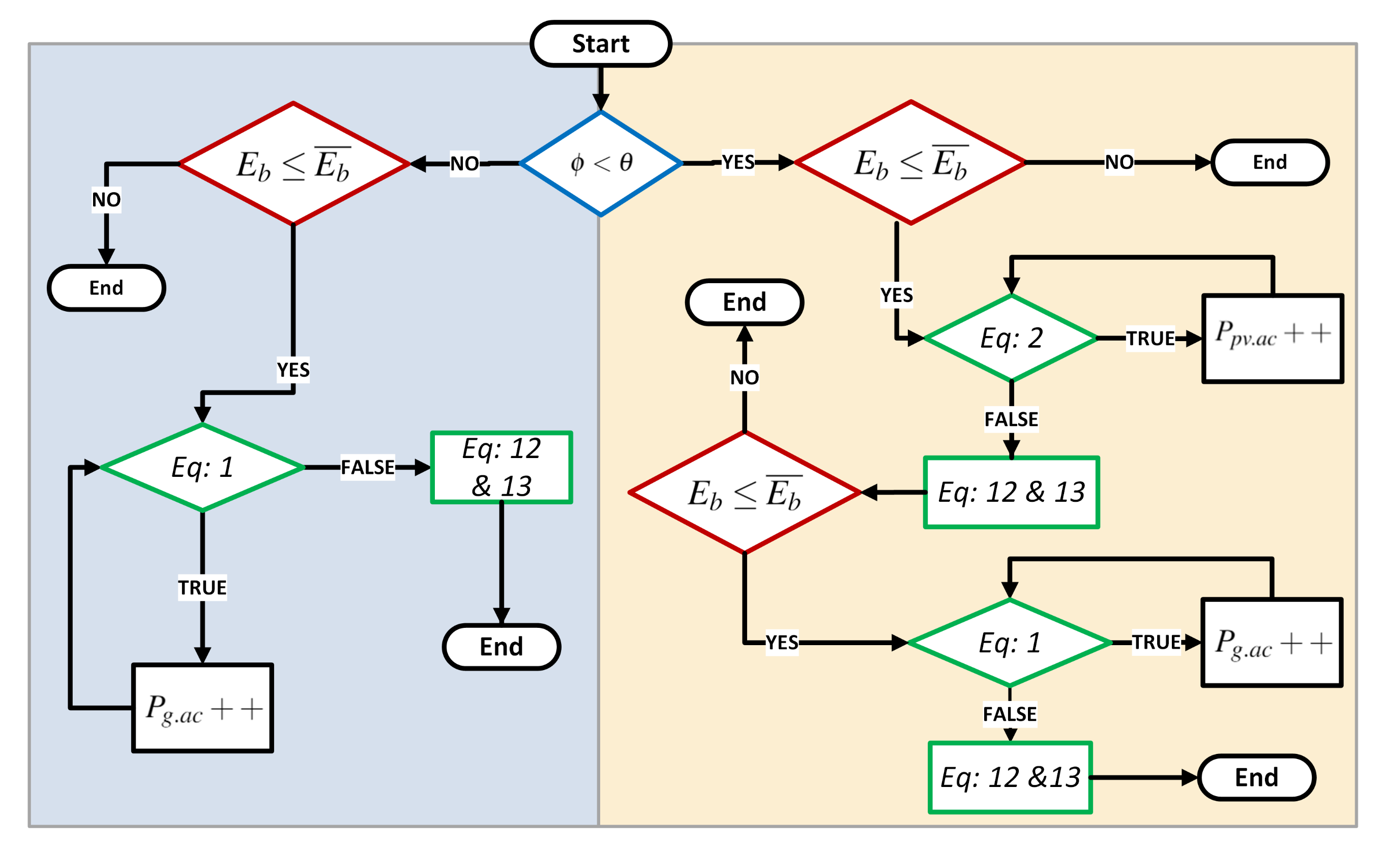
4.1.3. Scheme 3: MP-iEMS

The authors propose a two-stage model predictive iEMS framework with a hierarchical structure. The first stage involves developing an energy scheduler to guarantee that the net cost of energy generated is kept to a minimum. It combines a predictive sliding window module with a rule-based decision algorithm that runs at a sample rate of 15 min, i.e., t [ 1 , 2 , , T ] . While the sliding window has a time resolution of 24 h i.e., τ ( t + 24 ) . Additionally, the second stage utilizes a current-controlled current source to activate the ESEs based on the decision signals acquired. This stage runs at a much higher sample rate of 1 s, i.e., k [ 1 , 2 , , K ] , reflecting the electrical devices’ real-time activity. The suggested MP-iEMS is schematically represented in Figure 5, which depicts the rolling horizon rule-based decision approach.
As shown in Figure 5, initially, the system architecture is observed, system parameters are configured, input data are loaded, and rolling horizon control variables are defined. The current time of the rolling horizon t is then established, and the sliding window’s settings are set. Additionally, a 24-h sliding window with a k time resolution is explored for the application of a rule-based decision method. At each instantaneous time step, the MP-iEMS is initiated by initializing the decision window’s system variables and anticipating new values for PV in-feed and load demands. Additionally, it updates the battery’s state of charge SOC, charging power rate, and the capacity of the battery. The operating window is executed using a receding horizon technique, with the next step t sliding over every 15 min. Through implementing this strategy, the decision values of the control variables for the whole year may be derived.
To solve the problem described in Equation (15), the priority criteria for getting power values from the least expensive and most dependable energy source choice is introduced. The algorithm suggests alternative cases that are defined in accordance with the scenarios produced using the data set’s system input parameters. To create the control policy u ( t ) , the following scenario configurations can be considered:
1.
Case 1: E V d r v ( t ) = 0 & P a c . l o a d ( t ) > 0 & E V l o a d ( t ) = 1 & E V c h ( t ) = 0 :
2.
Case 2: E V d r v ( t ) = 0 & P a c . l o a d ( t ) > 0 & E V l o a d ( t ) = 1 & E V c h ( t ) = 1 :
3.
Case 3: E V d r v ( t ) = 1 & P a c . l o a d ( t ) > 0 & E V l o a d ( t ) = 0 & E V c h ( t ) = 0 :
4.
Case 4: E V d r v ( t ) = 0 & P a c . l o a d ( t ) > 0 & E V l o a d ( t ) = 0 & E V c h ( t ) = 0 :
5.
Case 5: E V d r v ( t ) = 0 & P a c . l o a d ( t ) = 0 & E V l o a d ( t ) = 1 & E V c h ( t ) = 1 :
6.
Case 6: E V d r v ( t ) = 1 & P a c . l o a d ( t ) = 0 & E V l o a d ( t ) = 0 & E V c h ( t ) = 0 :

Case I

This case is reflected in Figure 6, which indicates that the EV is parked at home and is attached to HAPN to supply power to the home appliances. However, the charging bool of EV is inactive and it cannot be charged by any means, however it can be discharged to satisfy the load demands. Furthermore, the load demands can also be supplied by the PV and grid power. To supply power from the cheapest source of energy, per unit energy prices are first compared between the PV, EV battery, and grid power sources (i.e., ensuring Equation (15)). If the PV power price is the cheapest, then power is drawn from the PV source until the demand is met or there is no further power available from PV. If the demand still persists, then the next power source is selected based on the cheap unit price. If the power from the battery is cheap and the SOC of the battery is above the threshold, then the power is obtained from the battery. Otherwise, the loads are met by the grid power as a worst case scenario. It is worth noting here that grid prices are dynamic, and the cost per unit can be lower than the cost of energy acquired from the PV or battery in some cases.

Case II

The flow chart for the case II strategy shown in Figure 7 indicates that the working principle of this case is quite similar to that of case I when supplying power to the load demands. The only difference is the activation of charging the EV battery at the HAPN. Hence, the battery could be charged using PV power or grid power. The flow chart indicates that if the user’s load demand is completely fulfilled by the PV power, then the remaining PV power could be used to charge the EV until the battery is fully charged or up to the limit of PV production. However, if the PV power does not fulfill the battery charging requirements, then the grid comes into action and charges the battery until it is charged to its limit.

Case III

Here, it shows the drive Boolean of the EV, meaning the vehicle may drive out of the home. Thus, it is also evident that now the EV storage would only be used for driving purposes. However, in the meantime, there is also a need to fulfill the load demands of the household. Therefore, the options available to satisfy the demands are the utilization of the PV and grid power. Again, based on the cost comparison, a scheduling decision is made on whether the power should be obtained from PV or the grid (i.e., ensuring Equation (15)). In this case, because the EV is not attached to the HAPN, there is no opportunity for charging and discharging the EV storage. The flow chart for case III is illustrated in Figure 8.

Case IV

As shown, Figure 9 indicates that the vehicle is at home but is not participating in the demand response program. This means that the EV storage will not charge or discharge itself to fulfill the load demand requirements at the HAPN. Hence, in this case, the EV user gives up the decision of utilizing EV storage to satisfy the additional constraints i.e., to save battery life. In this case, the user’s power demand is satisfied by PV and the grid power, opting the lowest possible cost scenario (i.e., ensuring Equation (15)).

Case V

In this case, the electric vehicle that is parked at the home, is attached to the home power grid, and participates in a demand response program for a HAPN. However, here it shows in Figure 10 that there are no user’s power requests to be fulfilled at the moment, but the EV has the option to take advantage of the situation and charge itself using a low cost power provider (i.e., ensuring Equation (15)). Hence, if the cost of power dispatched from PV is lower and the storage has the capacity to charge itself, then the EV battery will be charged by the PV source until it is fully charged or the PV source is depleted. In the worst case, the battery may be fully charged by grid power at any cost.

Case VI

Case VI in Figure 11 illustrates that the EV is on the road and uses its storage only for driving purposes. Moreover, there are also no power requests back at home. Hence, the PV power is curtailed if any and no grid power is requested at this time.

4.2. Evaluation Indices

To evaluate the system’s performance and to determine the best combination of various energy resources, the following important performance metrics are defined:

PV Utilization Factor ( K P V . U F )

This refers to the ratio of the total PV power utilization to satisfy the load demands to the total available PV power. In the previous section, it is demonstrated that the actual PV power utilization is always less than that of the available and it is due to the losses induced in the converter. It can be illustrated as:
K P V . U F = P p v . a c ( t ) P p v . a v ( t ) .

PV Penetration Level ( K P V . P L )

This describes the ratio of the total PV power used to satisfy the portion of load demands that make up the total power demands of a home. This can be elaborated as:
K P V . P L = P p v . a c ( t ) P a c . l o a d ( t ) + P a c . b ( t ) .

Grid Utilization Factor ( K G . U F )

This refers to the ratio of the total grid power utilization to satisfy the load demands to the total available grid power. In the previous section, it is demonstrated that the actual grid power utilization may be less than that available and is due to the request of HAPN. It can be illustrated as:
K G . U F = P g . a c ( t ) P g . a v ( t ) .

Grid Penetration Level ( K G . P L )

This describes the ratio of the total grid power used to satisfy the portion of load demands that is lesser than the total power demands of a home because of the involvement of the PV and EV battery. This is elaborated as:
K G . P L = P g . a c ( t ) ( P a c . l o a d ( t ) + P a c . b ( t ) .

EV Storage Utilization Factor ( K E V . U F )

This refers to the ratio of the total power discharged from EV storage to fulfill the house energy requirements to the total capacity of the storage and the extra power being charged in the EV battery. In the previous section, it is demonstrated that the actual storage power utilization in HAPN is always less than that available. It is due to the losses induced due to conversion losses. Moreover, most of the energy is used for driving purposes. It can be illustrated as:
K E V . U F = η b . c o n 1 P b . a c ( t ) ( P b . a v ( t ) + η b . c o n P a c . b ( t ) ) .

EV Storage Penetration Level ( K E V . P L )

This describes the ratio of the total discharge power from the EV storage used to satisfy the portion of load demands. This can be elaborated as:
K E V . P L = η b . c o n 1 P b . a c ( t ) P a c . l o a d ( t ) .

Degree of Self-Sufficiency ( K S S )

The degree of self-sufficiency refers to the ratio of the total energy consumption that is covered by the PV and EV storage and is defined as:
K S S = ( P l o a d ( t ) P g . a c ( t ) ) P a c . l o a d ( t ) .

5. Case Study & Simulation Results

The suggested iEMS techniques are being assessed on several performance metrics stated in Section 4.2 to demonstrate its actual capability. Along with this, a comparison of HAPN operational costs to conventional rule-based optimal approaches is made. In addition, a real-world annual data set [43] of EV storage (dis)charging, PV power, and grid energy pricing is utilized to supply input data to the algorithms. These approaches then determine the actual optimal output power levels for each energy supply entity. The parametric values for the various power entities contained in our system model are summarized in Table 2.
The cost associated with various ESEs is examined during scheduling process to obtain the ideal outcome. The dynamical grid energy cost, which fluctuates with time t and is depicted in Figure 12, is the most crucial cost parameter. Furthermore, as stated in Section 3.3, there are certain fixed operating and maintenance expenses connected with PV operations and EV storage consumption. Furthermore, the parameters linked with the deterioration of the specifications of the EV battery bank are provided in Table 3.
The suggested MP-iEMS is intended to demonstrate the scheduling framework’s response for the whole year on the receding time horizon of 15 min. The algorithm that seeks the lowest cost also seeks to improve a HAPN’s self-consumption and self-sufficiency. Forecasting of PV power generation and user load demands are the important components of the entire process. Additionally, minimum and maximum energy limits are established for matching energy supply and demand entities in order to define a realistic operating range.

5.1. Data Preparation

The complete dataset for one year used in the simulations has been published by Rheinberger [43]. It comprises of the following subsets:
  • Day-ahead energy market prices for the bidding zone Germany-Austria-Luxembourg [44];
  • Photovoltaic production in a localized place in Germany [41];
  • Photovoltaic production prediction [45];
  • Electric vehicle usage from the UK [46];
  • Household demand from Ireland [47].
MATLAB/Simulink is used to simulate the data and the given data sets have to be converted according to the workaround described in Appendix A. Whereas, Figure 12 shows the actual auctioned day-ahead energy price information.

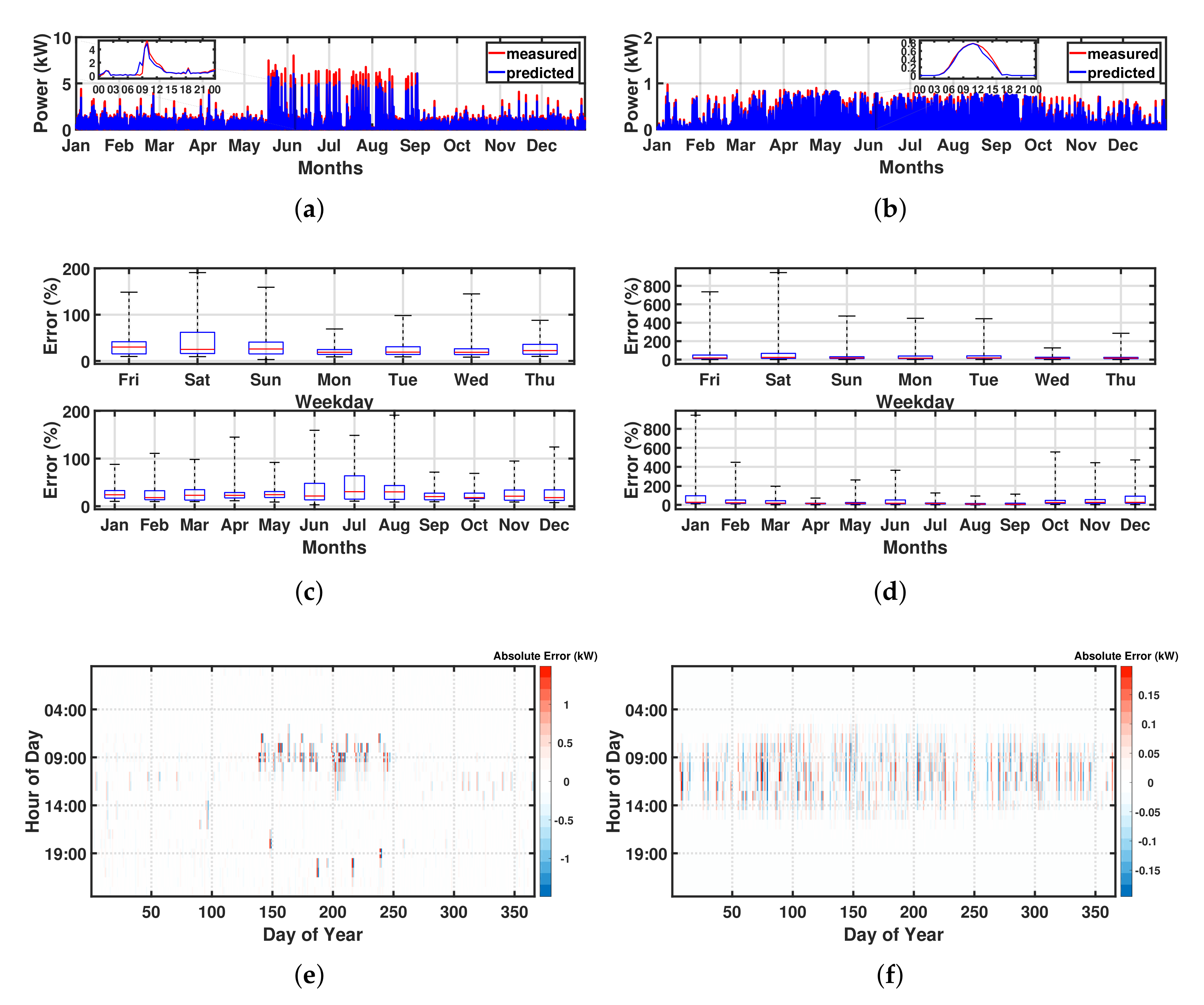
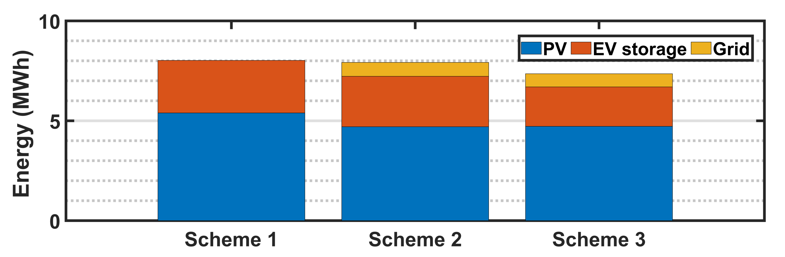
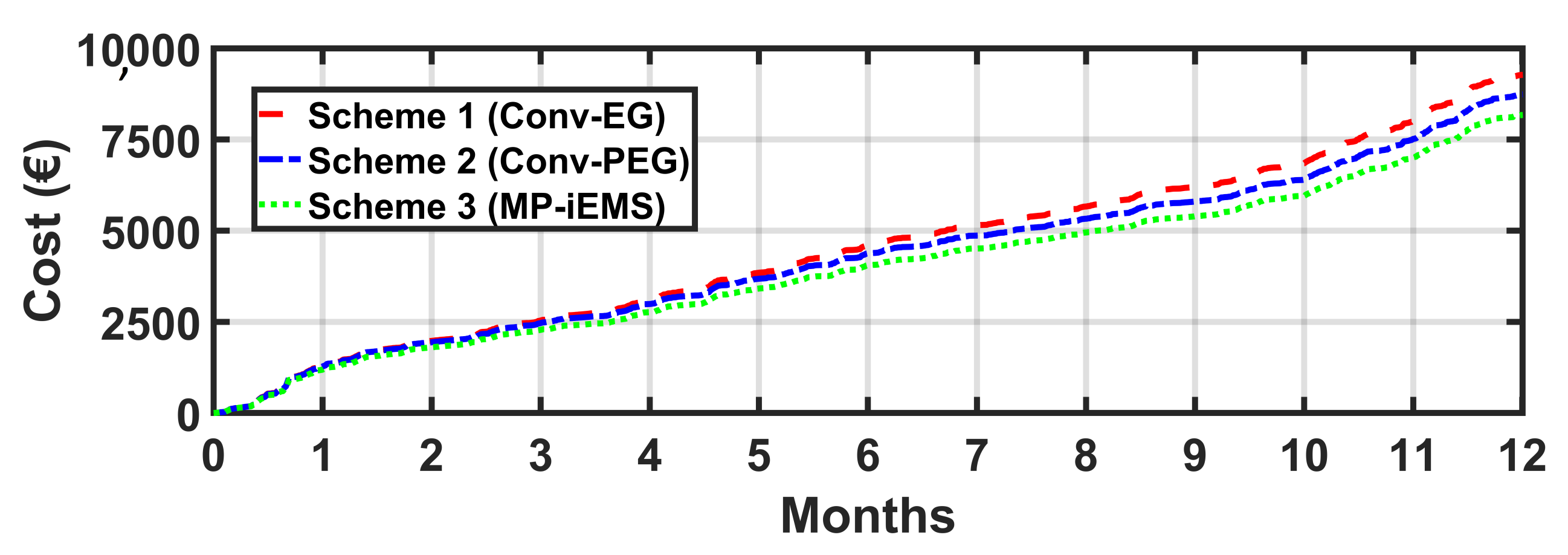
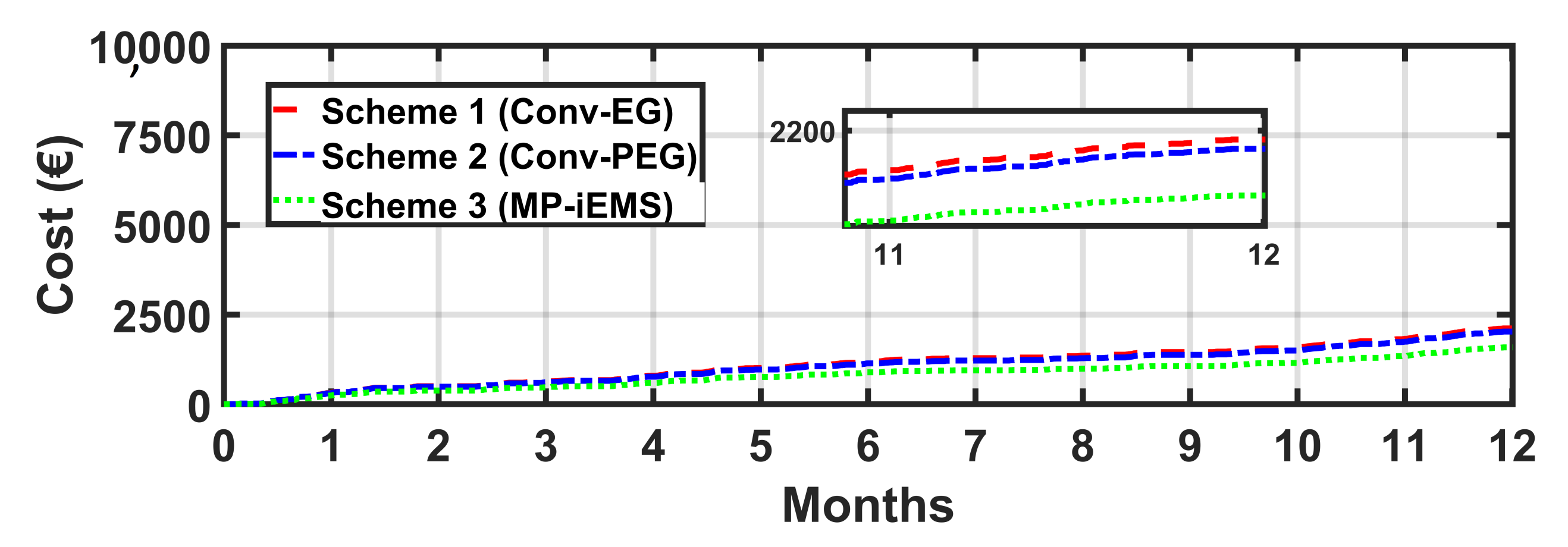
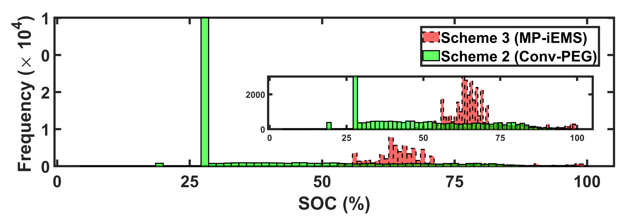
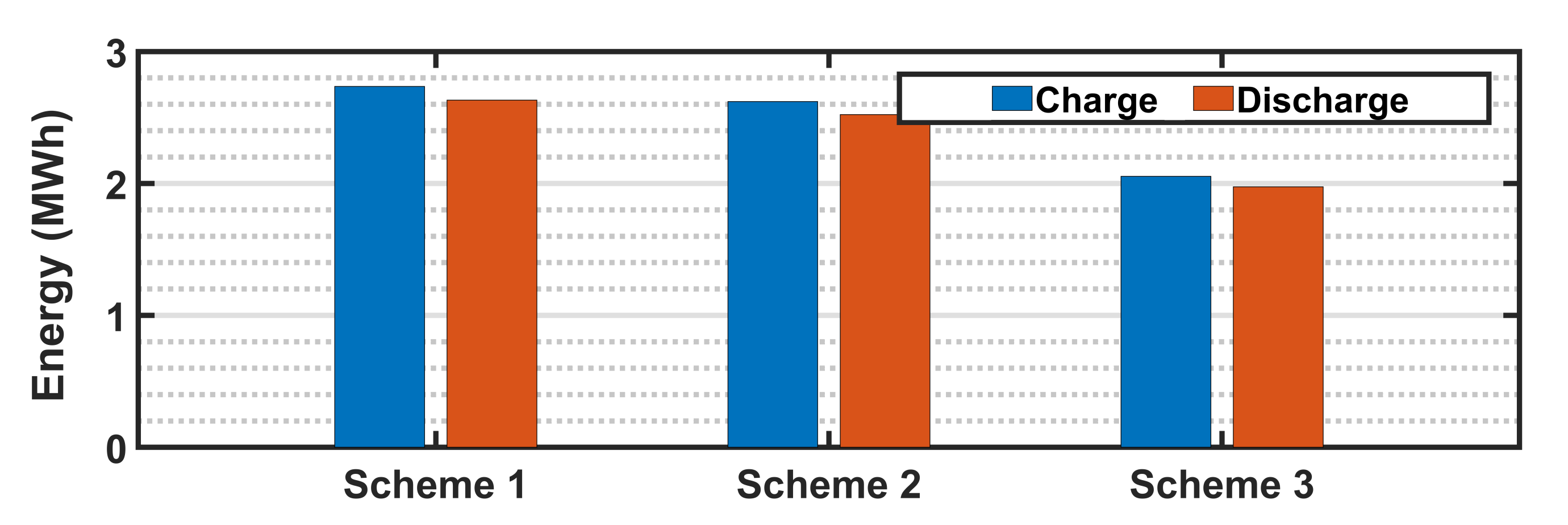
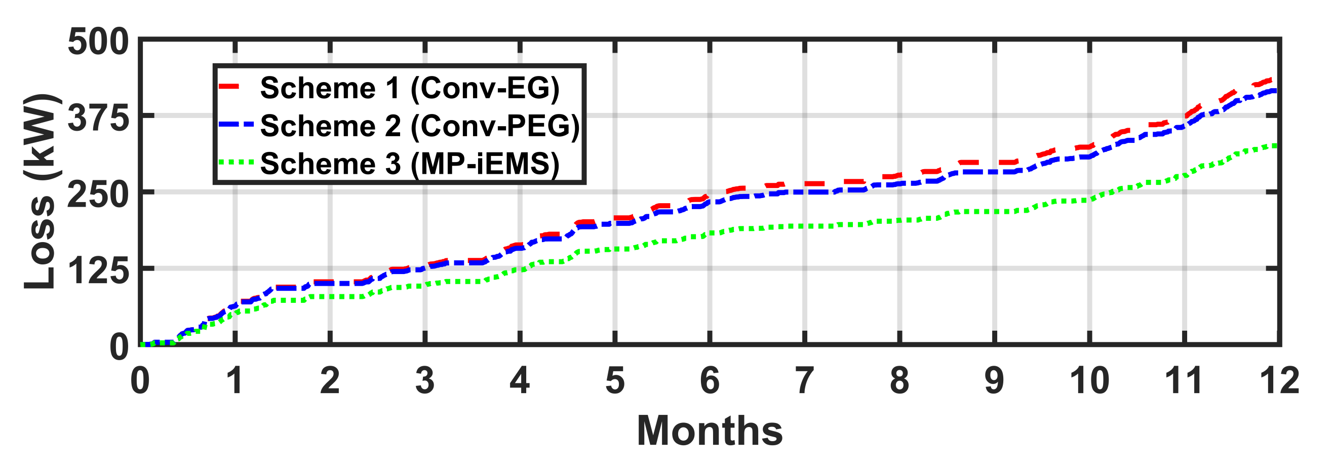
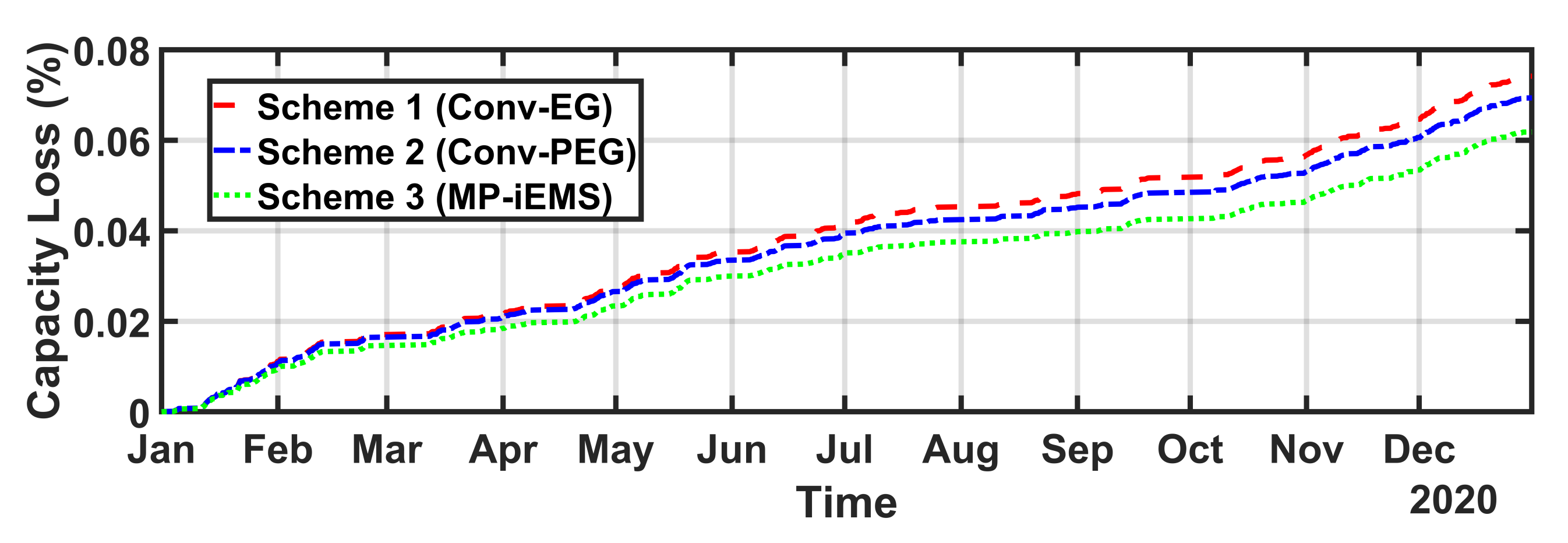
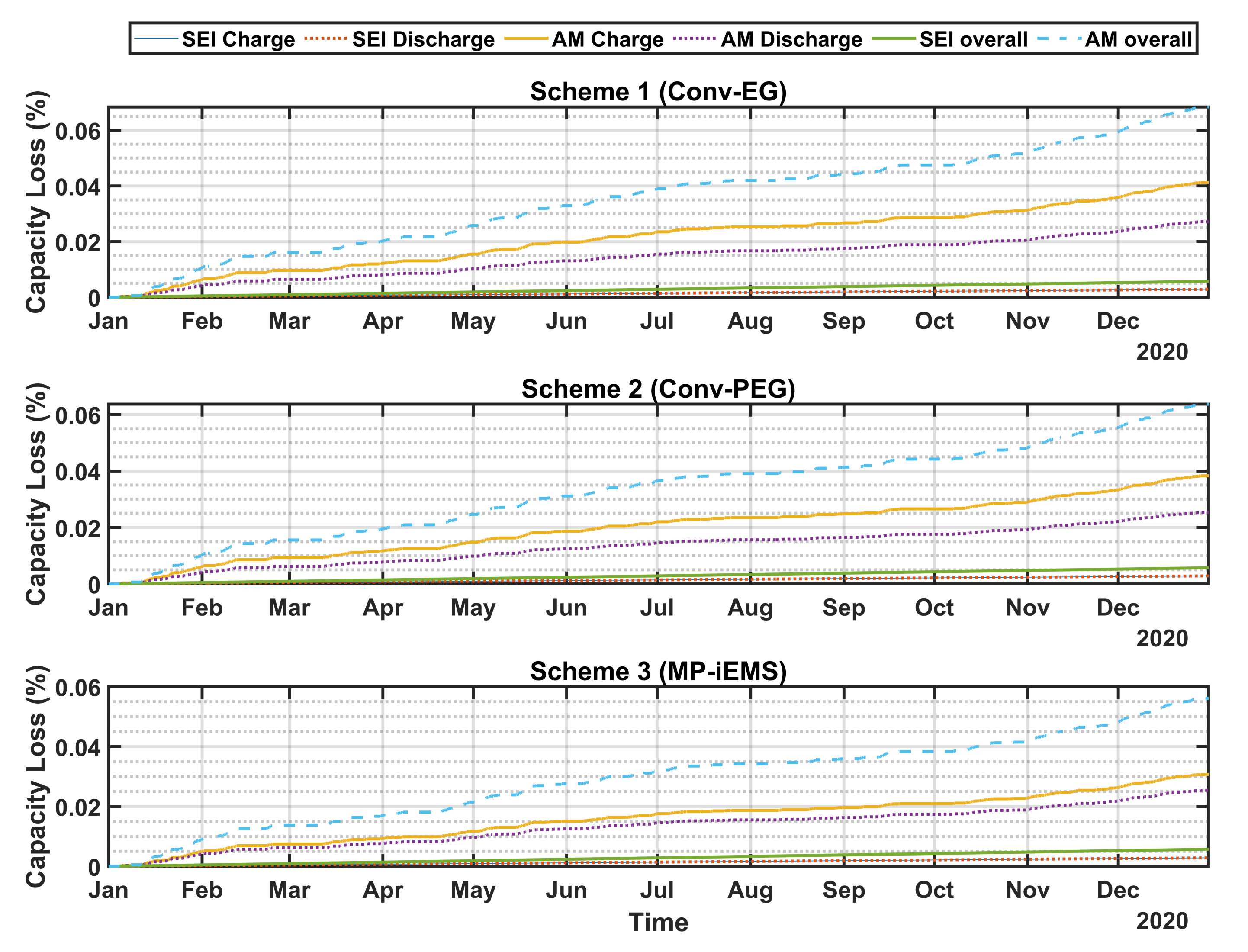
5.2. Comparative Analysis of Power Scheduling Schemes

Within the scope of supply side management, we have examined and compared the operating expenses of various energy supply entities. We chose three distinct operating strategies to compare for the best outcomes. Among these are: (1) Scheme 1: Conv-EG, (2) Scheme 2: Conv-PEG, and (3) Scheme 3: MP-iEMS.
Schemes 1 and 2 represent greedy priority-based algorithms. In which attention is given to a low-cost energy source such as PV and EV storage. Scheme 3, on the other hand, makes use of intelligence by anticipating future changing grid energy costs and optimizing the capacity usage of EV storage and the PV source. All of these techniques provide for the required power to be accessible from any supply entity at the lowest feasible cost, while also ensuring maximum comfort for energy users by meeting their demands with their immediate energy requests, as indicated in Equation (17).
Initially, an examination of several performance measures is presented that are previously mentioned in Section 4.2. Table 4 compares the indices for various ESEs among various optimum schemes.
It shows that the typical optimum scheme that does not incorporate PV has a high grid utilization factor ( K G , U F ) and penetration level ( K G , P L ) when compared to other schemes, which is understandable. Nevertheless, the grid usage factor for Schemes 2 and 3 is nearly the same. However, the grid penetration level in Scheme 2 is high, indicating that Scheme 3 uses grid electricity a slightly less than Scheme 2. Furthermore, the PV usage factor ( K P V , U F ) in Scheme 2 is high, even though the penetration level ( K P V , P L ) in both schemes is very similar. It demonstrates that in Scheme 3, when grid prices are negative, as shown in Figure 12, the MP-iEMS algorithm disconnects the PV and instead obtains energy from the grid. This would also reduce energy conversion losses from DC to AC, thereby increasing the shelf life of PV modules. Furthermore, the EV usage factor ( K E V , U F ) is about identical for Schemes 1 and 2, while it is somewhat lower in Scheme 3. Similarly, the penetration level of the EV storage ( K E V , P L ) is also lower in Scheme 3, which indicates that the MP-iEMS algorithm engages the EV operations sporadically in comparison to Scheme 2. In this way, the storage has been utilized more efficiently. In comparison, the self-sufficiency indicator ( K S S ) is high in Scheme 2, where the operations of PV and EV storage are involved more often. However, due to the optimal and efficient utilization of PV and EV storage, this factor is less in Scheme 3 while it is at its lowest in Scheme 1 due to the absence of the PV energy source.
In addition, Figure 13 depicts the comparative contribution of various ESEs in various energy optimal schemes. Where Scheme 3 uses less energy overall due to lower energy losses incurred during battery and PV operations.
We also investigate the yearly accumulative price of the energy associated with grid power utilization, PV usage, and EV storage utilization as shown in following figures. Figure 14 demonstrates that Scheme 3 has overall exhibited a lower energy cost, followed by Schemes 1 and 2, respectively. Scheme 1 exhibits high costs due to the absence of a cheap energy source, i.e., PV, as shown in Figure 13. The load demands are satisfied exclusively by grid power, where the grid power is also used for charging the EV storage when needed.
Figure 15 and Figure 16 refer to the high grid cost and storage operating cost for Scheme 1, respectively. It may be due to the high charge and discharge rates associated with high grid energy prices.
On the other hand, in Scheme 2, the PV source is added. It is then utilized to satisfy the loads along with charging the EV storage when the grid energy prices are high and extra power is available from the PV source. However, both of these schemes opt for the same price for the EV operational costs, and so the storage utilization is almost the same.
Furthermore, in Scheme 3 the system model is similar to that of Scheme 2 where the cheap PV source is included, however in this scheme, an extra intelligence is placed to look into the cheapest option of energy available at any instance of time. As seen in Figure 12, sometimes the grid energy prices become negative or gaining energy from the grid is sometimes cheaper as compared to the energy obtained from the PV (i.e., due to operational and maintenance costs). Hence, our proposed MP-iEMS algorithm used in Scheme 3 can have this intelligence about when to use PV or when it is cheap to utilize grid power both for satisfying user load demands and charging the EV. One can see in Figure 13 that the PV utilization is lower in Scheme 3 in comparison to Scheme 2. It takes more energy from the grid at the lowest possible price and still exhibits a quite lower grid energy price when looking into the zoom window of Figure 15. However, on the other hand, this scheme also utilizes EV storage quite efficiently and achieves the lowest battery operational costs as compared to other schemes as shown in Figure 16.
Moreover, if we want to know the difference in the behavior of utilizing EV storage especially for Scheme 2 and Scheme 3, a histogram of state of charge (SOC) in Figure 17 shows that Scheme 2 maintains a quit low range of SOC in between 25 % to 75 % . While Scheme 3 maintains this SOC approximately in between 55 % to 75 % . It indicates that Scheme 2 experiences deep discharges and high battery utilization as compared to Scheme 3.
Similarly, if we look into Figure 18, Schemes 1 and 2 opt for normally high charge rates around 23 kW, while Scheme 3 experiences low charge rates in comparison to other schemes around 12 kW.
Another comparison in terms of yearly accumulative charge and discharge energy for various schemes is shown in Figure 19. It demonstrates that Scheme 1 encounters a significant amount of energy exchange throughout the battery’s charge and discharge cycles. It is due to the absence of a third source of energy when compared to Scheme 2, where these values are comparatively low around 2.6 MWh, and it is due to the induction of the PV source. Which takes over some of the supply from EV storage. However, Scheme 3 experiences the lowest charge and discharge energy exchange of around 2 MWh, and it is due to the intelligence of utilizing the optimum share of energy from each source at a very optimal price.
Moreover, Figure 20 demonstrates the accumulative EV storage losses. These losses are evident during the charge and discharge of EV storage and are due to the inefficiency of the conversion (i.e., AC-DC or DC-AC). As illustrated above, Scheme 3 experiences less EV storage utilization, so it also exhibits less storage loss as compared to Scheme 2 and 3. It is worth mentioning that the driving behavior and EV consumption on the road are the same for all the study schemes. However, there are differences in the number of times the EV battery is charged and discharged
Furthermore, EV storage capacity loss analysis is carried out to demonstrate the effects of dynamic storage SOC and (dis)charge rates. This loss analysis is done using the battery model data available from [40]. The battery SOC, charge/discharge power, and the elapsed lifespan are all inputs into the storage degradation model, which then determines the percentage capacity loss. Degradation models are usually complex and non-linear.
Figure 21 shows the variations in the accumulative capacity loss of the storage for the whole year. While Figure 22 illustrates individual scheme-based capacity losses induced due to charge, discharge, and the SOC of the storage. Moreover, two types of losses (e.g., SEI and AM capacity loss) are shown individually for every scheme.
All three systems have AM losses greater than SEI losses, as seen in the figure. The charging and discharging rates affect the AM losses, hence higher rates result in higher losses. With increasing SOC, such as Scheme, the AM capacity loss grows in a monotone pattern. The AM variation pattern is time-invariant since it is unaffected by the amount of time the battery has been in use. Due to high charge rates, AM charge losses are larger than AM discharge losses, especially when the car charges itself using the charging station’s high charge power option. SEI losses are reliant on the storage’s SOC, whereas SOC losses are independent. With increasing net discharge power, the SEI capacity loss reduces in a linear fashion. The battery run duration has an adverse effect on the SEI capacity decrease rate.
Compared to the other three schemes, the overall AM losses in Scheme 3 are lower. Scheme 2 and 3 have very little difference, on the other hand. However, there is not a significant difference in overall SEI losses between these schemes. This may be because there are not as many changes in SOC between them, and that the battery runs for a long time i.e., the whole year. In addition, a heat map can provide another perspective to analyze the losses during the hour of the day and the month of the year. Figure 23, Figure 24 and Figure 25 show the heat maps for Schemes 1–3, respectively. In all these schemes it is evident that the storage capacity losses are high in winter, especially during 3:00 p.m. to 8:00 p.m. It is due to higher driving utilization of battery during the winter season.

6. Conclusions

This article analyzes energy distribution by various energy resources in a HAPN on a multi-time scale. To make time-ahead cost effective scheduling decisions, the iEMS uses a receding horizon rule-based mixed-integer dynamic algorithm. It reduces spontaneous consumer’s energy costs by utilizing the cheapest available energy source at any instantaneous time while maintaining high customer comfort and improving HAPN self-sufficiency. The storage life-cycle deterioration phenomenon is also observed to increase the overall practical usefulness of the battery. However, for real-time device actions, the previously acquired decision values from the scheduler are fed into the device-level control. The proposed model predictive iEMS capabilities are demonstrated using real-life annual data sets for homes, EV driving patterns, and EV battery (dis)charging patterns. The proposed MP-iEMS Scheme has demonstrated that by incorporating dynamic energy prices, the total energy demands are fully met by the energy obtained from the cheapest power source. Additionally, we have also studied the cost reduction phenomenon by comparing three different schemes. It shows that by using the proposed MP-iEMS technique, we have reduced the cost of energy up to 13 % as compared to conventional optimal techniques for the whole year. The total energy utilization is also less because of the reduced losses during energy transformation from DC to AC and vice versa. Using MP-iEMS, we have utilized optimal storage capacity of the EV battery with around 23 % reduced (dis)charging rates, and with battery deep discharges up to 50 % of capacity. While the conventional algorithms maintains the battery deep discharge at up to 73 % , which reduces the shelf life of the storage. Similarly, as compared to standard rule-based optimization procedures, the proposed MP-iEMS lowers annual storage capacity loss owing to material deterioration by 0.013% .

Author Contributions

Conceptualization, D.M.M. and J.M.; methodology, D.M.M. and J.M.; software, D.M.M. and J.M.; validation, D.M.M.; formal analysis, J.M.; investigation, D.M.M. and J.M.; resources, D.M.M. and J.M.; data curation, J.M.; writing—original draft preparation, D.M.M.; writing—review and editing, D.M.M., J.M. and G.F.; visualization, G.F.; supervision, G.F. All authors have read and agreed to the published version of the manuscript.

Funding

This research received no external funding.

Institutional Review Board Statement

Not applicable.

Informed Consent Statement

Not applicable.

Data Availability Statement

Conflicts of Interest

The authors declare no conflict of interest.

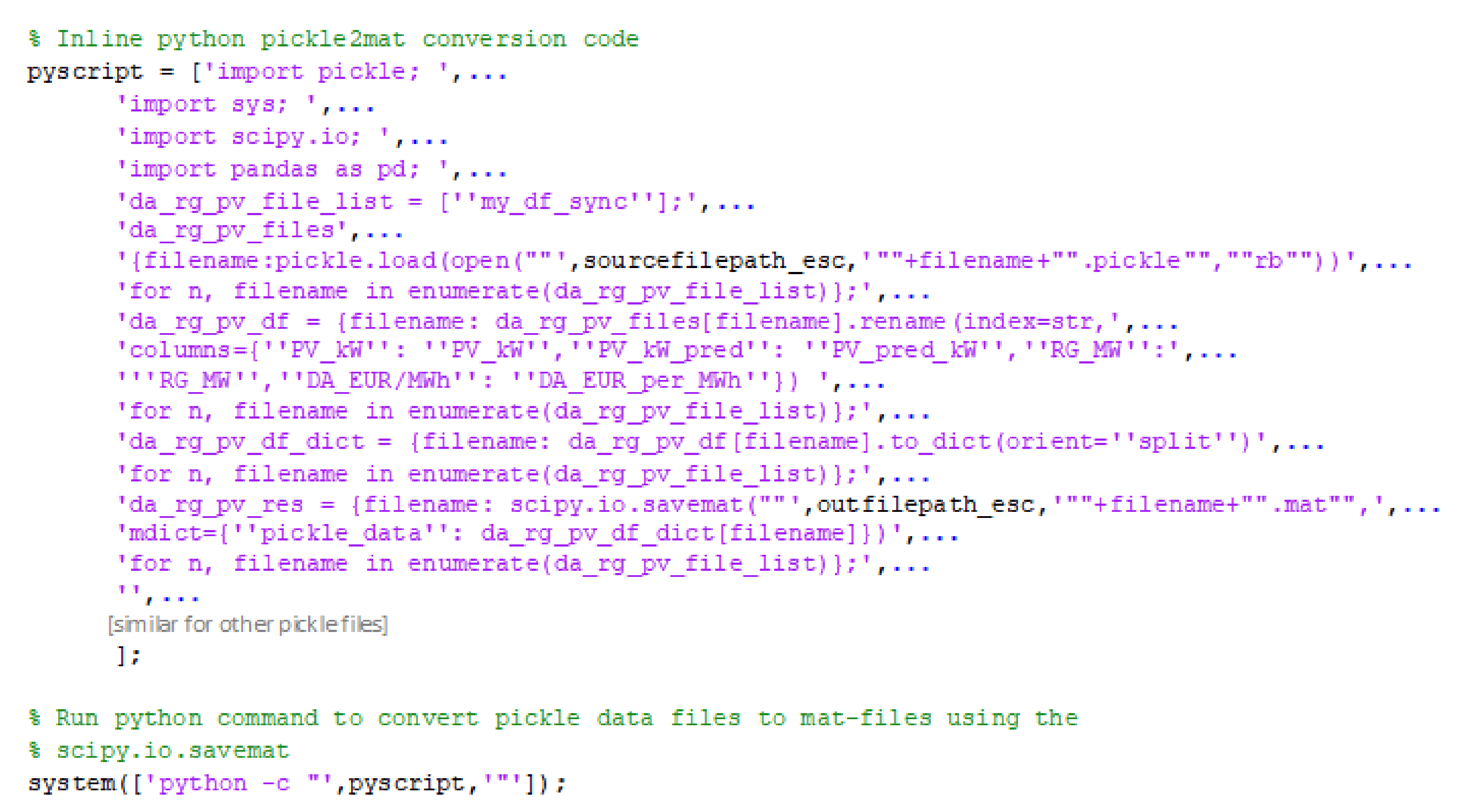
Appendix A. Data Preparation

MATLAB/Simulink [48] is used to simulate the data. Therefore, the given datasets have to be converted from the Python-specific “pickle” format to a MATLAB readable data format, where the “.mat” format has been chosen. Additionally, a prediction is made for the day-ahead electrical load and PV power values. The complete data conversion and load prediction calculation is shown in Figure A1, separated in part one Pickle2Mat and second part LoadDataPrediction. MATLAB script DSM_data_preparation_agg is the main script and creates output folders, calls the data conversion function load_agg_pickle, load data prediction function load_prediction, and plots a sample day.
Figure A1. Data conversion framework (*: placeholder for all subsets).
Energies 15 01619 g0a1
In function load_agg_pickle inline Python code has been called using the scipy.io.savemat method (Figure A2). The aggregated variables are saved in a MATLAB timetable.
Figure A2. MATLAB implementation of Python source code.
Energies 15 01619 g0a2
Additional predictions of electrical day-ahead load values P L , p r e d ( t ) in Equation (A2) have been generated in function load_prediction using the same method as P P V , p r e d has been generated in the proposed data set according to Equation (A1):
P P V , p r e d ( t ) = p P P V ( t ) + ( 1 p ) P P V ( t τ d a y )
P L , p r e d ( t ) = p P L ( t ) + ( 1 p ) P L ( t τ d a y )
where τ d a y is the same time one day before, P P V ( t ) is the PV power production, and P L ( t ) is the actual load demand at time t, and p is a weighting factor of value 0.75, which was similarly used for PV power prediction in the given data set.
The following section explores the predictability of the anticipated values. Such as in Figure A3a,b, the annual pattern electrical power consumption and photovoltaic power production of the measured and predicted values are illustrated as reflected in Equations (A1) and (A2). Figure A3c shows the box plot of the error distribution between measured and predicted values of residential energy consumption on a week-day basis and on a monthly basis respectively. The median percentage error on a daily basis ranges from about 18–30%, the 25th percentile is about 14 % , and the 75th percentile between 26 % and 61 % . The maximum error is between 69– 191 % , where minimal percentage error on a daily basis is between 3 % and 10 % . On a monthly view, one can see, that in summer months, the 75th percentile is higher (48– 64 % ), than in the rest of the year (27– 34 % ) with a median percentage error between 18– 30 % . In addition, the maximum error values are higher (148– 191 % ) in summer. The heat map in Figure A3e shows that the maximum prediction error is in the morning and in the evening in both directions, underestimation and overestimation.
Prediction of photovoltaic energy production shows higher maximum error values, on a week-day basis (Figure A3d) ranging from 126– 943 % and on a monthly perspective of view between 71 % and 943 % . Whereas the median percentage error is lower (week-day: 15– 23 % , monthly: 5– 26 % ), compared to the load prediction values. Monthly 75th percentile values are between 14 % and 24 % in the summer months, April to September with a peak in June ( 51 % ) compared to 43– 95 % in the other months. The 25th percentile values in summer is between 2– 10 % , compared to rest of the year with 14– 19 % . As expected, the higher fluctuations in the prediction error outside summer time result from the corresponding fluctuations of the solar irradiation due to unstable weather conditions (cloudiness) that lead to high errors at low values as shown in Figure A3f.
Figure A3. (a) Measured and predicted values of electrical power consumption of a household, (b) PV power production, (c) relative prediction error distribution statistics of residential power consumption, and (d) pv power production, (e) corresponding absolute error values over one year for power consumption, and (f) PV power production [43].
Energies 15 01619 g0a3
Furthermore, to depict the behavior of EV (dis)charging, a Tesla Model Y Performance has been chosen as the electrical vehicle. The charging curve data has been extracted from [49], and is limited by a maximal grid demand of 20 kW for EV charging, as shown in Figure A4. As one can see, the charging behavior can be split into two sections:
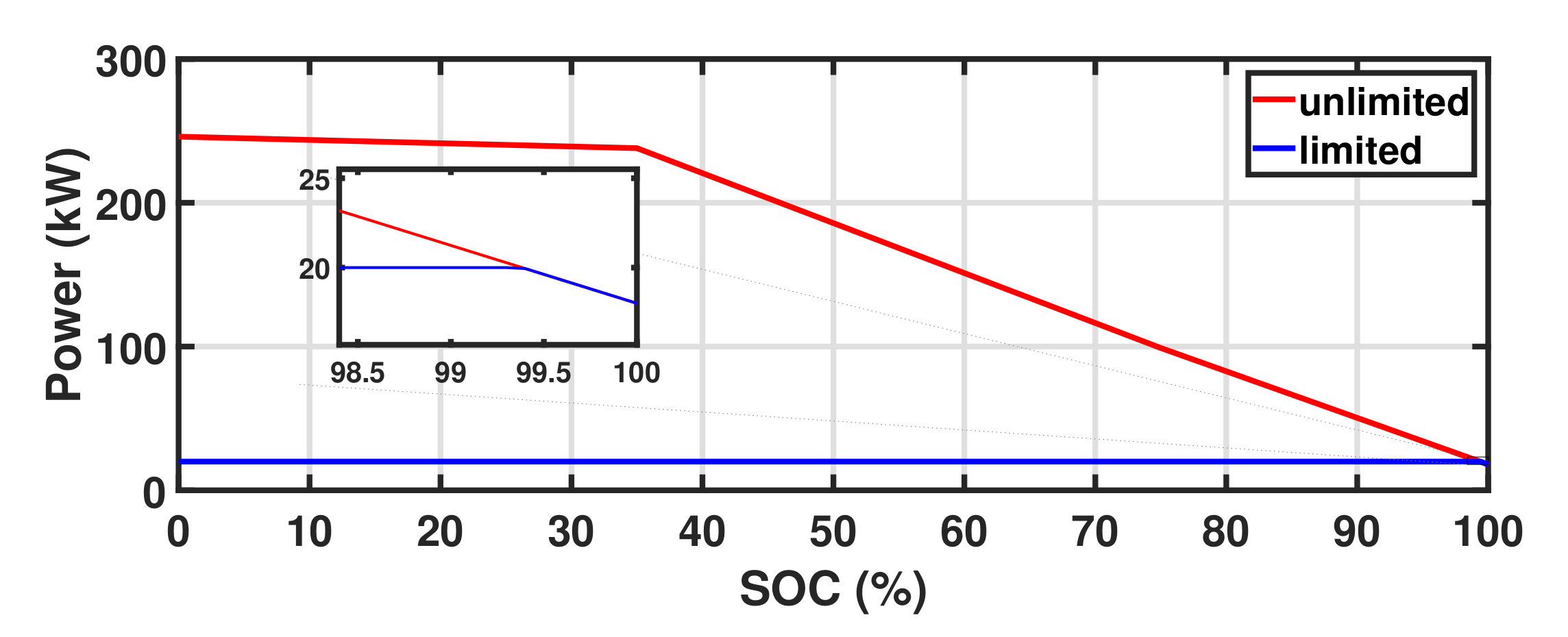
  • Fast charging between 0–35% of SOC and;
  • Decreased charging between 35–100% of SOC.
By limiting the charging power from the grid to a maximum of 20 kW, particularly for the HAPN, there is only a reduction of the charging power above 99.5% to 18 kW. This value can be higher for commercial charging ports.
Figure A4. EV charging curve of a Tesla Model Y Performance [49] limited by 20-kW grid demand power.
Energies 15 01619 g0a4

Appendix B. Battery Degradation Model

The capacity loss due to the solid electrolyte interface (SEI) layer growth and active material (AM) loss at each time step t may be computed using Equations (A3) and (A4), respectively [40].
Q SEI ( t ) = t 1 t k SEI exp E SEI R T 2 ( 1 + λ θ ) t d t ,
Q AM ( t ) = t 1 t k AM exp E AM R T · SOC ( t ) · I b a t t , d i s c h ( t ) I b a t t , c h ( t ) d t ,
where k S E I , E S E I , λ , k A M , and E A M are constant parameters given in Table 3. Q S E I represents the capacity loss caused by the SEI layer in percent, Q A M represents the capacity loss caused by active material decomposition in percent. Where R is the ideal gas constant, and T represents the cell temperature. S O C is the state of charge, I b a t t , d c h is the discharging current, I b a t t , c h is the charging current, θ is a function of SOC and the current, also given in Equation (A5):
θ = exp n F R T η k + U n OCP U s OCP
where n = 2 represents the number of electrons reduced in the reaction, F represents the Faraday constant, and U s OCP represents the side reaction’s open circuit potential. η k is specified in Equation (A6), and U n OCP is the open circuit potential of the anode as determined by Equation (A8):
η k = R T α F ln ξ + ξ 2 + 1 ,
where α = 0.5 is the transfer coefficient of the electrochemical reaction, and ξ is defined by Equation (A7).
ξ = R s I 6 ε AM , 0 i 0 V .
In this equation, R s = 7.5× 10 6 is the particle radius of the active material in m, I is the ampere current, ϵ A M , 0 = 0.552 is the active material’s initial volume fraction, i 0 = 0.05 is the complexation current exchange current density in amp/m 2 , and V = 1.26× 10 5 is the anode’s total volume in m 3 [40].
U n O C P = 0.6379+ 0.5416exp ( 305.5309z ) + 0.044tanh z 0.1958 0.1088 0.1978tanh z 1.0571 0.0854 0.6875tanh z + 0.0117 0.0529 0.0175tanh z 0.5692 0.0875 ,
where z = C Li C Li . max . The concentration of lithium ions at the graphite particle interface is denoted by C Li , and the highest lithium concentration in the graphite electrode is denoted by C Li . max [40]. Besides, z and S O C are related as z = SOC · z 100 % z 0 % + z 0 % , where z 100 % = 0.9 and z 0 % = 0 .

References

  1. U.S. Energy Information Administration. An Assessment of Energy Technologies and Research Opportunities. In Energy Inf. Adm.; 2020. Available online: www.eia.gov/tools/faqs/faq.php?id=86&t=1 (accessed on 15 January 2022).
  2. Javaid, N.; Hafeez, G.; Iqbal, S.; Alrajeh, N.; Alabed, M.S.; Guizani, M. Energy Efficient Integration of Renewable Energy Sources in the Smart Grid for Demand Side Management. IEEE Access 2018, 6, 77077–77096. [Google Scholar] [CrossRef]
  3. Ryu, K.S.; Kim, D.J.; Ko, H.; Boo, C.J.; Kim, J.; Jin, Y.G.; Kim, H.C. MPC Based Energy Management System for Hosting Capacity of PVs and Customer Load with EV in Stand-Alone Microgrids. Energies 2021, 14, 4041. [Google Scholar] [CrossRef]
  4. Li, T.; Dong, M. Residential Energy Storage Management With Bidirectional Energy Control. IEEE Trans. Smart Grid 2019, 10, 3596–3611. [Google Scholar] [CrossRef] [Green Version]
  5. Burmester, D.; Rayudu, R.; Seah, W.; Akinyele, D. A review of nanogrid topologies and technologies. Renew. Sustain. Energy Rev. 2017, 67, 760–775. [Google Scholar] [CrossRef]
  6. Minhas, D.M.; Frey, G. Rolling Horizon Based Time-Triggered Distributed Control for AC/DC Home Area Power Network. IEEE Trans. Ind. Appl. 2021, 57, 4021–4032. [Google Scholar] [CrossRef]
  7. Betancur, D.; Duarte, L.F.; Revollo, J.; Restrepo, C.; Díez, A.E.; Isaac, I.A.; López, G.J.; González, J.W. Methodology to Evaluate the Impact of Electric Vehicles on Electrical Networks Using Monte Carlo. Energies 2021, 14, 1300. [Google Scholar] [CrossRef]
  8. Elmeligy, M.M.; Shaaban, M.F.; Azab, A.; Azzouz, M.A.; Mokhtar, M. A Mobile Energy Storage Unit Serving Multiple EV Charging Stations. Energies 2021, 14, 2969. [Google Scholar] [CrossRef]
  9. Yoo, Y.; Al-Shawesh, Y.; Tchagang, A. Coordinated Control Strategy and Validation of Vehicle-to-Grid for Frequency Control. Energies 2021, 14, 2530. [Google Scholar] [CrossRef]
  10. Minhas, D.M.; Frey, G. Modeling and Optimizing Energy Supply and Demand in Home Area Power Network (HAPN). IEEE Access 2020, 8, 2052–2072. [Google Scholar] [CrossRef]
  11. Ran, X.; Leng, S. Enhanced Robust Index Model for Load Scheduling of a Home Energy Local Network With a Load Shifting Strategy. IEEE Access 2019, 7, 19943–19953. [Google Scholar] [CrossRef]
  12. Ali, A.Y.; Hussain, A.; Baek, J.W.; Kim, H.M. Optimal Operation of Networked Microgrids for Enhancing Resilience Using Mobile Electric Vehicles. Energies 2021, 14, 142. [Google Scholar] [CrossRef]
  13. Liao, J.T.; Huang, H.W.; Yang, H.T.; Li, D. Decentralized V2G/G2V Scheduling of EV Charging Stations by Considering the Conversion Efficiency of Bidirectional Chargers. Energies 2021, 14, 962. [Google Scholar] [CrossRef]
  14. Ustun, T.S.; Hussain, S.M.S.; Kikusato, H. IEC 61850-Based Communication Modeling of EV Charge-Discharge Management for Maximum PV Generation. IEEE Access 2019, 7, 4219–4231. [Google Scholar] [CrossRef]
  15. Abdalla, M.A.A.; Min, W.; Mohammed, O.A.A. Two-Stage Energy Management Strategy of EV and PV Integrated Smart Home to Minimize Electricity Cost and Flatten Power Load Profile. Energies 2020, 13, 6387. [Google Scholar] [CrossRef]
  16. Wu, J.; Wei, Z.; Li, W.; Wang, Y.; Li, Y.; Sauer, D.U. Battery Thermal- and Health-Constrained Energy Management for Hybrid Electric Bus Based on Soft Actor-Critic DRL Algorithm. IEEE Trans. Ind. Inform. 2021, 17, 3751–3761. [Google Scholar] [CrossRef]
  17. Zeiselmair, A.; Köppl, S. Constrained Optimization as the Allocation Method in Local Flexibility Markets. Energies 2021, 14, 3932. [Google Scholar] [CrossRef]
  18. Khan, S.U.; Mehmood, K.K.; Haider, Z.M.; Rafique, M.K.; Khan, M.O.; Kim, C.H. Coordination of Multiple Electric Vehicle Aggregators for Peak Shaving and Valley Filling in Distribution Feeders. Energies 2021, 14, 352. [Google Scholar] [CrossRef]
  19. Nishimwe H., H.L.F.; Yoon, S.-G. Combined Optimal Planning and Operation of a Fast EV-Charging Station Integrated with Solar PV and ESS. Energies 2021, 14, 3152. [Google Scholar] [CrossRef]
  20. Alrumayh, O.; Bhattacharya, K. Flexibility of Residential Loads for Demand Response Provisions in Smart Grid. IEEE Trans. Smart Grid 2019, 10, 6284–6297. [Google Scholar] [CrossRef]
  21. Zhou, L.; Zhang, Y.; Lin, X.; Li, C.; Cai, Z.; Yang, P. Optimal Sizing of PV and BESS for a Smart Household Considering Different Price Mechanisms. IEEE Access 2018, 6, 41050–41059. [Google Scholar] [CrossRef]
  22. Ouramdane, O.; Elbouchikhi, E.; Amirat, Y.; Sedgh Gooya, E. Optimal Sizing and Energy Management of Microgrids with Vehicle-to-Grid Technology: A Critical Review and Future Trends. Energies 2021, 14, 4166. [Google Scholar] [CrossRef]
  23. Salvatti, G.A.; Carati, E.G.; Cardoso, R.; da Costa, J.P.; Stein, C.M.d.O. Electric Vehicles Energy Management with V2G/G2V Multifactor Optimization of Smart Grids. Energies 2020, 13, 1191. [Google Scholar] [CrossRef] [Green Version]
  24. Yu, L.; Jiang, T.; Zou, Y. Online Energy Management for a Sustainable Smart Home With an HVAC Load and Random Occupancy. IEEE Trans. Smart Grid 2019, 10, 1646–1659. [Google Scholar] [CrossRef] [Green Version]
  25. Moon, S.; Lee, J. Multi-Residential Demand Response Scheduling With Multi-Class Appliances in Smart Grid. IEEE Trans. Smart Grid 2018, 9, 2518–2528. [Google Scholar] [CrossRef]
  26. Shahab, M.; Wang, S.; Junejo, A.K. Improved Control Strategy for Three-Phase Microgrid Management with Electric Vehicles Using Multi Objective Optimization Algorithm. Energies 2021, 14, 1146. [Google Scholar] [CrossRef]
  27. Von Bonin, M.; Dörre, E.; Al-Khzouz, H.; Braun, M.; Zhou, X. Impact of Dynamic Electricity Tariff and Home PV System Incentives on Electric Vehicle Charging Behavior: Study on Potential Grid Implications and Economic Effects for Households. Energies 2022, 15, 1079. [Google Scholar] [CrossRef]
  28. Al-Quraan, A.; Al-Qaisi, M. Modelling, Design and Control of a Standalone Hybrid PV-Wind Micro-Grid System. Energies 2021, 14, 4849. [Google Scholar] [CrossRef]
  29. Wang, L.; Wu, Z.; Cao, C. Integrated Optimization of Routing and Energy Management for Electric Vehicles in Delivery Scheduling. Energies 2021, 14, 1762. [Google Scholar] [CrossRef]
  30. Minhas, D.M.; Frey, G. Two-Stage Multi-time Scale Energy Management Control framework for Home Area Power Network. In Proceedings of the 2020 IEEE International Conference on Environment and Electrical Engineering and 2020 IEEE Industrial and Commercial Power Systems Europe (EEEIC/I CPS Europe), Madrid, Spain, 9–12 June 2020; pp. 1–6. [Google Scholar] [CrossRef]
  31. Zhang, Q.; Zhao, J.; Wang, X.; Tong, L.; Jiang, H.; Zhou, J. Distribution Network Hierarchically Partitioned Optimization Considering Electric Vehicle Orderly Charging with Isolated Bidirectional DC-DC Converter Optimal Efficiency Model. Energies 2021, 14, 1614. [Google Scholar] [CrossRef]
  32. Minhas, D.M.; Frey, G. Optimal Scheduling of Energy Supply Entities in Home Area Power Network. In Proceedings of the 2019 6th International Conference on Control, Decision and Information Technologies (CoDIT), Paris, France, 23–26 April 2019; pp. 732–737. [Google Scholar] [CrossRef]
  33. Trinh, P.H.; Chung, I.Y. Optimal Control Strategy for Distributed Energy Resources in a DC Microgrid for Energy Cost Reduction and Voltage Regulation. Energies 2021, 14, 992. [Google Scholar] [CrossRef]
  34. Wu, J.; Wei, Z.; Liu, K.; Quan, Z.; Li, Y. Battery-Involved Energy Management for Hybrid Electric Bus Based on Expert-Assistance Deep Deterministic Policy Gradient Algorithm. IEEE Trans. Veh. Technol. 2020, 69, 12786–12796. [Google Scholar] [CrossRef]
  35. Savard, C.; Iakovleva, E.; Ivanchenko, D.; Rassõlkin, A. Accessible Battery Model with Aging Dependency. Energies 2021, 14, 3493. [Google Scholar] [CrossRef]
  36. Zhu, Y.; Zhao, D.; Li, X.; Wang, D. Control-Limited Adaptive Dynamic Programming for Multi-Battery Energy Storage Systems. IEEE Trans. Smart Grid 2019, 10, 4235–4244. [Google Scholar] [CrossRef]
  37. Hao, H.; Wu, D.; Lian, J.; Yang, T. Optimal Coordination of Building Loads and Energy Storage for Power Grid and End User Services. IEEE Trans. Smart Grid 2018, 9, 4335–4345. [Google Scholar] [CrossRef]
  38. Hu, J.; He, H.; Wei, Z.; Li, Y. Disturbance-Immune and Aging-Robust Internal Short Circuit Diagnostic for Lithium-Ion Battery. IEEE Trans. Ind. Electron. 2022, 69, 1988–1999. [Google Scholar] [CrossRef]
  39. Wikner, E.; Thiringer, T. Extending battery lifetime by avoiding high SOC. Appl. Sci. 2018, 8, 1825. [Google Scholar] [CrossRef] [Green Version]
  40. Jin, X.; Vora, A.; Hoshing, V.; Saha, T.; Shaver, G.; García, R.E.; Wasynczuk, O.; Varigonda, S. Physically-based reduced-order capacity loss model for graphite anodes in Li-ion battery cells. J. Power Sources 2017, 342, 750–761. [Google Scholar] [CrossRef] [Green Version]
  41. Neon Neue Energieökonomik GmbH. Open Power System Data. 2021. Available online: https://data.open-power-system-data.org/time_series/ (accessed on 18 February 2021).
  42. Feldman, D.; Ramasamy, V.; Fu, R.; Ramdas, A.; Desai, J.; Margolis, R. U.S. Solar Photovoltaic Systemand Energy Storage CostBenchmark: Q1 2020; National Renewable Energy Lab. (NREL): Golden, CO, USA, 2020. [Google Scholar]
  43. Rheinberger, K.; DSM-Data. GitHub Repository. 2021. Available online: https://github.com/klaus-rheinberger/DSM-data (accessed on 18 February 2021).
  44. ENTSO-E. Transparency Platform. 2021. Available online: https://transparency.entsoe.eu/ (accessed on 18 February 2021).
  45. European Commission, Joint Research Centre. PVGIS—Photovoltaic Geographical Information System. 2021. Available online: https://re.jrc.ec.europa.eu/pvg_tools/en/tools.html (accessed on 18 February 2021).
  46. EA Technology. My Electric Avenue. 2021. Available online: https://eatechnology.com/americas/resources/projects/my-electric-avenue-data-download/ (accessed on 18 February 2021).
  47. Commission for Energy Regulation. CER Smart Metering Project-Electricity Customer Behaviour Trial, 2009–2010, 1st Edition, Irish Social Science Data Archive, SN: 0012-00. 2021. Available online: https://www.ucd.ie/issda/data/commissionforenergyregulationcer/ (accessed on 18 February 2021).
  48. MATLAB. Version 9.9 (R2020b); The MathWorks Inc.: Natick, MA, USA, 2020. [Google Scholar]
  49. Hösl, N.; Teulings, T. Open EV Data. 2021. Available online: https://github.com/chargeprice/open-ev-data (accessed on 18 February 2021).
Figure 1. Proposed iEMS framework.
Energies 15 01619 g001
Figure 2. HAPN architecture.
Energies 15 01619 g002
Figure 3. Flowchart of the conventional rule-based scheduling scheme (Conv-EG).
Energies 15 01619 g003
Figure 4. Flowchart of the conventional rule-based scheduling scheme (Conv-PEG).
Energies 15 01619 g004
Figure 5. Flowchart of the proposed scheduling scheme (MP-iEMS).
Energies 15 01619 g005
Figure 6. Case I flow chart.
Energies 15 01619 g006
Figure 7. Case II flow chart.
Energies 15 01619 g007
Figure 8. Case III flow chart.
Energies 15 01619 g008
Figure 9. Case IV flow chart.
Energies 15 01619 g009
Figure 10. Case V flow chart.
Energies 15 01619 g010
Figure 11. Case VI flow chart.
Energies 15 01619 g011
Figure 12. Grid energy price signal.
Energies 15 01619 g012
Figure 13. Comparative power utilization.
Energies 15 01619 g013
Figure 14. Total energy cost.
Energies 15 01619 g014
Figure 15. Total grid energy cost.
Energies 15 01619 g015
Figure 16. Total EV storage utilization cost.
Energies 15 01619 g016
Figure 17. Histogram of EV storage SOC.
Energies 15 01619 g017
Figure 18. Histogram of EV storage charge rates.
Energies 15 01619 g018
Figure 19. Annual accumulative charge and discharge energy for EV storage.
Energies 15 01619 g019
Figure 20. Total EV storage loss.
Energies 15 01619 g020
Figure 21. Comparison of total capacity loss.
Energies 15 01619 g021
Figure 22. Comparison of various capacity losses among different schemes.
Energies 15 01619 g022
Figure 23. Hourly mean total loss increment for Scheme 1 (Conv-EG).
Energies 15 01619 g023
Figure 24. Hourly mean total loss increment for Scheme 2 (Conv-PEG).
Energies 15 01619 g024
Figure 25. Hourly mean total loss increment for Scheme 3 (MP-iEMS).
Energies 15 01619 g025
Table 1. Objectives, limitations, and critical analysis of the past literature.
Ref #.ObjectivesTechnique(s)Scheduling EntitiesDynamic EV
Charging
Battery
Degradation
Cost
Reduction
Energy
Balancing
Limitation(s)
GridPVEV
[3]According to this study, using battery storage for PV and
EV hosting capacity optimization as well as grid voltage
maintenance was critical.
Model Predictive
Control
The case study is fictitious. It was confirmed that the
generation of DG and PVs exceeds the consumption
of the load and EV charging and that the ESS
maintains all bus voltages within the permitted limit.
[22]The purpose of this study is to propose a methodology
for simulating plug-in electric vehicle charging in order
to quantify the impact of this type of load on
power systems.
Monte Carlo
Simulation
The proposed technique focused on transmission
networks and provides a deterministic representation
of the EV charge distribution across the network.
It made no reference to any real-world data collection.
[23]Dynamic programming is used to govern the charging (G2V)
and discharging of the storage device (V2G) in order to extend
the life of the battery and minimizing grid reliance.
Adaptive Dynamic
Programming
The model was confined to battery storage alone and
did not include specific information about load
needs. Additionally, constraint functions that do not
have an exact model of the device were estimated.
[24]The author discussed the challenge of minimizing the total of
energy and thermal discomfort costs. The suggested system
stabilized developing queues for indoor temperature
control, electric car charging, and energy storage.
Lyapunov
Optimization
The energy demand model was limited in scope since
it examines only thermal loads. Additionally, the
algorithm was incapable of addressing the issue of
peak forms.
[25]Maximizing the utility sums of residential customers while
keeping energy consumption costs in check is explored in
this article. It is decentralized, but it protected the
residents’ private information at the same time.
Generalized Benders
Decomposition algorithm
The technique might not operate successfully
if the homes’ demand information is inaccurate.
It also did not address the peak-to-average
power demand ratio (PAR).
[20]A two-stage optimization approach is devised, in which
peak reduction signals are discovered and their flexibility
provision determined by aggregating individual users’
energy use histories.
Mixed Integer Linear
Programming
This study made no allowance for incentives for
postponing loading or for the penalty cost
associated with reducing customer suffering.
[26]The control method outlined in this work is intended
to address power factor concerns associated with
EV charging stations while still allowing
for full PV generation.
Optimal Dynamic
Programming
The effort was done to boost the power factor.
The battery management system was designed to
adjust only the power factor, ignoring the demand-
supply balance and ignoring real-world data.
[27]This study examines the influence of dynamic energy
pricing and home PV system incentives on EV
charging behavior, grid load, and household economics.
Mixed Integter Linear
Programming
The battery deterioration model outlined in this
study is critical to the model’s success. Realistic
information about the actions of prosumers
was also not included.
[15]The suggested technique uses time-of-use pricing,
time-varying residential power demand, solar generating
profiles, and EV specifications to reduce electricity
prices and flatten the load curve.
Rule Based
Optimization
The battery degradation model is an important
factor in this study’s model. However,
realistic data sets on prosumer
actions were not included in the investigation.
[28]The PV produced more energy than needed to meet load
demands and charge the batteries. Battery discharge
happens when PV panel output falls short of
load needs. The controller prevented over(dis)charging.
Fuzzy Logic
Design
The focus of this paper was solely on the
supply and demand for energy. Cost reduction
and customer satisfaction were not
adequately addressed.
Table 2. System parameters.
ParametersValueParametersValueParametersValue
P g . d i s p 20 kW η b . c o n 0.98 t 15 min
E b , 0 110 kWh η p v . c o n 0.98 k 1 s
E ¯ b 120 kWh ϕ [42]130 $/MWh P ¯ b . c h Figure A4
E ̲ b 1 kWh φ [42]201 $/MWh P ¯ b . d c h Figure A4
Table 3. Coefficients of the simplified reduced-order model.
ParametersValueUnitParametersValueUnit
k S E I 6684.8 1 s E S E I 39,146J/mol
k A M 1.3681/Ah E A M 39,500J/mol
R8.314J/K·mol λ 5.5× 10 5 -
F96,485.3C/mol U s OCP 0.4 -
Table 4. Comparison of ESEs utilization factor (UF) and penetration level (PL) for various schemes.
Scheme/Parameters K PV . UF K G . UF K EV . UF K PV . PL K G . PL K EV . PL K SS
Scheme 1: (Conv-EG)00.03070.959700.85980.41980.1402
Scheme 2: (Conv-PEG)0.66340.02680.95980.11290.76390.40980.2361
Scheme 3: (MP-iEMS)0.62720.02690.95790.11750.84470.35330.1553
Publisher’s Note: MDPI stays neutral with regard to jurisdictional claims in published maps and institutional affiliations.

