Abstract
Operation of distribution networks involves a series of criteria that should be met, aiming for the correct and optimal behavior of such systems. Some of the major drawbacks found when studying these networks is the real losses related to them. To overcome this problem, distribution network reconfiguration (DNR) is an efficient tool due to the low costs involved in its implementation. The majority of studies regarding this subject treat the problem by considering networks only as three-phase balanced, modeled as single-phase grids with fixed power demand, which is far from representing the characteristics of real networks (e.g., unbalanced loads, variable power and unbalance indexes). Due to the combinatorial nature of the problem, metaheuristic techniques are powerful tools for the inclusion of such characteristics. In this sense, this paper proposes a study of DNR considering balanced and unbalanced systems with variable power demand. An analysis of the direct influence of voltage unbalance index (VUI) and current unbalance index (CUI) is carried out for unbalanced cases. To solve the DNR problem, a selective bio-inspired metaheuristic based on micro bats’ behavior named the selective bat algorithm (SBAT) is used together with the EPRI-OpenDSS software (California, US, EPRI). Tests are initially conducted on balanced systems, aiming to validate the technique proposed for both demands and state their differences, and then they are conducted on unbalanced systems to study the influence of VUI and CUI in the DNR solution.
1. Introduction
1.1. Motivation and Incitement
Distribution systems are the final third of electric power systems’ traditional structure of generation, transmission and distribution, being responsible for delivering energy to consumers and needing reliable operation. When considering the medium voltage primary distribution networks, one of the main concerns is related to real losses through lines.
To treat and reduce these impacts, a number of solutions can be applied, such as: changing the infrastructure of the network (e.g., installing distributed generation in specific points), which may be financially or physically infeasible, or modifying the topology of the system through the operation of disconnect switches [1]. This second option, namely, distribution network reconfiguration (DNR), ends up being the most favorable due to the low costs involved in its implementation and the effective results achieved, not only reducing losses through lines but also improving the voltage limits.
Due to the combinatorial nature of the problem, determined by the relation, where n is the number of switches that may or not be open, and its characteristic of a mixed integer nonlinear problem (MINLP), deterministic approaches become practically unfeasible. Hence, to solve the problem, heuristics and metaheuristics are often used, as, although not guaranteeing finding the global optimum, they present good solutions and are almost straightforward when applied to optimization problems, as opposed to numerical and mathematical methods that may increase the difficulty of modeling the studied problem [2]. This tendency is seen in studies presented for the solution of the DNR problem in the last 30 years [2].
Although advances in the techniques to solve the DNR problem have been presented throughout the years, the majority of papers consider all networks as three-phase balanced, without taking into consideration particularities of real distribution systems, such as load unbalancing, voltage and current unbalance indexes and variable demand. Based on these arguments, the paper presented here aims to cover all these matters, proposing to model the network as three-phase unbalanced with variable demand and considering the influence of the voltage and current unbalance indexes in the DNR solution. The solution is provided through a bio-inspired metaheuristic.
1.2. Literature Review
The conventional DNR methods consider a simplified approximation of the system, in which a balanced three-phase grid is modeled as a single-phase grid with fixed power demand. This approach has been applied since the 1970s, with [3] as the pioneer study on the subject. In [3], the authors used a deterministic and a heuristic method to solve the problem. The same model continued to be used in the years following [4,5,6]. In most of these studies, alterations occur only in the method used to solve the problem. In [6], the authors presented a genetic algorithm (GA)-based technique to reduce losses in two systems. In [5], the authors presented techniques based on neural networks aiming at losses reduction, while in [4], a simulated annealing technique is applied to reduce losses on three different systems.
Until today, most studies were based on models similar to the approximations used in earlier studies; nevertheless, new heuristics, metaheuristics and especially bio-inspired methods have been continuously proposed throughout the years in order to improve the solutions found to the DNR problem. In [7], the authors presented an ant colony optimization (ACO) algorithm to reduce losses on 16- and 84-bus systems. In [8], the authors proposed a new heuristic based on the direction of power flow to solve the DNR problem, aimed at losses reduction on 33-, 69- and 84-bus systems. The authors of [9] proposed three different approaches in the following years. The first approach [9] is based on particle swarm optimization (PSO) and was applied by the authors to reduce losses on 33- and 69-bus systems, the second [10] uses a modified tabu-search algorithm (TSA) to reduce losses on 16-, 69- and 119-bus systems with three load levels (light, normal and heavy), and, in the third paper [11], the authors proposed the use of the ACO and harmony search (HS) algorithm to reduce losses on 33- and 119-bus systems. In the following years, the authors in [12] presented an algorithm based on bacterial foraging (BFA) to reduce losses on 16-, 33- and 69-bus systems. In the same year as [12], authors in [13] presented an approach to solve the DNR problem aimed at losses reduction using the cuckoo search algorithm (CSA) and applied it on 33-, 69- and 119-bus systems. Subsequently, two new approaches were presented by the authors of [13], one based again on the CSA [14] to allocate DG alongside DNR, applying it to 33-, 69- and 119-bus systems, and a second paper based on the runner root algorithm (RRA) [15], applied to a multiobjective DNR on 33- and 69-bus systems.
More recently, the authors in [16] presented an approach based on selective particle swarm optimization (SPSO) to reduce losses on 33- and 84-bus systems, discussing variations of the SPSO to solve the problem. In [17], a customized evolutionary algorithm is proposed to solve the DNR problem, where the objective is to reduce a fitness function that considers power losses and voltage profile on 33-, 69- and 119-bus systems. In [18], the authors presented a discrete PSO to reduce voltage fluctuations on a 69-bus system and on a practical 95-bus system. In [19], a discussion of three heuristic methods to solve the DNR problem, aiming to reduce total harmonic distortion (THD) on 69- and 119-bus systems, is presented, while in [20,21], respectively, an improved sine–cosine algorithm to both reconfigure the system and allocate DG units on 33- and 69-bus systems and an approach based in GA and PSO to improve the system reliability on a 33-bus system are presented.
In past years, some works took into account a variable power demand but still considered the system three-phase balanced, as seen in [22,23] and more recently in [24,25].
Although DNR methods based on bio-inspired and metaheuristic techniques have been continuously proposed, as well as some papers considering variable demand, some crucial aspects of distribution networks have not been taken into account, such as characteristics related to unbalanced systems.
One of the first studies on the subject was presented by [26] in the beginning of the 1990s. In the following years, a reduced number of papers raised this approach, such as [27,28]. In recent years, the subject came into more prominence, as seen in [29,30]. Through brief bibliographical research, the reduced number of papers presenting the DNR under such conditions in comparison with the traditional model (balanced with fixed demand) is clearly noticed. In addition, the majority of studies were carried out considering the power demand fixed, i.e., without load variations over time. Some examples that present unbalanced systems with variable demand are [31,32,33,34,35]. In [31,32], the DNR problem for unbalanced systems is solved through a heuristic approach, while in [33,34,35], the authors applied, respectively, a heuristic together with GA [33], GA [34] and TSA, together with a harper search sphere (HSS) [35]. In the majority of cases, although dealing with unbalanced networks, unbalance indexes are not taken into consideration, with only some papers dealing with this aspect, for example [29,36]. However, the influence of these indexes, which may be important in some specific cases [37,38], and how they can directly affect solutions found, depending on limits established, is not the direct focus of these papers.
1.3. Main Contributions and Structure
In this context, this research proposes to model the DNR problem considering first balanced systems and then unbalanced distribution systems under the influence of VUI and CUI, both with fixed and variable power demand. The consideration of these two cases (fixed and variable) helps to illustrate the differences between both approaches, starting from the objective function and going through the results presented, which might be different between them.
High levels of VUI can affect losses, operation of polyphase electric machines, three-phase power electronic loads [37] and high levels of CUI can cause difficulties related to ground fault protection relay [37] and influence power and energy losses [38]. Therefore, the inclusion and analysis of the influence of these indexes are the major contributions of the paper, especially considering the context of variable demand, as these are often not taken into consideration and directly affect the results of the DNR problem on unbalanced systems. The problem is solved using a variation of a bat-inspired algorithm, named the selective bat algorithm (SBAT). The main advantages of this technique are its flexible structure and consolidated theory, leading to suitable applications in a vast number of problems, providing a balance between results and computational time in comparison with deterministic techniques, and great flexibility in its structure, showing itself as more versatile than the traditional algorithms, as it can combine characteristics from PSO and HS [39]. EPRI-OpenDSS is selected to conduct the electrical analysis of the studied systems and the influence of VUI and CUI is presented in detail for the unbalanced systems.
The paper is structured as follows: Section 2 introduces the mathematical model of the problem, Section 3 presents the proposed SBAT technique, Section 4 brings the implementation and application of the proposed metaheuristic to DNR, Section 5 presents the results found and discussions regarding the influence of VUI and CUI, and, finally, Section 6 concludes the study.
2. Distribution Network Reconfiguration Mathematical Model
The DNR problem is modeled by two distinct objective functions to be minimized, one for fixed demand (reducing real losses) and other for variable demand (reducing the daily real losses costs), aiming to illustrate the differences between both. The objective functions are modeled as Equations (1) and (2) (for both balanced and unbalanced systems). The two optimization problems are subject to constraints (3)–(9). Constraints (10) and (11) are related to unbalanced cases only (fixed or variable). This model is based on the one found in [22] for balanced networks, corroborated by the one found in [40] for unbalanced networks in the presence of photo-voltaic generators (PV) and energy storage. Here, the main difference resides in considering constraints related to voltage and current unbalance indexes.
subject to:
where we use the following definitions: : conductance of branch of phase ; : set of branches of the studied system at phase ; : state of the switch at branch ; : voltage of bus i and phase ; : voltage of bus j and phase ; : angular difference of buses i and j at phase ; : set of all demand levels d; : losses costs of demand level d; : duration of demand level d; : voltage of bus i and phase at demand level d; : voltage of bus j and phase at demand level d; : angular difference of buses i and j at phase and demand level d; set of system buses connected to bus i; : active power supplied from substation to bus i at demand level d and phase ; : active power demanded by bus i at demand level d and phase ; : active power flow at branch at demand level d and phase ; : reactive power supplied from substation to bus i at demand level d and phase ; : reactive power demanded by bus i at demand level d and phase ; : reactive power flow at branch at demand level d and phase ; : minimum voltage limit; : maximum voltage limit; : total number of branches that compose the studied system; : incidence matrix of the studied system; : real component of flowing current of branch at demand level d and phase ; : imaginary component of flowing current of branch at demand level d and phase ; : total current of branch at demand level d and phase ; : admissible phase voltage imbalance index (%); : vector of voltages of all three phases at bus i and demand level d; : average voltage magnitude of all three phases at bus i and demand level d; : admissible current imbalance index (%); : vector of currents of all three phases at branch and demand level d; average current magnitude of all three phases at branch and demand level d.
Equations (3) to (7) are responsible for the following constraints: Equation (3) is the active value of the power balance. Equation (4) is the reactive value of the power balance. Equation (5) represents the minimum and maximum voltage limits, established by regulatory bodies. Equation (6) indicates the state of the system switches (open = 0, closed = 1). Equation (7) indicates the total number of switches composing a system to assure its radial operation (after DNR). Equation (8) is an additional constraint related to the radial operation, presenting a value equal to 1 or −1 when the system is in this condition [9]. Equation (9) is related to current capacity in the system branches. This last constraint can be neglected in the majority of DNR studies dealing with system losses, as its values tend to reduce together with the objective function, i.e., losses [23]. It is also worth pointing out that, as the substation capacity is neglected, substations can be concentrated in a single bus [23]. Equations (10) and (11) are constraints related to the voltage unbalance index (VUI) and current unbalance index (CUI) [41], taken into consideration only in unbalanced cases (fixed and variable).
For the cases herein studied that are three-phase and unbalanced, the objective functions are calculated by phase. The load flow is determined via EPRI-OpenDSS, allowing a simple approach to analyze the systems’ behavior under the established conditions.
The method used by EPRI-OpenDSS is based on an iterative calculation and on a method called “Normal” by the developers [42], which uses primitive admittance to determine the load flow. The details and description of the available methods in EPRI-OpenDSS are found in [42].
3. Bat Echolocation Algorithm—Selective Approach
The bat algorithm was proposed by [43], inspired by the behavior of micro bats in search of a better position to attack potential prey and avoid obstacles. Micro bats emit a high-level pulse and also listen to the reverberation of echoes coming from objects in their surroundings. Properties of the emitted pulses are correlated with the animal’s hunting strategies and can detect distance, orientation, type and velocity of a potential target [44].
Three fundamental characteristics represent the behavior, serving as the foundations of the technique according to [44]:
- Echolocation is used by all bats to perceive distance and differentiate prey from barriers;
- These same bats fly in a random way, considering the following parameters: speed and position (where i is the i-th particle), fixed minimum frequency , variable and initial loudness . The emitted pulses and pulse emission are adjustable depending on the target proximity;
- The variation of loudness is assumed as ranging from a higher value to a minimum .
Simplifications are often adopted to the algorithm, such as: limiting the frequency range and the pulse emission rate to and , where is the upper limit in the first and 0 and 1 indicate no pulse and maximum pulse rate, respectively, in the second.
Following these definitions, the main mathematical expressions of the algorithm are summarized by Equations (12)–(14):
where is given through a random number, is the current global best and is the velocity at instant t. The value of the initial frequency is randomly taken from a uniform distribution between the frequencies . The technique has a second procedure, responsible for a local search aiming to select the best value between the current solutions. Through this step, a new solution is generated for each bat using a random walk method. Equation (15) summarizes this procedure.
where is the previous position of the bat, is a random number between a given interval and is the average loudness of all bats at instant t. The values of loudness and pulse emission r have the possibility of being updated iteratively. It is typical to consider that reduces and r increases when locating a new prey. They are given by (16) and (17), respectively.
where and are constants that attenuate the values of (16) and (17) and is the initial value of the emission rate. According to [45], it is typical to set . The initial values and are given between and , respectively, updated as solutions improve [45].
As stated earlier, the algorithm has the advantage of combining characteristics of the PSO and HS algorithms when some simplifications are adopted in the parameters and , becoming an approximation of either PSO or HS. This particularity makes the bat algorithm a more versatile option in comparison with the last two when applied to solve highly combinatorial problems such as the DNR problem [43].
To correlate the algorithm with the DNR problem, some adaptations are often performed in the original structure of the technique, as the problem deals with integer values and the technique is initially conceived to deal with real variables. Normally, as proposed in this paper, a selective approach is applied to deal with this characteristic.
The proposed SBAT uses a similar adjustment as the one presented in [46] for PSO. This is conducted considering that the positions of the particles (i.e., bats) are compressed in a series of discrete integer values through a sigmoid function, transforming each i-th position coordinate.
Equations (18) and (19) summarize this process. Equation (18) describes the sigmoid function used and Equation (19) the relation established to correlate the values of Equation (18) with the switch number.
Relation (19) indicates the element S of the given vector that will be selected based on the result found by (18). Variations of the exponent of are used to achieve a better fitting to the DNR problem. In this paper, the empirically defined exponent is used for all systems.
Hence, to solve the DNR problem using the SBAT, each particle position will represent a set of switches to be opened, where each position coordinate represents a switch selected from a given search space using Relation (19) as previously established. The number of coordinates of the bats’ positioning is the same as the number of open switches needed to maintain the system operating as a radial network, , inferred from Equation (7).
Regarding the search space, it is composed of fundamental loops (FL) that are established when considering the system as a meshed network. The total number of FL is also the same as , as one switch is chosen for each FL to compose the set of switches of the solution. For example, in the 33-bus and 37-branch system [47], , and, therefore, the system is composed of five FL and the solution of five switches. A detailed description of how this is performed can be found in [1].
4. Selective Bat Algorithm Applied to DNR
The SBAT here proposed was implemented in Python and all load flow calculations were performed via the software EPRI-OpenDSS. The interface between Python and EPRI-OpenDSS is possible through COM.
As distribution networks operate in a radial way, there must be no meshes in the system. This is assured by opening one different switch of each mesh (considering that all branches have one switch and have taken into consideration the sigmoid function of Section 3) and attending the constraints related to radiality presented in Section 2, as briefly presented in Section 3
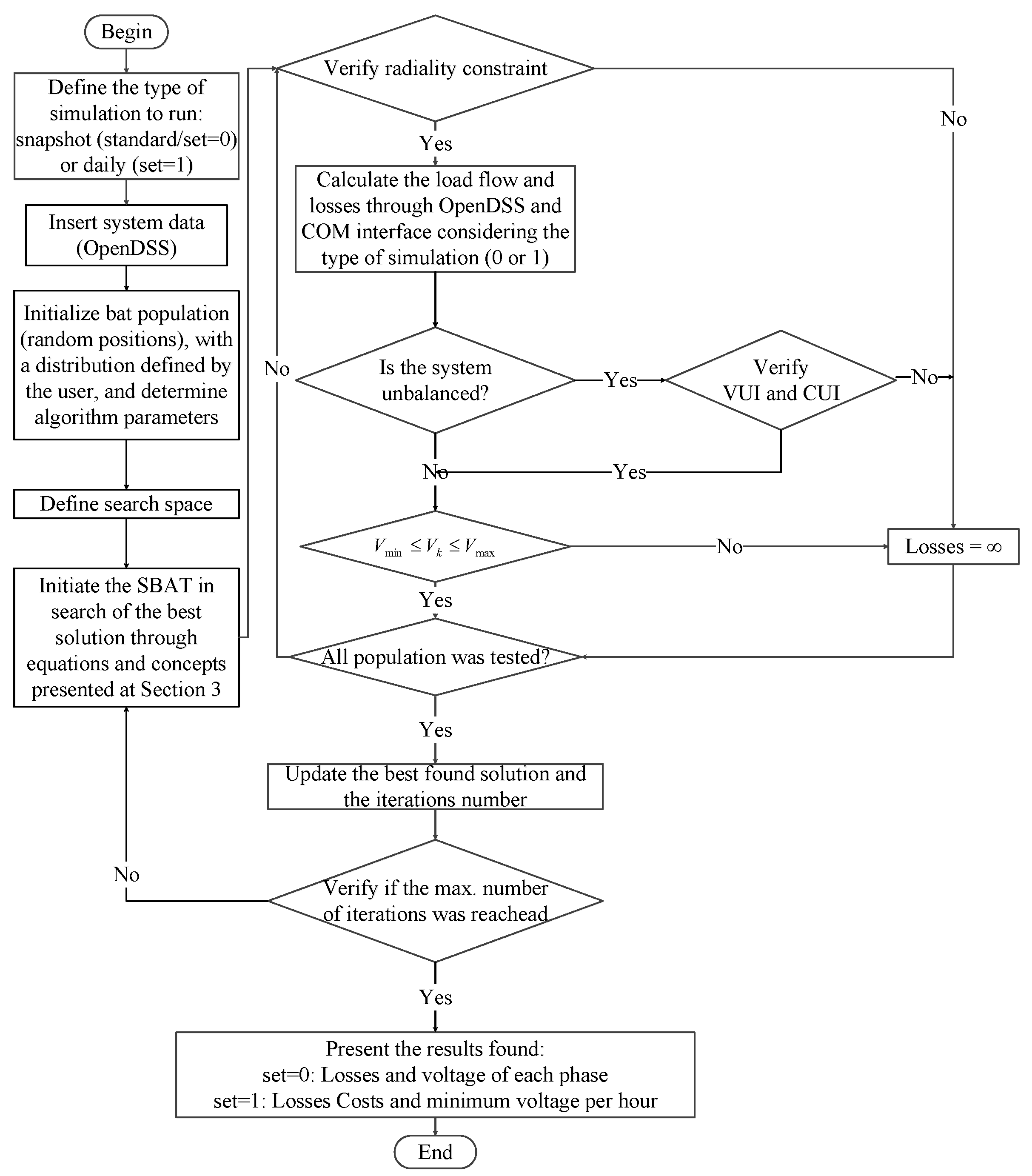
In all cases herein studied, the search process of the algorithm presented in Section 3 is directly correlated with losses (fixed demand) and total losses costs (variable demand). In summary, if a particle (bat) is near a potential prey, it indicates that the value of the objective function is better, so the remaining particles tend to walk towards this direction. In the technique, a bat represents a potential solution to the DNR problem, where its position coordinates, as previously cited, indicate an open switch in the studied system after the reconfiguration. Figure 1 presents all the steps of the developed technique using the SBAT.
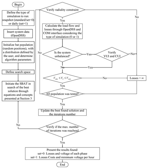
Figure 1.
SBAT to solve the DNR problem flowchart.
The summarized steps of the proposed approach are as follows:
- Step 1: Loading of all system data into EPRI-OpenDSS;
- Step 2: Definition and input of all SBAT parameters. The velocities and positions of the particles are uniformly distributed in a user-defined range. The search space (number of switches to be opened) is defined satisfying constraints of Section 2;
- Step 3: Start of the metaheuristic process. The search is performed using all equations of Section 3, where the values of frequency and the positions of the particles, i.e., bats, are updated using the best values as reference. The local search procedure is also conducted, and the pulse emission rate is checked. Initially, the values of bats’ positions are represented through continuous numbers. Posteriorly, these same values are approximated to selective values (representing the system switches) according to the sigmoid function and relation established in Section 3;
- Step 4: Switches are opened and the objective function is calculated through EPRI-OpenDSS. All constraints are checked. If the system is unbalanced, the additional checking of VUI and CUI is performed. If constraints are not attended, the solution is penalized;
- Step 5: Verification that all the population was tested. If not, the algorithm returns to Step 4; if yes, the algorithm jumps to Step 6;
- Step 6: Verification that the stoppage criteria, i.e., total number of iterations, were met. In a negative case, the present iteration number is incremented and the algorithm returns to Step 2. In a positive case, the algorithm stops and all proposed results are presented.
5. Results and Simulations
The tests were conducted mainly in two balanced systems (33- and 69-bus systems) and two unbalanced systems (19- and 25-bus system). These four cases were first carried out with a fixed power demand and then with a variable demand. The voltage limits constraint was established between 0.93 p.u. and 1.05 p.u. The voltage unbalance index (VUI) and current unbalance index (CUI) for unbalanced systems were established as 3% [41] and 30% [38], respectively, with a specific analysis for the influence of these indexes conducted. To assess the results found using the SBAT, a comparison with the traditional SPSO [46] and with a version of the selective harmony search (SHS) algorithm presented in [48] was carried out. Tests considered 100 runs for each system, with the exception of SHS for the 69-bus system with variable demand. In this case, only 25 tests were performed due to the high computational time required for each run. In addition, a brief analysis of DNR considering VUI and CUI on a modified 123-bus system was conducted and presented. All simulations were run on a notebook equipped with an Intel-Core i7 (California, US, Intel Corporation,) processor running on a Microsoft-Windows 10 (Washington, US, Microsoft Corporation) environment.
5.1. Algorithm Parameters
One of the crucial points for extracting better performance of bio-inspired metaheuristics is the setting of parameters. The SBAT presents a considerable amount of parameters to be adjusted, which may require some time to be defined properly. In addition to the proper algorithm parameters are those related to iterations and population, also needing a correct adjustment. Also, the variable demand cases must present the characteristics of all loads considered in the system, together with the hourly costs.
Regarding the SBAT, the parameters set were: , , , , and . The parameters and were empirically set through tests with values varying from zero to one, setting them to the best values found, i.e., 0.8. Regarding the values of , , and , these were set as those usually adjusted for most applications, as defined in [45] and cited in Section 3. The SPSO parameters, learning factor 1 , global learning factor 2 , maximum inertia weight , minimum inertia weight and maximum velocity V, were set as the default parameters of the PSO algorithm [49]. As for SHS parameters, harmony memory considering rate , pitch adjusting rate and bandwidth , they were set according to the values presented in [50]. The only exception is the number of improvisations , defined in the same way as the empirical test for the SBAT. These values were used in all simulations performed and are all described in Table 1.

Table 1.
Algorithms’ fixed parameters.
Population size, or harmony memory size (HMS) in the case of HS, and number of iterations for all algorithms were considered variable according to , described in Section 3. These values were defined to achieve a balance between convergence and computational time, aiming to extract a better performance from both points of view. Table 2 presents these values for the four main systems tested.
Table 2.
SBAT variable parameters.
As for the variable demand characteristics, the definitions found in [22,23] are followed and presented in Table 3. Residential, commercial and industrial loads were respectively identified as 1, 2 and 3. For each load type defined in Table 3, a cost (USD/kW) was associated with the respective hour together with a load factor. Each load located at a bus was characterized with a type described in Table 3. The selection for all systems, except the 33-bus system, was made through the Python function random.choice(), weighted with probabilities of 60%, 25% and 15% for choosing residential (Type 1), commercial (Type 2) or industrial (Type 3), respectively. The 33-bus system load distribution was taken from [51] for a comparative basis. For the unbalanced systems, the load types per phase in each bus were the same, e.g., bus 1 loads at phases A, B and C were residential. Finally, to compute the total losses costs when dealing with variable demand, simulations were performed considering 24 h for each configuration found, where the real losses costs in the current topology were determined at each specific hour of the day. The total losses costs in one day are represented through the sum of each of these costs in all hours. This procedure results in a final topology for one day, thus avoiding a constant state-changing of the system switches and preventing their wear out. With these definitions, it is possible to simulate DNR for the proposed systems.
Table 3.
Hourly costs and load profile (24 h).
5.2. Balanced Systems
Firstly, a 33-bus and 37-branch balanced system was considered, presenting a base voltage of 12.66 kV. All system data are found in [47].
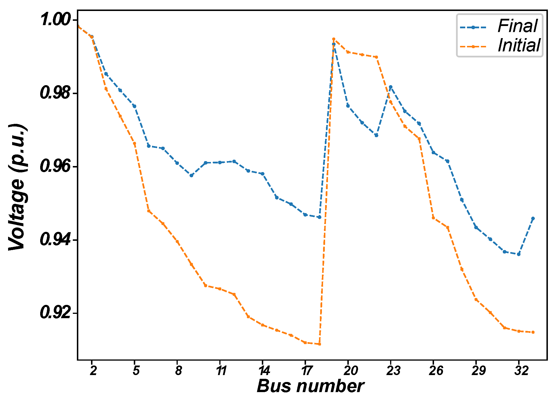
Initially considering a fixed demand and characteristics provided in Reference [47], the algorithm was tested in 100 runs and results are presented in Table 4. Figure 2 shows the voltage levels at each bus before and after the reconfiguration.
Table 4.
Results found for the 33-bus and 37-branch balanced system (fixed demand).
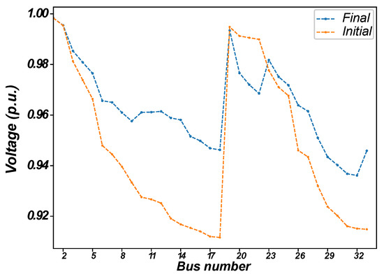
Figure 2.
33-bus and 37-branch system voltage levels (fixed).
Results in Table 4 show a 31.08% reduction in real losses, comparing initial and final distribution network configuration. From Figure 2, it is possible to assume that voltage levels were improved compared to the initial configuration, going from a minimum of 0.912 p.u. at bus 18 to 0.936 p.u. at bus 32. All results obtained are compatible with the technical literature [8,15,22,52].
In Table 4, a comparison between the SBAT, SPSO and SHS is also presented, showing which of the three found the best result. The SBAT overcame SPSO and SHS with a convergence rate of 96% and average losses of 139.74 kW.
The results provide a basis to consider the variable demand with the premises established in [22,23]. It is necessary to define the types of loads used in daily simulations. For the 33-bus case, this definition was (type of load/bus allocated): residential (2 to 4, 8 to 9, 11, 14 to 21, 23 to 25, 29, 31, 33), commercial (6 to 7, 10, 13, 22, 26 to 28, 30) and industrial (5, 12, 32).
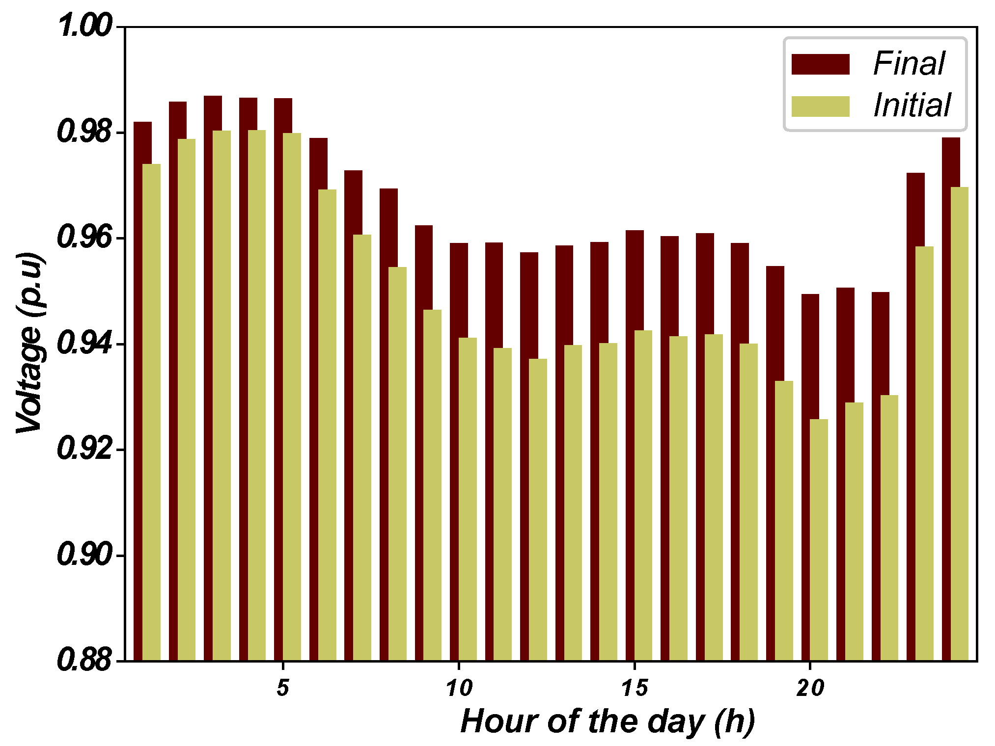
Table 5 describes results for variable demand. Figure 3 indicates minimum voltage levels for each hour along the day.
Table 5.
Results found for the 33-bus and 37-branch balanced system (variable demand).
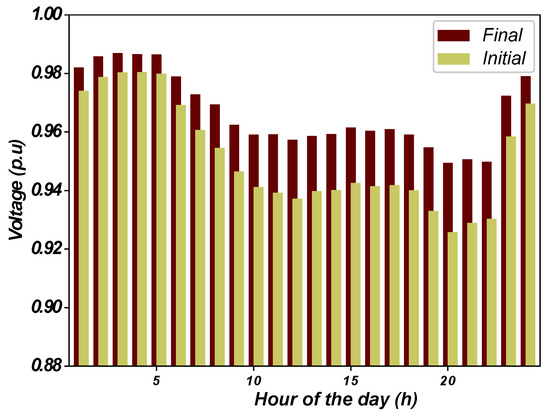
Figure 3.
33-bus and 37-branch system voltage levels (variable).
It is possible to verify from results in Table 5 that the new configuration reduced the total losses costs by 31.57% in comparison with the initial topology. In addition, it is possible to notice that the result is different from the one found considering fixed demand, pointing to opening switches 9-7-14-28-32 instead of 9-7-14-32-37, showing the importance of considering a variable load demand during simulations when searching for an optimum DNR. The minimum voltage levels also improved, going from initial 0.926 p.u. minimum at bus 18 (20 h) and 0.981 p.u. maximum-minimum at bus 18 (4 h) to final 0.951 p.u. minimum at bus 33 (20 h) and 0.987 p.u. maximum-minimum at bus 32 (3 h). All results are compatible with the results presented in [22,23] for the same system.
A comparison presented in Table 5 shows that the best solutions were also found by SPSO and SHS, but they had a worse performance in comparison with the SBAT. Selective PSO reached the best solution in 62% of all runs and an average total losses cost of 131.60 USD/kW. Selective HS reached the best solution in 72% of all runs and an average total losses cost of 130.02 USD/kW. Figure 4 and Figure 5 shows the final configuration and the open switches for fixed demand and variable demand respectively.
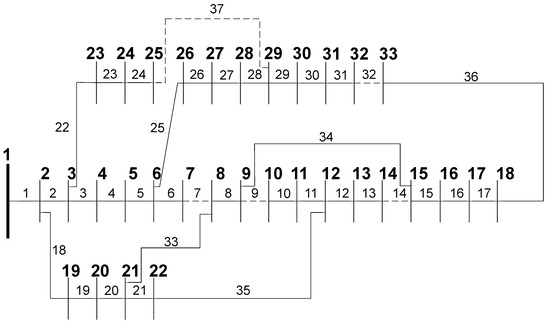
Figure 4.
33-bus and 37-branch system final configuration (fixed).

Figure 5.
33-bus and 37-branch system final configuration (variable).
The second balanced system presents 69 buses and 73 branches and is widely used in the literature. It was firstly presented in [53]. The base voltage of the system is 12.66 kV. Table 6 describes the results obtained for the SBAT. Figure 6 illustrates the respective initial and final voltage levels for each bus.
Table 6.
Results found for the 69-bus 73-branch balanced system (fixed demand).
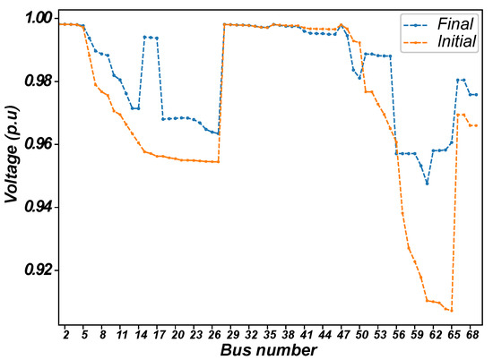
Figure 6.
69-bus and 73-branch system voltage levels (fixed).
All results found for this system (losses and voltage levels) in Table 6 and Figure 6 point to an improvement in the operative indexes after the reconfiguration. The losses reduced by 56.19% and the minimum voltage level increased from 0.907 p.u. at bus 69 to 0.948 p.u. at bus 65. Again, the results found are compatible with those in the specialized literature [54].
This case presents a particularity where different configurations, such as opening switches 55-61-70-69-14 or 56-61-70-69-14, show approximately the same percentage reduction and voltage levels as switches 58-61-70-69-14.
Table 6 also shows that the SBAT, SPSO and SHS reached the same solution, although the SBAT presented a better convergence to the best result (96%) and average final losses of 98.96 kW considering all runs. Selective PSO reached the best result in 31% of runs and an average final losses value of 108.07 kW. Selective HS reached the best result in only 8% of runs, although with a better average final losses value than SPSO (100.60 kW).
For the same system, now considering variable demand, the loads were defined as follows (load type/bus allocated): residential (9 to 10, 13 to 14, 16, 18, 20, 24, 26 to 29, 34, 39, 43, 45-46, 48, 50 to 51, 61 to 62, 64, 66 to 67, 69), commercial (7 to 8, 11, 17, 21, 33, 35, 37, 40, 49, 52, 55, 65, 68) and industrial (6, 12, 22, 41, 53 to 54, 59). As it is possible to notice, some buses are not connected to any type of load. Results obtained using the SBAT for the 69-bus balanced system with variable demand are presented in Table 7 and Figure 7.
Table 7.
Results found for the 69-bus and 73-branch balanced system (variable demand).
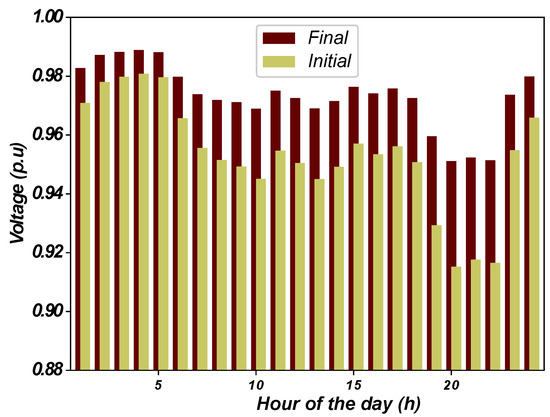
Figure 7.
69-bus and 73-branch system voltage levels (variable).
In the same way as the 33-bus test system, results show improvements in several indexes, such as total losses costs and minimum voltage profile. The first presented a decrease of 54.56% and the second an improvement, going from initial 0.915 p.u. minimum at bus 65 (20 h) and 0.981 p.u. maximum-minimum at bus 65 (4 h) to final 0.951 p.u. minimum at bus 61 (20 h) and 0.989 p.u. maximum-minimum at bus 61 (4 h). For this system, the set of switches defined as the best by the SBAT was the same as the one presented for the fixed demand case (58-61-70-69-14). There is no comparative basis in the technical literature in order to compare the obtained results to other results, taking into account the same premises in this research. The final configuration both for fixed and variable demand with its open switches is shown in Figure 8.
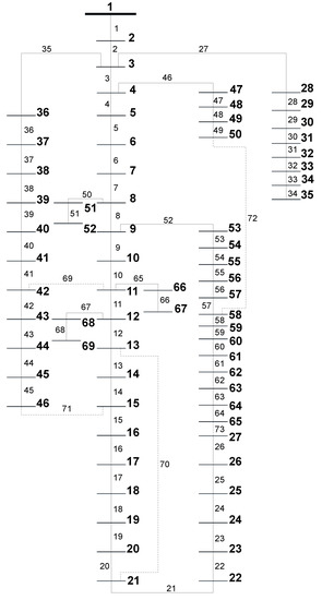
Figure 8.
69-bus and 73-branch system final configuration.
As presented for fixed demand, Table 7 shows also the results found by SPSO and SHS considering the same condition. Again, SPSO was able to find the best result, but with a convergence rate to this result of 27% and average total losses costs of 93.23 USD/kW, lower than the results found by the SBAT, which were respectively 95% and 85.41 USD/kW. Selective HS also found the best result, with a lower convergence rate to the best (8% for only 25 runs), but with a higher average total losses costs (86.34 USD/kW) than SPSO.
5.3. Unbalanced Systems
The study of unbalanced systems with variable demand considering unbalance indexes aims to better represent the characteristics of a real distribution system. The first unbalanced case studied was a 19-bus and 20-branch system with different load levels in each phase characterizing the imbalance [55]. The voltage base was 4.16 kV.
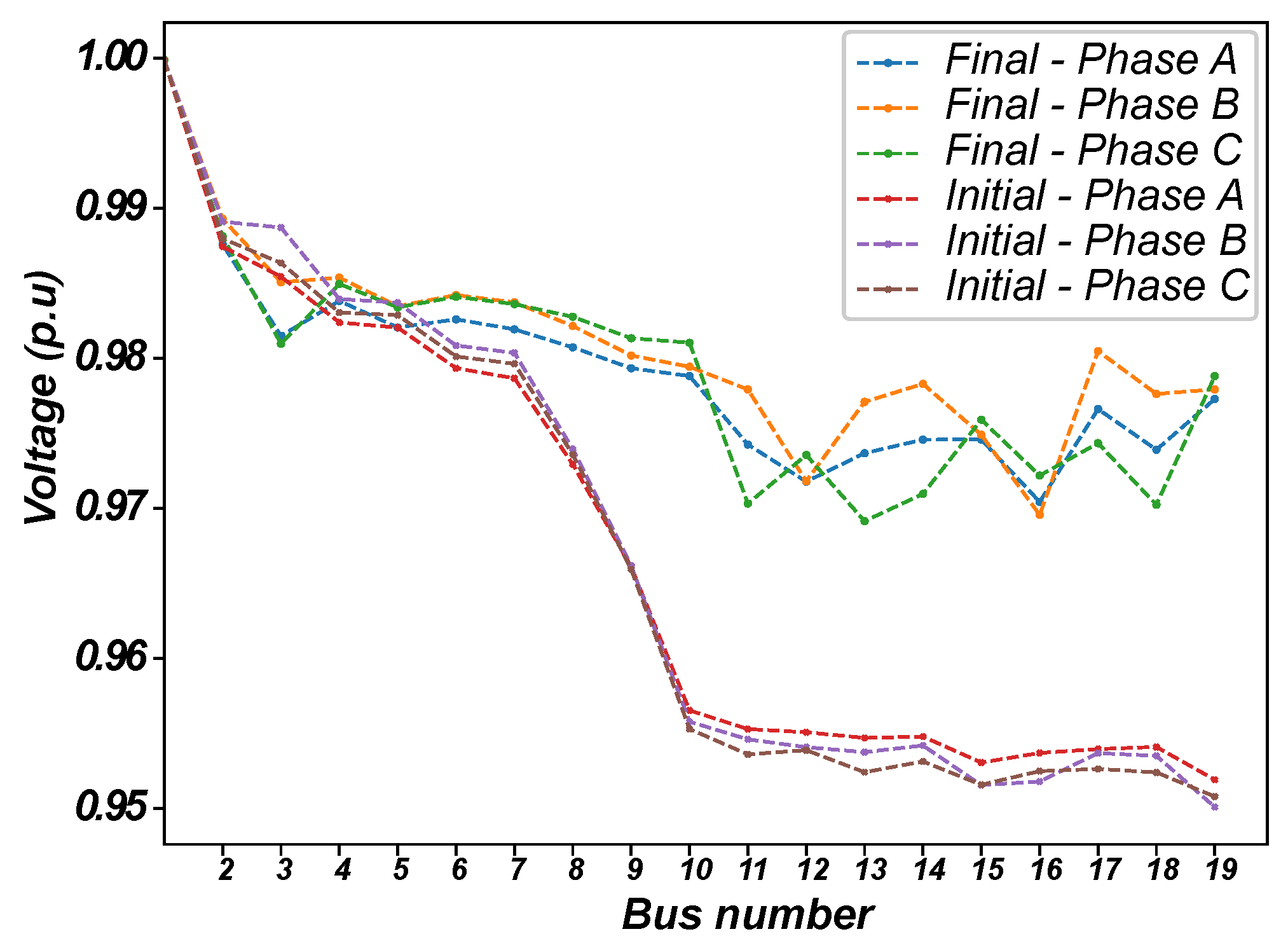
Initially, a fixed power demand was considered. Table 8 describes results for 100 runs, Table 9 shows the losses per phase before and after reconfiguration, and Figure 9 shows the voltage levels for each bus and each phase before and after reconfiguration.
Table 8.
Results found for the 19-bus and 20-branch unbalanced system (fixed demand).
Table 9.
Total losses per phase (19-bus system/fixed demand).
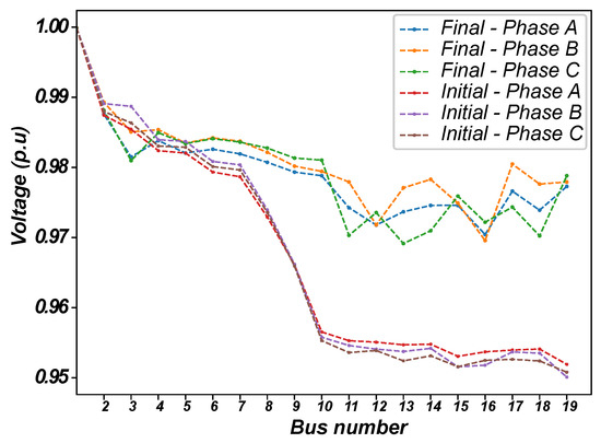
Figure 9.
19-bus and 20-branch system voltage levels (fixed).
The results found by the SBAT for this first test indicate opening switches 10-11, with an active losses reduction of 38.98% and a reduction in losses per phase. Voltage levels presented in Figure 9 show an improvement from initial to final configuration, from 0.950 p.u. minimum at bus 19 phase B and 0.999 p.u. maximum at bus 1 phase B to 0.969 p.u. minimum at bus 13 phase C and 0.999 p.u. maximum at bus 1 phase B. These results are compatible with those obtained in the literature [55]. For comparison, SPSO and SHS found the same results.
The solution found attends all limits established, i.e., voltage limits, VUI and CUI. The maximum values obtained for VUI and CUI through the solution were 0.42% and 25.31%, respectively.
If the CUI value of 25.31% is considered high, the minimum CUI limit that presents a feasible solution is 21%. Now, the new configuration with minimum losses that attends all constraints indicates opening switches 9-20, with a minimum and maximum voltage of 0.948 p.u. at bus 19 phase C and 0.999 p.u. at bus 1 phase B, maximum VUI of 0.24% and maximum CUI of 20.63%, reducing the total losses only by 8.85% with a final value of 12.05 kW.
For a variable power demand, the loads were considered as the same type for all phases in each bus and as the following (type of load/bus allocated): residential (2 to 4, 7 to 9, 10, 15 to 16), commercial (5 to 6, 12 to 13, 17) and industrial (1, 11, 14, 18).
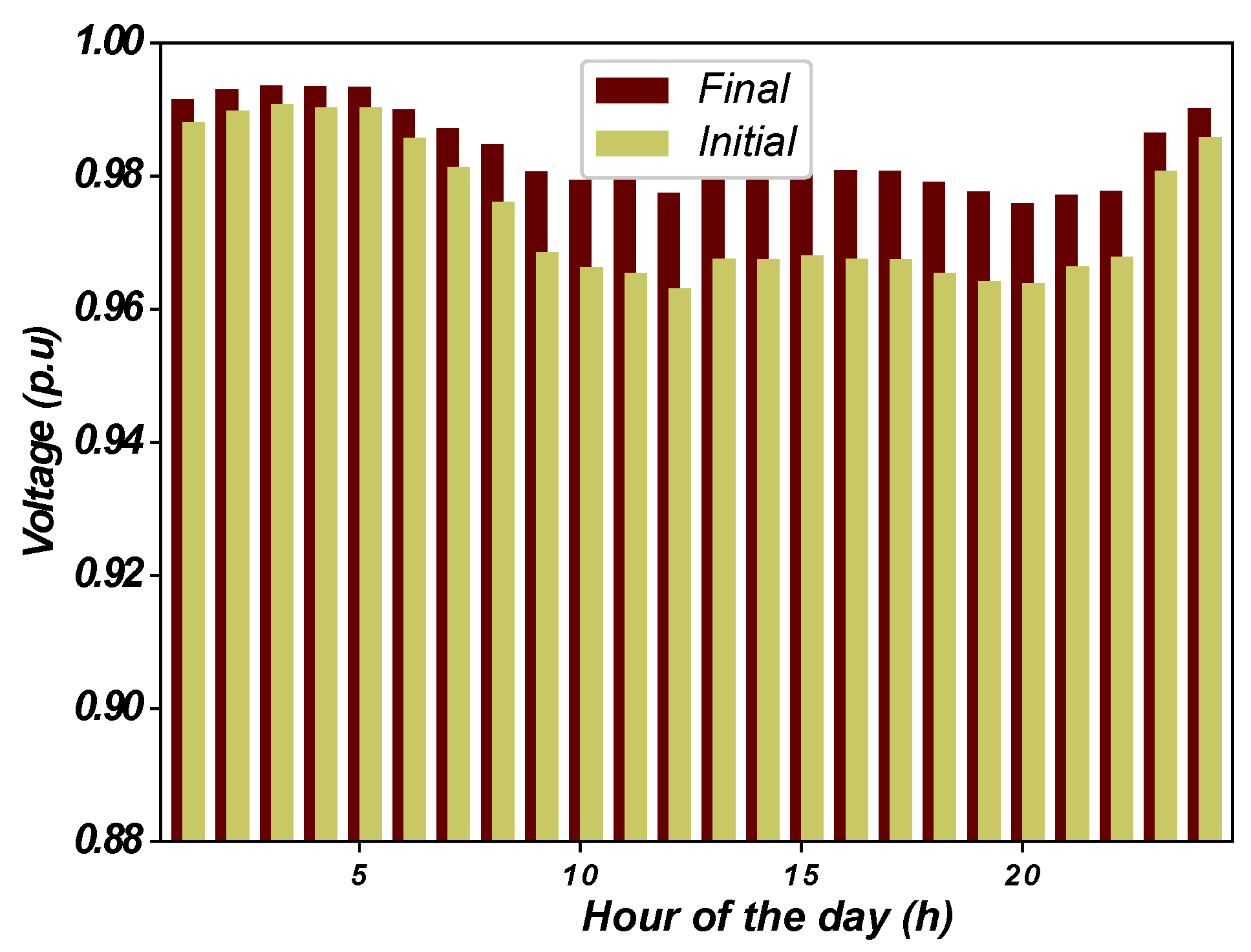
Results are presented in Table 10, with the total losses costs (USD), open switches, percentage costs reduction (%), average costs (USD) and convergence rate (%) for 100 runs. Table 11 shows the total losses costs per phase. Figure 10 illustrates the minimum voltage profile for 24 h.
Table 10.
Results found for the 19-bus and 20-branch balanced system (variable demand).
Table 11.
Total costs per phase in 24 h (19-bus system/variable demand).
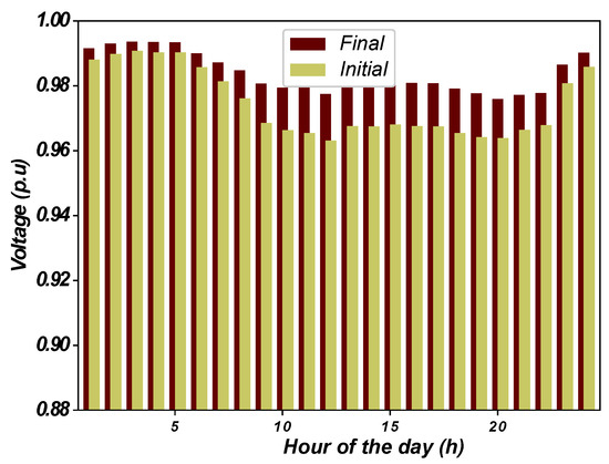
Figure 10.
19-bus and 20-branch system voltage levels (variable).
It is possible to infer from Table 10, Table 11 and Figure 10 that there was an improvement comparing the final with the initial configuration. The total costs reduced by 37.49%, indicating opening switches 13-11, and the total costs per phase reduced from 3.69 USD/kW, 3.69 USD/kW and 3.85 USD/kW in phases A, B and C, respectively, to 2.4 USD/kW, 2.14 USD/kW and 2.48 USD/kW. Similar to the 33-bus balanced case, simulations considering variable demand demonstrated different solutions in comparison with the fixed demand case, which indicated opening switches 10–11.
As for the minimum voltage levels, the 19-bus system’s minimum and minimum-maximum rose respectively from 0.963 p.u. at bus 19 phase C (12 h) and 0.991 p.u. at bus 13 phase C (3 h) p.u. to 0.976 p.u. and 0.994 p.u. The final minimum and minimum-maximum values were located at bus 16 phase B (19 h) and at bus 13 phase C (3 h). SPSO and SHS found the same results, as shown in Table 10.
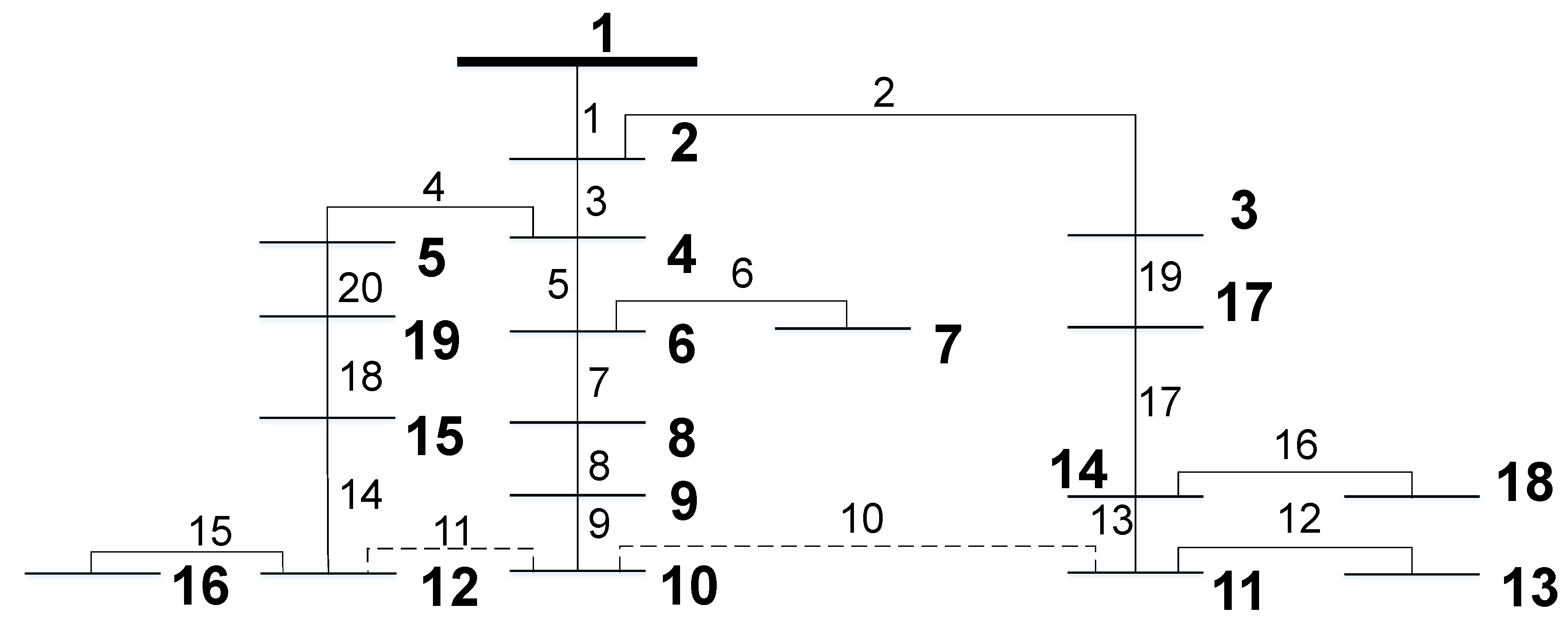
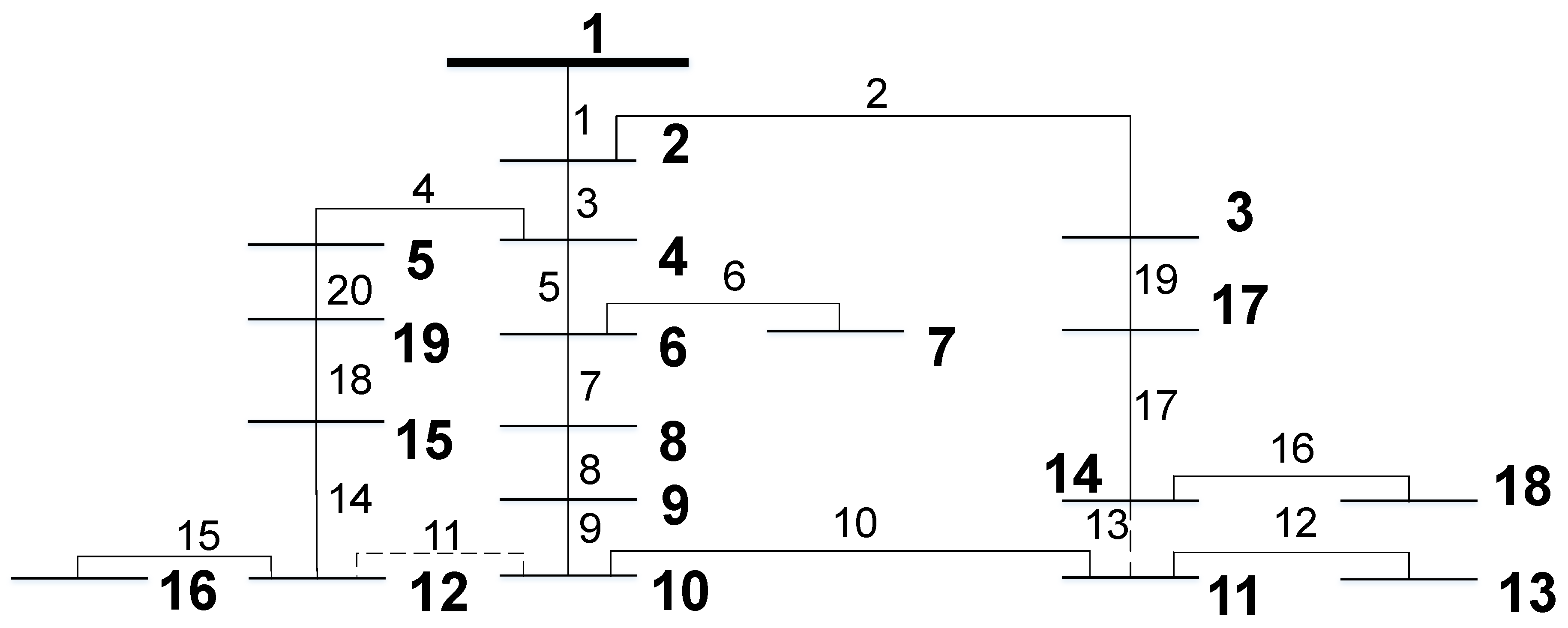
The maximum VUI and CUI values obtained when opening switches 13 and 11 were respectively 0.21% and 26.02%, attending the established limits. Again, the value of VUI is low, but CUI may be considered high. The minimum value of CUI to obtain a feasible solution for this system with variable demand is 22%, which indicates opening switches 9–20, obtaining a maximum absolute VUI of 0.21%, a maximum absolute CUI of 21.18%, a minimum voltage of 0.960 p.u. at bus 19 phase C (12 h) and a maximum-minimum voltage of 0.991 p.u. at bus 16 phase C (3 h), with total losses costs of 10.22 USD/kW for a 24 h period. Figure 11 and Figure 12 shows respectively the final configuration for the fixed and variable demand.
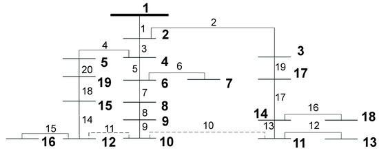
Figure 11.
19-bus and 20-branch system final configuration (fixed).
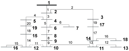
Figure 12.
19-bus and 20-branch system final configuration (variable).
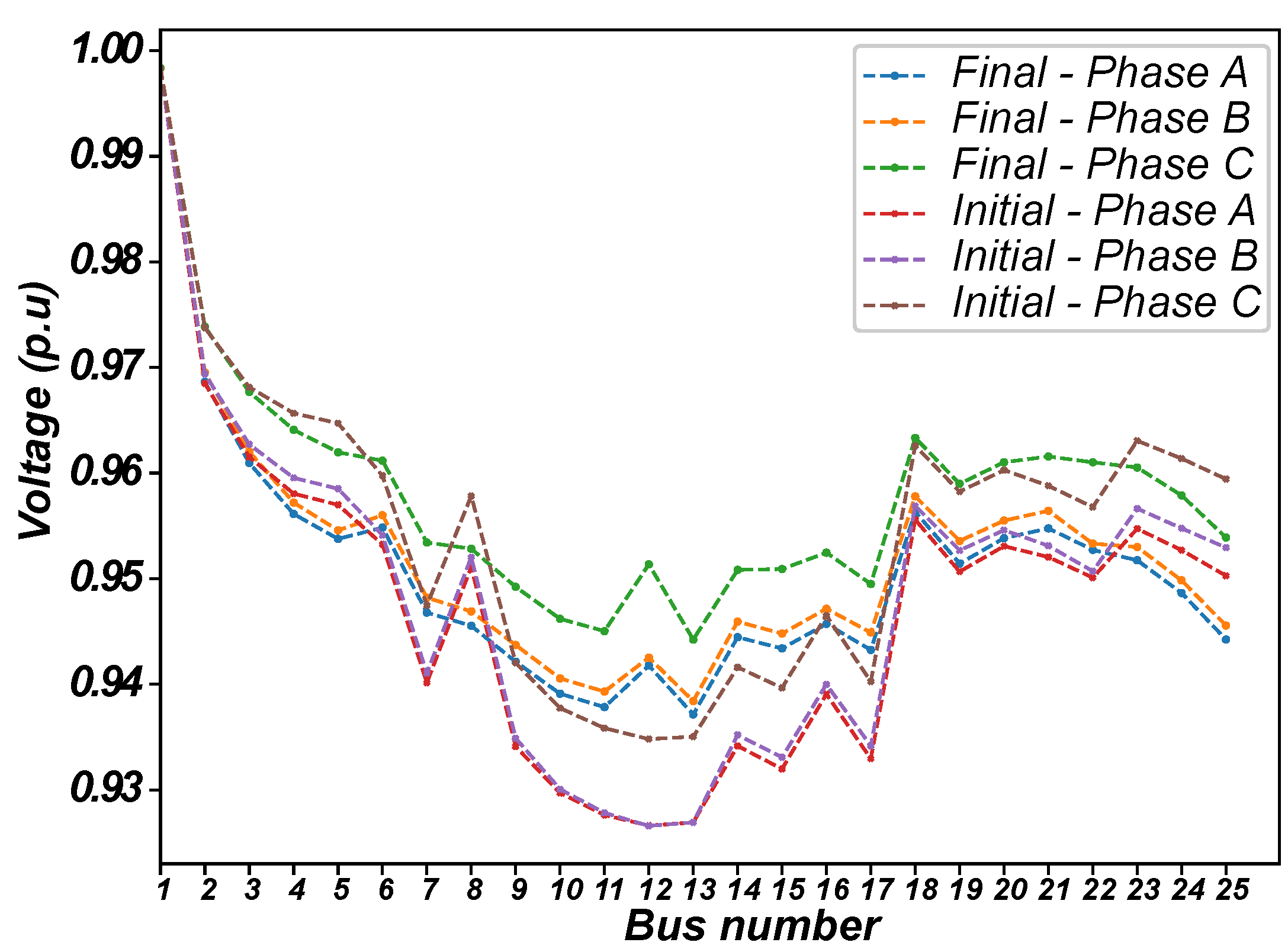
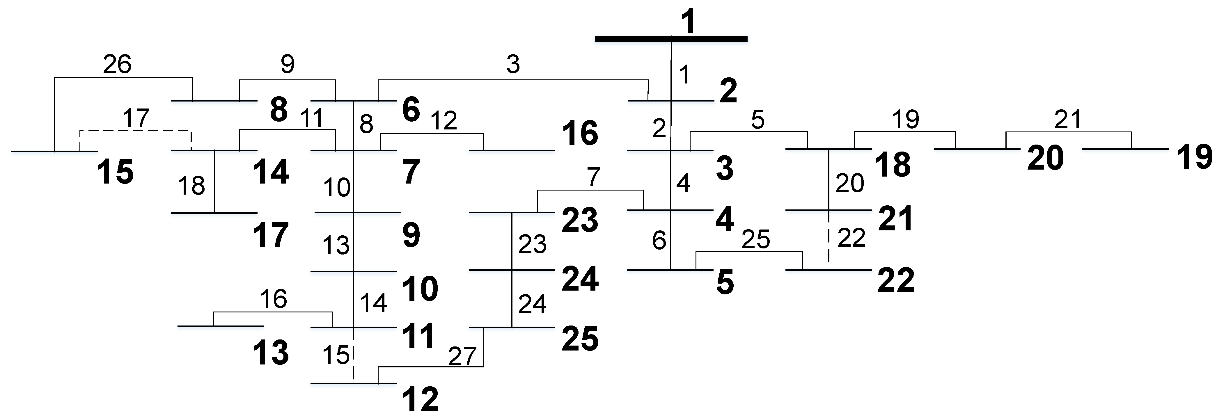
The second unbalanced system tested is composed of 25 buses and 27 branches, as presented in [55,56,57], with a base voltage of 4.16 kV and imbalance between phase loading. Results are presented in Table 12, Table 13 and Figure 13.
Table 12.
Results found for the 25-bus and 27-branch unbalanced system (fixed demand).
Table 13.
Total losses per phase (25-bus system/fixed demand).

Figure 13.
25-bus and 27-branch system voltage levels (fixed).
Results for all algorithms (SBAT, SPSO and SHS) show the decrease in loss levels (10.79%) when comparing the initial open switches, 25-26-27, with those determined after the DNR, 22-15-17, as well as a decrease in losses per phase. In addition, there was an improvement in the general voltage levels, with the minimum value increasing from 0.927 p.u. at bus 12 phase B to 0.937 p.u. at bus 13 phase A. The maximum voltage level was 0.998 p.u. at bus 1 phase A in the initial and final configurations. The results are compatible with those found in [55,56,57].
The maximum VUI and CUI values for the solution 22-15-17 are respectively 0.65% and 12.84%, attending the established limits of 3% and 30%. In the same way as the 19-bus system, if the CUI is considered high, a new limit must be set. The minimum limit value that presents a feasible solution is 12.83%, indicating opening switches 22-26-15, reducing losses to 141.85 kW and presenting minimum voltage of 0.937 p.u. at bus 13 phase A, maximum voltage of 0.998 p.u. at bus 1 phase A and maximum VUI and CUI of 0.65% and 12.828%, respectively. The VUI and CUI values were slightly lower than the original solution.
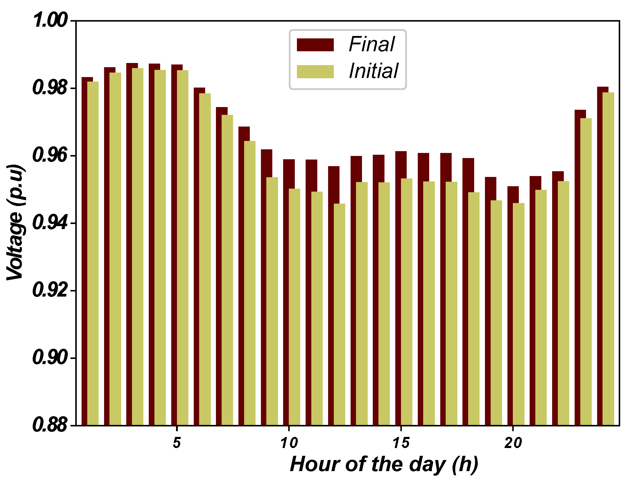
For the variable demand case, the loads were defined as the same type for all phases in each bus as follows (type of load/bus allocated): residential (1, 5, 7, 9 to 11, 16 to 18, 21, 23, 25), commercial (15, 20, 22, 24) and industrial (3 to 4, 6, 8, 12 to 13, 19). Table 14 and Table 15 and Figure 14 present the results, total losses costs per phase and minimum voltage levels for 24 h, respectively.
Table 14.
Results found for the 25-bus and 27-branch balanced system (variable demand).
Table 15.
Total costs per phase in 24 h (25-bus system/variable demand).

Figure 14.
25-bus and 27-branch system voltage levels (variable).
Table 14 shows that the results for the three algorithms (SBAT, SPSO and SHS) indicate the same set of opened switches in the fixed demand case (25-15-17). The total losses costs diminished from 131.58 USD to 117.51 USD, representing a reduction of 10.71%. Table 15 shows an improvement in the total losses costs per phase for a 24 h period. The minimum voltage levels in Figure 14 also improved, from 0.947 p.u. minimum at bus 12 phase B (12 h) and 0.986 p.u. minimum-maximum at bus 15 phase A (3 h) to 0.951 p.u. minimum and 0.987 p.u. minimum-maximum. The final minimum and minimum-maximum values were located at bus 13 phase A (20 h) and at bus 13 phase A (3 h). Figure 15 brings the final configuration for the 25-bus system considering both fixed and variable demand.
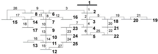
Figure 15.
25-bus and 27-branch system.
The maximum VUI and CUI presented for the solution 25-15-17 with variable demand were 0.46% and 13.41%, attending the limits established. For CUI, if the limit is considered high, the minimum limit value that presents a feasible solution reducing losses is 13%, which indicates opening switches 22-17-14, with a maximum VUI and CUI of 0.49% and 12.95%, respectively, minimum voltage of 0.945 p.u. at bus 13 phase B (12 h) and maximum-minimum voltage of 0.986 p.u. at bus 13 phase A (3 h), reducing losses costs to 119.39 USD/kW.
5.4. Additional Test
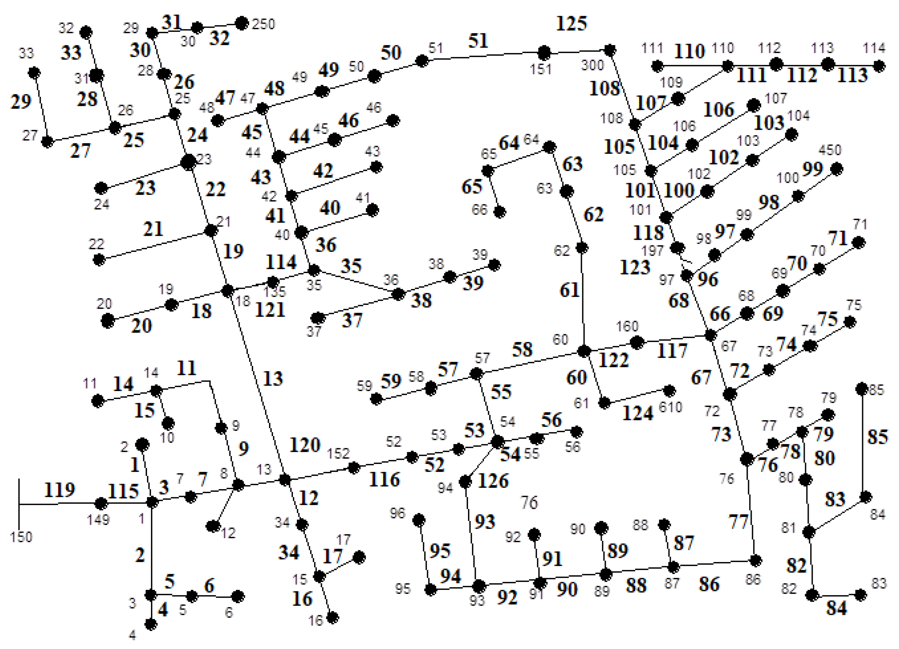
Additionally, a modified 123-bus system, presented in Figure 16, was tested. This system was originally composed of voltage regulators, capacitor banks, single and three-phase sections, different types of cables and underground sections, among other characteristics described in [58]. To assess the system only from the reconfiguration point of view, the system was modified, excluding all equipment.
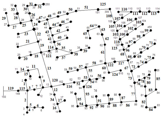
Figure 16.
123-bus modified system.
However, when considering both VUI and CUI limits, this system did not present a feasible solution, as, although VUI presented values under 3%, CUI surpassed the value of 30% by a larger margin, as some sections of the system presented currents of low value (almost zero). For example, consider branch 22 of the modified system, which presented currents of magnitude 54.775 A in phase A, 0.004 A in phase B and 58.477 A in phase C. This happens also in this same branch of the system in its original state (considering all equipment) [58], with currents of magnitude 55.853 A in phase A, 0.005 A in phase B, and 55.404 A in phase C, which points out a highly unbalanced characteristic from the point of view of currents.
A solution for both fixed and variable demand is only found when disregarding CUI constraint in the same way as the majority of papers dealing with DNR and unbalanced systems present. In addition, the minimum voltage level allowed, which is established as 0.93 p.u. in this paper for all systems, must be set to 0.9 p.u. for this system in fixed demand to find a minimum losses solution.
For fixed demand, the algorithm indicates opening switches 118-93 with losses of 105.68 kW, as opposed to the initial open switches 125-126 with losses of 109.12 kW. The voltage levels also improved, going from 0.912 p.u. minimum at bus 114 phase A to 0.918 p.u minimum at bus 114 phase A and maintaining 0.999 p.u as maximum at bus 150 phase B.
As for variable demand, the loads were divided as follows: residential (1, 2, 5, 6 to 9, 12, 19, 20, 28 to 30, 32 to 35, 37, 38, 42, 43, 45 to 50, 53, 55, 58, 59, 62, 65, 66, 73, 76, 83, 85 to 88, 90, 92, 94, 96, 100, 103, 104, 106, 107, 109, 111 to 113), commercial (4, 7, 17, 24, 52, 60, 63, 64, 70, 74, 79, 95, 98, 99) and industrial (16, 22, 31, 39, 41, 51, 56, 68, 69, 71, 75, 80, 82, 84, 102, 114). The algorithm indicates opening switches 125-93 with total losses costs of 95.6 USD as opposed to the initial set of open switches 125-126 with costs of 96.5 USD. The voltage levels, minimum and minimum–maximum, also improved, going from 0.928 p.u. to 0.931 p.u. at bus 114 phase A (20 h) and from 0.980 p.u. to 0.981 p.u. at bus 150 phase B (3 h).
This example helps to emphasize the influence of the unbalance indexes, especially CUI, when finding a solution for the DNR problem in unbalanced systems, as these constraints, when considered, can directly determine a feasible or unfeasible solution to the problem.
5.5. VUI and CUI Influence Analysis
The influence of VUI and CUI can be summarized in Table 16 for the two main unbalanced systems studied (considering fixed and variable demand).
Table 16.
VUI and CUI for unbalanced systems.
The results consolidated in Table 16 show the direct influence of VUI and CUI in DNR results for these two systems. When considering the limits established for all systems, i.e., 3% for VUI and 30% for CUI, the results are the same as those found when disregarding these two constraints.
However, when slightly decreasing the CUI limits allowed in all systems to the minimum values that present a feasible solution, new topologies were found in comparison with those for the limit of 30%, hence reducing the current unbalance. These different solutions were seen for both demand cases in some systems, for example, the 25-bus unbalanced system, which presented three different solutions depending on the value of CUI considered and the demand level studied. In some cases, the value of VUI also decreased alongside the new value of CUI established, as in the case of 19-bus unbalanced system with fixed demand. In addition, the feasible solution with the minimum CUI increased the values of losses and losses costs in the majority of cases.
The presented analysis indicated that the DNR in unbalanced systems is indeed sensible to these indexes, particularly CUI, as it is the index that presented higher values in all systems, greater affecting the results found. This is clearly seen for the additional 123-bus system presented, as it is difficult to find a feasible solution when CUI is considered in the problem. Although all systems analysis, including that of the 123-bus system, could be easily carried out only in the VUI context or without these two constraints, as results show, the assessment of CUI may be important in some cases, as high values of CUI can cause the earlier stated difficulties related to protection [37] and to power and energy losses [38], emphasizing the importance of the assessment of this index in DNR problems.
5.6. Convergence Analysis
To justify the choice of the SBAT in favor of other techniques, a convergence analysis for four of the studied systems (with the exception of the additional 123-bus system) considering both fixed and variable demand is presented. Table 17 and Table 18 show the minimum iterations to the best result, the maximum iterations to the best result, the minimum time to the best result, the maximum time to the best result and the average time to the best result for all methods.
Table 17.
Convergence analysis SBAT/SPSO/SHS—fixed demand.
Table 18.
Convergence analysis SBAT/SPSO—variable demand.
The convergence analysis presented in Table 17 and Table 18 shows, in general, a better performance for the SBAT in comparison with SPSO and SHS, as previously presented by the convergence to the best result and confirmed by the average times to find the best results for the SBAT. The minimum iterations to the best result also show a slight advantage for the SBAT. As for the maximum iterations to the best and the computational time, in the majority of cases, the performances for the SBAT and SPSO were close. SHS presented a higher computational time when establishing the same premises used for both the SBAT and SPSO, presenting a low convergence rate in systems with higher numbers of switches (e.g., 69-bus) with variable demand, thus limiting the number of runs used for comparison (e.g., 25 runs). In general, in this paper, the SBAT appears as the better alternative to solve the DNR problem.
6. Conclusions
Here, a proposal to solve the DNR problem through a bio-inspired metaheuristic (SBAT) for unbalanced systems with variable demand considering VUI and CUI was presented. As the DNR problem is conventionally approached by single-phase balanced modeling with fixed power demand, the approach presented is closer to the real characteristics of distribution systems. In addition, the analysis of the influence of VUI and CUI in the results for all unbalanced systems represents the novel contribution of the proposed manuscript.
The simulations performed for balanced and unbalanced networks with fixed or variable demand find values compatible with the literature, maintaining the voltage and power stability in all cases, and, for unbalanced cases, attending, in the majority of cases, the established limits of VUI and CUI, thus confirming the adequacy of the results and the model here proposed. It is shown that VUI and CUI can influence the selection of switches to be opened depending on the admissible limits set for the network, directly affecting the DNR process.
All results presented for the unbalanced cases considering the demand as variable, together with VUI and CUI, encourage us to apply this model in future studies on larger and real systems. Studies presenting an in-depth analysis of systems in the presence of other power devices (e.g., regulators, capacitor banks or transformers) and how they influence the values of these indexes together with DNR and of systems with different constructive characteristics (e.g., composed of underground cables) may also be carried out. Another analysis that is proposed to future studies is to solve the problem through mathematical and numerical methods (e.g., convex relaxation).
In addition, further studies that consider smart-grids, e.g., electric vehicles, together with distributed generation are also a possibility, as the penetration of such is constantly increasing and the nature of distribution networks is changing, together with the development of these new concepts. In this way, a more complete and even closer-to-reality model of a distribution network can be assessed.
Author Contributions
Conceptualization, C.G., E.C.M.C. and A.J.S.F.; investigation, C.G., E.C.M.C. and A.J.S.F.; writing—original draft preparation, C.G.; writing—review and editing, C.G., E.C.M.C. and A.J.S.F.; supervision, E.C.M.C. and A.J.S.F.; funding acquisition, C.G. and E.C.M.C. All authors have read and agreed to the published version of the manuscript.
Funding
CNPq—National Council of Scientific and Technological Research (grant no. 142049/2018-2).
Institutional Review Board Statement
Not applicable.
Informed Consent Statement
Not applicable.
Data Availability Statement
No new data were created or analyzed in this study.
Acknowledgments
The authors would like to thank CNPq, the National Council of Scientific and Technological Research, for the financial support.
Conflicts of Interest
The authors declare that they have no conflict of interest or competing interest.
References
- Gerez, C.; Silva, L.I.; Belati, E.A.; Filho, A.J.S.; Costa, E.C.M. Distribution Network Reconfiguration Using Selective Firefly Algorithm and a Load Flow Analysis Criterion for Reducing the Search Space. IEEE Access 2019, 7, 67874–67888. [Google Scholar] [CrossRef]
- Nguyen, T.T.; Nguyen, T.T.; Nguyen, N.A.; Duong, T.L. A novel method based on coyote algorithm for simultaneous network reconfiguration and distribution generation placement. Ain Shams Eng. J. 2020, 12, 665–676. [Google Scholar] [CrossRef]
- Merlin, A.; Back, H. Search for a Minimal-Loss Operating Spanning Tree Configuration in an Urban Power Distribution System. In Proceedings of the 5th Power System Computation Conference (PSCC), Cambridge, UK, 1–5 September 1975; pp. 1–18. [Google Scholar]
- Chang, H.C.; Kuo, C.C. Network reconfiguration in distribution systems using simulated annealing. Electr. Power Syst. Res. 1994, 29, 227–238. [Google Scholar] [CrossRef]
- Kim, H.; Ko, Y.; Jung, K.H. Artificial neural-network based feeder reconfiguration for loss reduction in distribution systems. IEEE Trans. Power Deliv. 1993, 8, 1356–1366. [Google Scholar] [CrossRef]
- Nara, K.; Shiose, A.; Kitagawa, M.; Ishihara, T. Implementation of Genetic Algorithm for Distribution Systems Loss Minimum Re-Configuration. IEEE Trans. Power Syst. 1992, 7, 1044–1051. [Google Scholar] [CrossRef]
- Su, C.-T.; Chang, C.-F.; Chiou, J.-P. Distribution network reconfiguration for loss reduction by ant colony search algorithm. Electr. Power Syst. Res. 2005, 75, 190–199. [Google Scholar] [CrossRef]
- Martín, J.A.; Gil, A.J. A new heuristic approach for distribution systems loss reduction. Electr. Power Syst. Res. 2008, 78, 1953–1958. [Google Scholar] [CrossRef]
- Abdelaziz, A.Y.; Mohammed, F.M.; Mekhamer, S.F.; Badr, M.A.L. Distribution Systems Reconfiguration using a modified particle swarm optimization algorithm. Electr. Power Syst. Res. 2009, 79, 1521–1530. [Google Scholar] [CrossRef]
- Abdelaziz, A.Y.; Mohamed, F.M.; Mekhamer, S.F.; Badr, M.A.L. Distribution system reconfiguration using a modified Tabu Search algorithm. Electr. Power Syst. Res. 2010, 80, 943–953. [Google Scholar] [CrossRef]
- Abdelaziz, A.Y.; Osama, R.A.; Elkhodary, S.M. Distribution Systems Reconfiguration Using Ant Colony Optimization and Harmony Search Algorithms. Electr. Power Components Syst. 2013, 41, 537–554. [Google Scholar] [CrossRef]
- Naveen, S.; Sathish Kumar, K.; Rajalakshmi, K. Distribution system reconfiguration for loss minimization using modified bacterial foraging optimization algorithm. Int. J. Electr. Power Energy Syst. 2015, 69, 90–97. [Google Scholar] [CrossRef]
- Nguyen, T.T.; Truong, A.V. Distribution network reconfiguration for power loss minimization and voltage profile improvement using cuckoo search algorithm. Int. J. Electr. Power Energy Syst. 2015, 68, 233–242. [Google Scholar] [CrossRef]
- Nguyen, T.T.; Truong, A.V.; Phung, T.A. A novel method based on adaptive cuckoo search for optimal network reconfiguration and distributed generation allocation in distribution network. Int. J. Electr. Power Energy Syst. 2016, 78, 801–815. [Google Scholar] [CrossRef]
- Nguyen, T.T.; Nguyen, T.T.; Truong, A.V.; Nguyen, Q.T.; Phung, T.A. Multi-objective electric distribution network reconfiguration solution using runner-root algorithm. Appl. Soft Comput. J. 2017, 52, 93–108. [Google Scholar] [CrossRef]
- Pegado, R.; Ñaupari, Z.; Molina, Y.; Castillo, C. Radial distribution network reconfiguration for power losses reduction based on improved selective BPSO. Electr. Power Syst. Res. 2019, 169, 206–213. [Google Scholar] [CrossRef]
- Landeros, A.; Koziel, S.; Abdel-Fattah, M.F. Distribution network reconfiguration using feasibility-preserving evolutionary optimization. J. Mod. Power Syst. Clean Energy 2019, 7, 589–598. [Google Scholar] [CrossRef] [Green Version]
- Rahimi Pour Behbahani, M.; Jalilian, A.; Amini, M.A. Reconfiguration of distribution network using discrete particle swarm optimization to reduce voltage fluctuations. Int. Trans. Electr. Energy Syst. 2020, 30, e12501. [Google Scholar] [CrossRef]
- Kazemi-Robati, E.; Sepasian, M.S. Fast heuristic methods for harmonic minimization using distribution system reconfiguration. Electr. Power Syst. Res. 2020, 181, 106185. [Google Scholar] [CrossRef]
- Raut, U.; Mishra, S. An improved sine–Cosine algorithm for simultaneous network reconfiguration and DG allocation in power distribution systems. Appl. Soft Comput. J. 2020, 92, 106293. [Google Scholar] [CrossRef]
- Kahouli, O.; Alsaif, H.; Bouteraa, Y.; Ben Ali, N.; Chaabene, M. Power system reconfiguration in distribution network for improving reliability using genetic algorithm and particle swarm optimization. Appl. Sci. 2021, 11, 3092. [Google Scholar] [CrossRef]
- Souza, S.S.; Romero, R.; Pereira, J.; Saraiva, J.T. Artificial Immune Algorithm Applied to Distribution System Reconfiguration with Variable Demand. Int. J. Electr. Power Energy Syst. 2016, 82, 561–568. [Google Scholar] [CrossRef] [Green Version]
- Possagnolo, L.H.F.M. Reconfiguração de sistemas de distribuição operando em vários níveis de demanda através de uma meta-heurística de busca em vizinhança variável. Master’s Thesis, Universidade Estadual Paulista Júlio de Mesquita Filho—UNESP, Ilha Solteira, Brasil, 2015. [Google Scholar]
- Hesaroor, K.; Das, D. Annual energy loss reduction of distribution network through reconfiguration and renewable energy sources. Int. Trans. Electr. Energy Syst. 2019, 29, e12099. [Google Scholar] [CrossRef]
- Nguyen, T.T.; Nguyen, T.T.; Duong, L.T.; Truong, V.A. An effective method to solve the problem of electric distribution network reconfiguration considering distributed generations for energy loss reduction. Neural Comput. Appl. 2021, 33, 1625–1641. [Google Scholar] [CrossRef]
- Zimmerman, R.D. Network Reconfiguration for Loss Reduction in Three-Phase Power Distribution Systems. Master’s Thesis, Cornell University, Ithaca, NY, USA, 1992. [Google Scholar]
- Darling, G. An efficient algorithm for real-time network reconfiguration in large scale unbalanced distribution systems. IEEE Trans. Power Syst. 1996, 11, 511–517. [Google Scholar] [CrossRef]
- Borozan, V. Minimum loss reconfiguration of unbalanced distribution networks. IEEE Power Eng. Rev. 1997, 17, 64. [Google Scholar] [CrossRef]
- Gangwar, P.; Singh, S.N.; Chakrabarti, S. Multi-objective planning model for multiphase distribution system under uncertainty considering reconfiguration. IET Renew. Power Gener. 2019, 13, 2070–2083. [Google Scholar] [CrossRef]
- Zheng, W.; Huang, W.; Hill, D.J. A deep learning-based general robust method for network reconfiguration in three-phase unbalanced active distribution networks. Int. J. Electr. Power Energy Syst. 2020, 120, 105982. [Google Scholar] [CrossRef]
- Zidan, A.; Farag, H.E.; El-Saadany, E.F. Network reconfiguration in balanced and unbalanced distribution systems with high DG penetration. In Proceedings of the 2012 IEEE Power and Energy Society General Meeting, San Diego, CA, USA, 22–26 July 2012; pp. 1–8. [Google Scholar] [CrossRef]
- Zidan, A.; El-Saadany, E.F. Network reconfiguration in balanced and unbalanced distribution systems with variable load demand for loss reduction and service restoration. In Proceedings of the IEEE Power and Energy Society General Meeting, San Diego, CA, USA, 22–26 July 2012. [Google Scholar] [CrossRef]
- Ding, F.; Loparo, K.A. Feeder Reconfiguration for Unbalanced Distribution Systems with Distributed Generation: A Hierarchical Decentralized Approach. IEEE Trans. Power Syst. 2016, 31, 1633–1642. [Google Scholar] [CrossRef]
- Gangwar, P.; Mallick, A.; Chakrabarti, S.; Singh, S.N. Short-Term Forecasting-Based Network Reconfiguration for Unbalanced Distribution Systems with Distributed Generators. IEEE Trans. Ind. Inform. 2020, 16, 4378–4389. [Google Scholar] [CrossRef]
- Mohamed, M.A.; Ali, Z.M.; Ahmed, M.; Al-Gahtani, S.F. Energy Saving Maximization of Balanced and Unbalanced Distribution Power Systems via Network Reconfiguration and Optimum Capacitor Allocation Using a Hybrid Metaheuristic Algorithm. Energies 2021, 14, 3205. [Google Scholar] [CrossRef]
- Zhai, H.F.; Yang, M.; Chen, B.; Kang, N. Dynamic reconfiguration of three-phase unbalanced distribution networks. Int. J. Electr. Power Energy Syst. 2018, 99, 1–10. [Google Scholar] [CrossRef]
- Peppanen, J.; Damato, G.; Araiza, J.; Kedis, M.; Sanchez, I. Analysis of Current and Voltage Unbalance from Distribution Systems with High der Penetration. In Proceedings of the IEEE Power and Energy Society General Meeting, Atlanta, GA, USA, 4–8 August 2019. [Google Scholar] [CrossRef]
- Arghavani, H.; Peyravi, M. Unbalanced current-based tariff. CIRED—Open Access Proc. J. 2017, 2017, 883–887. [Google Scholar] [CrossRef]
- Yang, X.S.; Cui, Z.; Xiao, R.; Gandomi, A.H.; Karamanoglu, M. Swarm Intelligence and Bio-Inspired Computation: Theory and Applications, 1st ed.; Elsevier Science Publishers B. V.: Amsterdam, The Netherlands, 2013. [Google Scholar]
- Monteiro, R.V.A.; Bonaldo, J.P.; da Silva, R.F.; Bretas, A.S. Electric distribution network reconfiguration optimized for PV distributed generation and energy storage. Electr. Power Syst. Res. 2020, 184, 106319. [Google Scholar] [CrossRef]
- Mostafa, H.A.; El-Shatshat, R.; Salama, M.M. Phase balancing of a 3-phase distribution system with a considerable penetration of single phase solar generators. In Proceedings of the IEEE Power Engineering Society Transmission and Distribution Conference, Chicago, IL, USA, 14–17 April 2014. [Google Scholar] [CrossRef]
- Dugan, R.C. Reference Guide: The Open Distribution System Simulator (OpenDSS); Electric Power Research Institute, Inc.: Palo Alto, CA, USA, 2013; pp. 1–177. [Google Scholar]
- Yang, X.S. A New Metaheuristic Bat-Inspired Algorithm BT—Nature Inspired Cooperative Strategies for Optimization (NICSO 2010); Springer: Berlin/Heidelberg, Germany, 2010; pp. 65–74. [Google Scholar]
- Yang, X.S. Nature-Inspired Optimization Algorithms, 1st ed.; Elsevier: Oxford, UK, 2014; p. 258. [Google Scholar] [CrossRef]
- Yang, X.S. Bat algorithm for multi-objective optimisation. Int. J. -Bio-Inspired Comput. 2011, 3, 267–274. [Google Scholar] [CrossRef]
- Khalil, T.M.; Gorpinich, A.V. Selective Particle Swarm Optimization. Int. J. Multidiscip. Sci. Eng. 2012, 3, 2–5. [Google Scholar]
- Baran, M.; Wu, F. Network reconfiguration in distribution systems for loss reduction and load balancing. IEEE Trans. Power Deliv. 1989, 4, 1401–1407. [Google Scholar] [CrossRef]
- Geem, Z.W. Harmony Search in Water Pump Switching Problem BT—Advances in Natural Computation; Springer: Berlin/Heidelberg, Germany, 2005; pp. 751–760. [Google Scholar]
- Juneja, M.; Nagar, S.K. Particle swarm optimization algorithm and its parameters: A review. In Proceedings of the 2016 International Conference on Control, Computing, Communication and Materials (ICCCCM), Allahabad, India, 21–22 October 2016; pp. 1–5. [Google Scholar] [CrossRef]
- Rao, R.S.; Ravindra, K.; Satish, K.; Narasimham, S.V. Power loss minimization in distribution system using network reconfiguration in the presence of distributed generation. IEEE Trans. Power Syst. 2013, 28, 317–325. [Google Scholar] [CrossRef]
- Souza, S.S.F. Reconfiguração de Sistemas de Distribuição de Energia Elétrica Considerando Demandas Variáveis Utilizando Algoritmos Imunológicos Artificiais; Tese de doutorado, Universidade Estadual Paulista Júlio de Mesquita Filho—UNESP: Ilha Solteira, Brasil, 2017. [Google Scholar]
- Mohamed Imran, A.; Kowsalya, M. A new power system reconfiguration scheme for power loss minimization and voltage profile enhancement using Fireworks Algorithm. Int. J. Electr. Power Energy Syst. 2014, 62, 312–322. [Google Scholar] [CrossRef]
- Baran, M.E.; Wu, F.F. Optimal capacitor placement on radial distribution systems. IEEE Trans. Power Deliv. 1989, 4, 725–734. [Google Scholar] [CrossRef]
- De Araujo Pegado, R.; Rodriguez, Y.P.M. Distribution network reconfiguration with the OpenDSS using improved binary particle swarm optimization. IEEE Lat. Am. Trans. 2018, 16, 1677–1683. [Google Scholar] [CrossRef]
- Subrahmanyam, J.B.V.; Radhakrishna, C. A simple method for feeder reconfiguration of balanced and unbalanced distribution systems for loss minimization. Electr. Power Components Syst. 2010, 38, 72–84. [Google Scholar] [CrossRef]
- Sedighizadeh, M.; Ahmadi, S.; Sarvi, M. An efficient hybrid big bang-big crunch algorithm for multi-objective reconfiguration of balanced and unbalanced distribution systems in fuzzy framework. Electr. Power Components Syst. 2013, 41, 75–99. [Google Scholar] [CrossRef]
- Raju, G.V.; Bijwe, P.R. Efficient reconfiguration of balanced and unbalanced distribution systems for loss minimisation. Gener. Transm. Distrib. IET 2008, 2, 7–12. [Google Scholar] [CrossRef]
- IEEE. IEEE PES AMPS DSAS Test Feeder Working Group—Resources. Available online: https://sites.ieee.org/pes-testfeeders/resources (accessed on 15 January 2022).

Publisher’s Note: MDPI stays neutral with regard to jurisdictional claims in published maps and institutional affiliations. |
© 2022 by the authors. Licensee MDPI, Basel, Switzerland. This article is an open access article distributed under the terms and conditions of the Creative Commons Attribution (CC BY) license (https://creativecommons.org/licenses/by/4.0/).