Transmission System Electromechanical Stability Analysis with High Penetration of Renewable Generation and Battery Energy Storage System Application

Abstract

Despite the benefits of wind and solar photovoltaic generation, its stochastic characteristic imposes uncertainties on the electric power system’s transient stability. The dynamics considering large synchronous generators has been studied for many decades, and its behavior is well known. On the other hand, the penetration of renewable sources has reached records, showing that it is still vital to study their impact. The present work proposes computer modeling and simulations for the dynamic analysis of electromechanical stability in a transmission system with significant renewable generation. In general, the literature does not propose solutions to the electromechanical stability analysis, proving that there are gaps to be filled. Therefore, the main work contribution consists of designing and coupling a battery energy storage system to a solar plant to smooth power variations. A significant innovation is the proposition of different scenarios that replicate disturbance situations, where the analyses were carried out using the Brazilian grid code. It was possible to evaluate the robustness of the proposed system and the efficiency of the storage system in mitigating the impacts of renewable generation. Thus, it is possible to achieve high levels of renewable penetration if extensive and rigorous studies are carried out.

1. Introduction

Electricity generation through renewable sources, especially wind and solar photovoltaic (PV) energy, has brought several systemic and environmental benefits. On the other hand, this generation brings negative impacts from a technical, operational, and regulatory point of view compared to large synchronous generators, traditionally used in the electric power system (EPS) [1,2]. These plants have limitations in attenuating the disturbances occurring in the grid since they do not have the kinetic energy contained in the rotor, such as conventional generators, being coupled to the grid through electronic power converters [3,4,5].

The stochastic characteristics of wind and solar generation impose uncertainties about quality and reliability, in addition to which they tend to compromise the transient stability of the system in short periods (seconds to minutes) [6,7]. With the large-scale replacement of large generators, the general inertia of the system is reduced, implying the compromise of stability and making the system more dynamic and oscillatory. Thus, the disturbances may start to affect the voltage and frequency levels [8,9,10].

Although the efforts of the scientific community and the industry are high, the continuous innovations and speed of penetration of new technologies are a challenge to favor the transition from EPS to a low-carbon matrix considering the technical and economic feasibility [2]. With so many variables at stake, planners, operators, and investors must carry out rigorous preoperational and commissioning studies, essential for the system’s stable operation [2].

1.1. Energy Storage Systems in the Expansion of Renewable Sources

Among the alternatives proposed to mitigate the negative impacts of intermittent sources, the growth in the application of energy storage systems (ESS) stands out, especially with the use of batteries (battery energy storage system, BESS) [9,11]. Recent data obtained from the International Energy Agency (IEA) show that several storage technologies are already consolidated in the commercialization phase, while others are in the research and development stage: electrochemical batteries, flywheel, compressed air, and supercapacitors, among others [12]. The range of applications is diverse, which has attracted the attention of distribution and transmission agents and sector investors for benefits related to regulatory compliance, i.e., extra support for conformation with the strict standards of EPS regulators [9,11,13].

The literature is extensive regarding the application of (ESS). The authors of [2,5,14,15,16] showed the use of ESS for smoothing the power delivered to the grid, highlighting the fact that it is possible to solve the intermittence of renewable sources and stabilizing the energy supply. Frequency regulation using an ESS was studied by [4,8,11,17,18], it has been the subject of much investigation, especially in the context of intelligent microgrids and in response to disturbances. EPS operators and regulators have required ancillary services from large renewable generating units. In this sense, the authors of [17,19,20] showed how it is possible to associate the ESS with renewable sources to adapt to the operational requirements. Despite their considerable contributions, the studies analyzed did not consider the regulator’s requirements or the grid codes for the operation of renewable generators in the EPS.

Additionally, many studies have been developed to propose optimization techniques applied to electrical grid technical and economic management with the penetration of renewable sources considering ESS. In [21], energy storage was used as a backup option to reduce energy fluctuation in a distributed hybrid generation system. A particle swarm-based method was proposed to improve performance, reduce costs, and improve availability. Factors such as optimal capacity, energy dispatch, and techno-economic aspects were considered in [22]. The study proposed a framework for optimizing the design and management of a hybrid and autonomous microgrid. In [23], an optimization strategy was proposed applied to energy quality issues to improve the integration of renewables with the grid. A comprehensive analysis was performed considering technical and economic factors, power quality, and the effects of renewable energy and FACTS devices. The analysis of the cited articles shows that the approach for determining technological solutions that aim to overcome the adverse effects of renewables is diverse. This area can consider short-term variations and uncertainties, as proposed in this work, or they can accommodate issues related to long-term variations. The focus for approaching the problem is distinct, requiring appropriate solutions on a case-by-case basis.

1.2. Transient and Electromechanical Stability

A system is robust and has electromechanical stability when, even after a disturbance has occurred (unpredictable events such as a short-circuit, closing or opening of a switch, and output or input of a load), it operates within the voltage limits and frequency, while the generators, contained in this system, are kept in sync with the electrical grid [1,24]. The stability is conventionally classified into three areas: angular stability, frequency stability, and voltage stability, all of which are contemplated and analyzed in this work [25,26].

Several studies related to these questions have been developed. The authors of [27,28,29,30,31] analyzed the impacts related to stability considering the penetration of renewable sources and power electronic devices. The authors agreed that the high penetration of renewable sources decreases the resilience of EPS, imposing a series of challenges in the integration of these resources. Only [9] promoted mitigation measures for the problems found in the works analyzed. Nevertheless, the results were not analyzed considering connection, operational, and regulatory requirements. The analysis of these works shows gaps that can be filled, highlighting the contributions of the present work.

1.3. Grid Codes

In EPS, specific procedures and standards for the connection and operation of wind and solar plants are common. In many cases, they need to operate within predetermined voltage and frequency limits, even if critical. In addition, depending on the rated power, they must contribute to providing ancillary services and support in disturbance events [32,33].

Many regions have already reached appreciable maturity levels when it comes to operating with intermittent sources, as can be seen in Europe, Asia, and the United States [33,34,35]. The technical premises establish requirements related to voltage stability, frequency stability, withstanding undervoltage and transient overvoltages (low-voltage ride through, LVRT), power quality, and regulation of active and reactive power injection [36,37]. In Brazil, for example, the National System Operator (ONS in Portuguese), the body responsible for the operation of the National Interconnected System (SIN in Portuguese), has well-established technical requirements for access and operation of intermittent generating units to the transmission system [38].

In this sense, whenever a new power generation plant needs to be connected to the electricity grid, the regulator requires several studies through modeling and computer simulations. These studies seek to emulate the behavior of this plant when connected to the grid, considering several parameters and contingency scenarios. The literature review showed a lack of consideration of this aspect in developing studies, where only [37] made contributions in this area. In this work, a generic grid code was defined considering requirements for future scenarios with high shares of renewable energies. However, the tests and results were performed considering only one wind generator, neglecting the complex interrelationship characteristic of real systems.

1.4. Work Objectives and Contributions

The dynamics and electromechanical stability of EPS considering large synchronous generators have been studied for many decades; therefore, they already own well-defined operating patterns. On the other hand, high penetration levels of renewable sources have been achieved in recent years. Thus, the system behavior needs to be understood to make it possible to improve operating standards. The literature is unanimous in the understanding that uncertainties are intrinsic to systems with high penetration of renewable generation, requiring investigations to verify their impact on the stability of the EPS [4].

For this reason, the focus of this work was on performing a dynamic analysis of electromechanical stability in a transmission system with significant penetration of renewable generation. Wind and solar generation sources were used to characterize the work because they are described as great allies in the current context of the energy transition, being the most promising in the future world energy matrix [5].

The study was based on computer modeling and simulations, having as a great advantage the use of mathematical models, norms, and consolidated and internationally accepted standards. This guarantees the reliability of the proposed analysis in future reproductions of the work. The simulation and analysis of multiple renewable energy sources acting in the transmission system stand out. Additionally, the construction of scenarios and analyses were carried out considering the normative determined by the Brazilian regulator and can be replicated utilizing regulations of the other countries.

Thus, the contributions of this work are as follows:

• Evolution of studies related to the joint and simultaneous operation of renewable sources, storage systems, and electrical systems. Three-phase modeling of the transmission system, allowing more excellent coverage in the analysis of electromechanical stability.
• Modeling, simulations, and analyses carried out considering the current Brazilian grid codes with the possibility of replication in other countries.
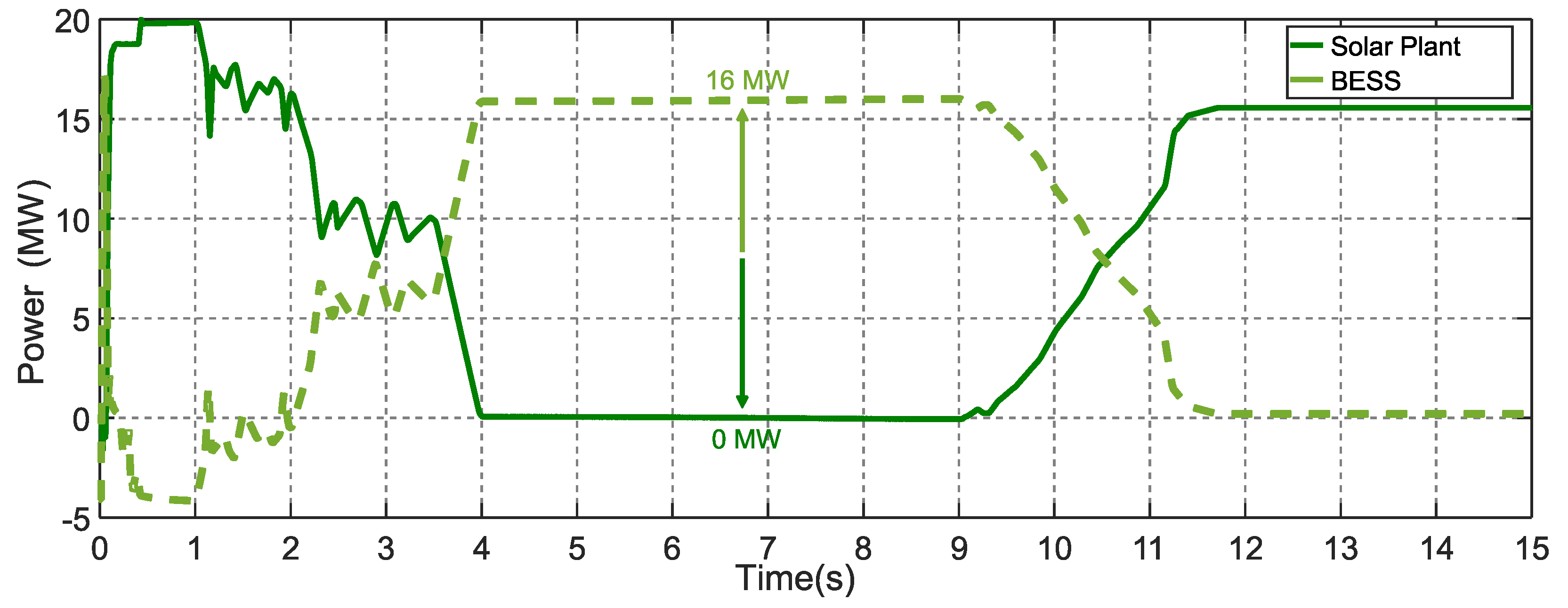
• Design, control, and coupling of BESS to the solar plant, contributing to smoothing the power delivered to the grid and minimizing the operational uncertainties.

2. Proposed Modeling for Transient Analysis

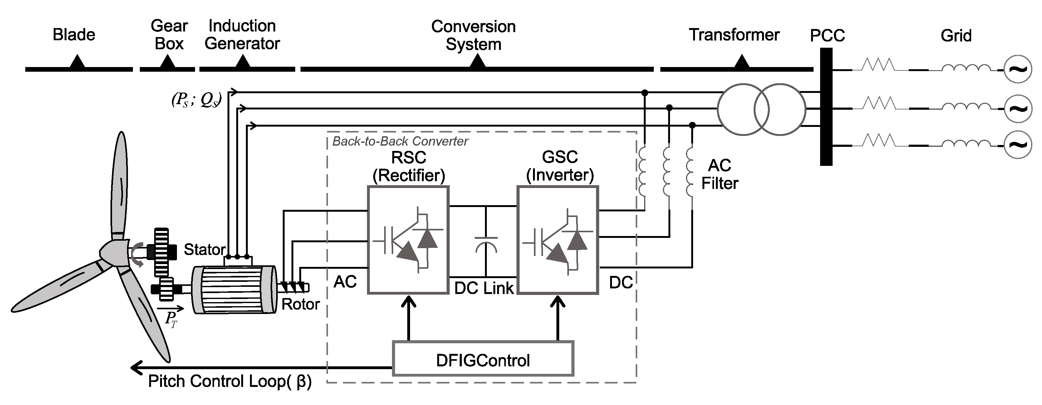
2.1. Wind Power Plant

Among the different types of generators used in the wind energy conversion system, the DFIG, illustrated in Figure 1, is the most applied today, having dominance in the market and being selected for this work. The control contained in these wind turbines seeks to operate in maximum power point tracking (MPPT) for each wind speed [39]. In addition, it stands out for its many advantages related to the technical and economic aspects [40,41].

The DFIG consists of a wound rotor induction generator connected to the turbine through a gearbox [39]. In this technology, the stator windings are directly connected to the three-phase grid and the rotor windings are directly connected to a converter. In this work, a back-to-back converter composed of a rotor-side converter (RSC) and a grid-side converter (GSC) was used [39,42]. The GSC acts to keep the voltage on the DC link constant, generating or absorbing reactive power. The RSC controls the flow of active and reactive power, making it possible to operate the turbine in the MPPT.

Among the various DFIG control modes found in the literature, the strategy employed in this work used voltage-oriented vector control (VOC) [42,43]. Among its many advantages, this control allows a simplified representation of the variables of the electric generator (given in three-phase coordinates $abc$) from two-phase coordinates $dq$ [39]. In the $dq$ reference frame, magnitude decoupling is possible, which results in independent control of active (P) and reactive (Q) power [43].

For a complete understanding, mathematical equations and further explanations can be found in [39,40,41,42,43,44].

2.2. Solar Power Plant

The topology for modeling the PV generation plant was composed of three elementary parts, as illustrated in Figure 2. The output terminals of the PV array were connected to a DC/DC converter of boost topology to stabilize the voltage and maintain the system in the MPPT [45,46]. In the control strategy of this converter, the power output of the PV array was compared with a reference signal from the MPPT and then fed to a PI (proportional integral) controller, which generates the duty cycle and the switching for the converter [47]. In this work, the MPPT algorithm applied featured incremental conductance with integral regulation [48]. The classical technique is based on the principle of perturbation and observation, being easy to implement with good performance in the steady state and with a quick response to changes in irradiance. Lastly, the output of the converter is connected to an electronic DC/AC power inverter, with a VOC-based control strategy, similar to the one described in Section 2.1 (where the $\mathrm{d}$ axis, from the synchronous reference, is aligned with the mains voltage vector) [42,45,46,47,48].

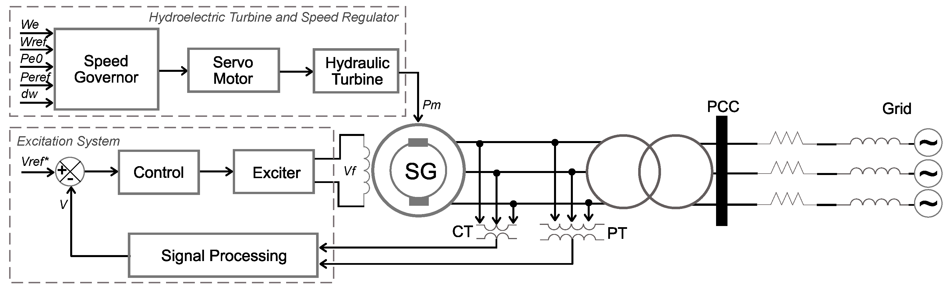
2.3. Hydroelectric Power Plant

Even today, much of the electrical energy generated worldwide comes from synchronous, thermal, or hydraulic machines that can operate in parallel with the grid [49,50]. They have a significant moment of inertia and many attributes favorable to EPS considering transient stability and reliability [26]. Therefore, a hydroelectric plant with a salient pole synchronous generator was considered, as shown in Figure 3.

The input and output variables of the excitation system are $V_{ref}{}^{*}$ the reference value of the stator terminal voltage and $V_f$ the field voltage for the generator. The turbine and speed governor inputs are $W_e$ the actual machine speed, $W_{ref}$ the reference speed, $P{e}_0$ the nominal electrical power of the machine, ${Pe}_{ref}$ the mechanical reference power, and $d_w$ the speed deviation. The inputs are processed by a PID controller (proportional, integral, derivative), which produces the generator’s output signal ($P_m$), representing controlled mechanical power.

The synchronous machine model considered the dynamics of the stator windings, field, and dampers. Similar to the one presented in Section 2.1, the $\mathrm{dq}$ synchronous reference was applied to conceptualize the equivalent circuit and equate the machine. The rotor parameters and the electrical quantities were analyzed from the stator in this representation.

The turbine and speed governor modeling was based on the document “Hydraulic Turbine and Turbine Control Models for Dynamic Studies” found in [51,52]. This model was chosen by the level of maturity, being very useful in studies such as the one proposed.

The excitation system was implemented as the type 1 model established by [53]. In this system, the generator terminal voltage ($V_f$) is adjusted through a controller where the comparison of the input signals generates an error that is changed. Finally, the signal is used in the exciter that operates in the established range. More details about the excitation system, its working principle, and control theory can be found in [51,53].

2.4. Transmission Grid

2.4.1. Lines, Transformers, and Loads

The transmission lines were represented by the π model (concentrated) in a similar way to the practices adopted in electromechanical transient stability studies since it has reduced computational effort and satisfactory accuracy [3,54]. Contrary to the distributed parameter line model where resistance, inductance, and capacitance are uniformly distributed along the line, the π model groups the line parameters into a single section [3].

The transformers used in this study were represented by the classic two-winding model [55]. The model considers winding resistances ($R_1$ and $R_2$), leakage inductances ($L_1$ and $L_2$), and core magnetization characteristics ($R_m$ and $L_m$), where losses are considered, but saturation characteristics are not considered [55].

The loads were represented by three-phase dynamic models expressing the active and reactive power consumed over time, varying as a function of the magnitude of the positive sequence voltage of the buses. The premise has been established that load currents are balanced even under voltage unbalance conditions [3,56]. The active ($P_L$) and reactive ($Q_L$) power of the loads are considered separately, and the voltage dependence is given by exponential functions [3].

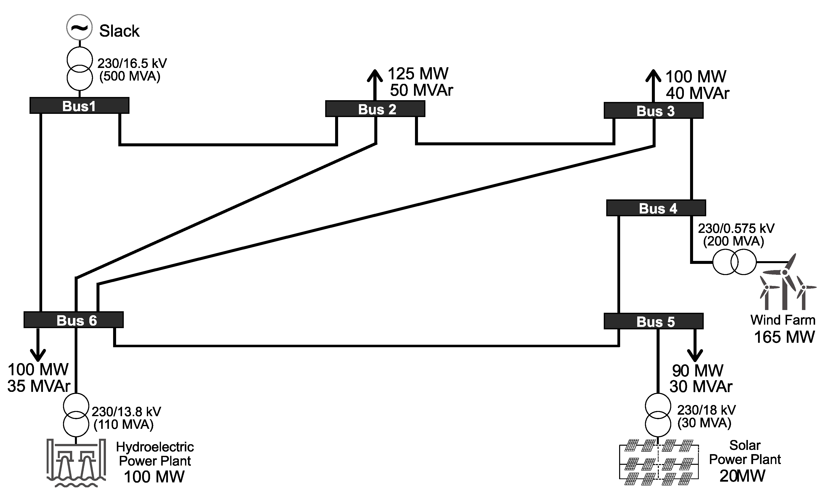
2.4.2. Test Transmission Grid

The single-line model diagram is illustrated in Figure 4 and represents a transmission grid that operates at high voltage (230 kV), defined in Brazil as the primary or basic grid. Although it is a relatively small model compared to other systems also used, it allowed the application of all the concepts proposed by the present work [50].

The test grid was obtained by adapting the famous Western System Coordinating Council (WSCC), usually discussed in the literature [1,25,49,50], with parameters obtained from [57]. The system consists of six buses, eight lines, and three generation sources, with bus 1 being the reference bus (slack). Adaptations were carried out to make the proposed studies viable, highlighting the addition of the wind power plant (165 MW), the solar PV plant (20 MW), and the hydroelectric plant (100 MW).

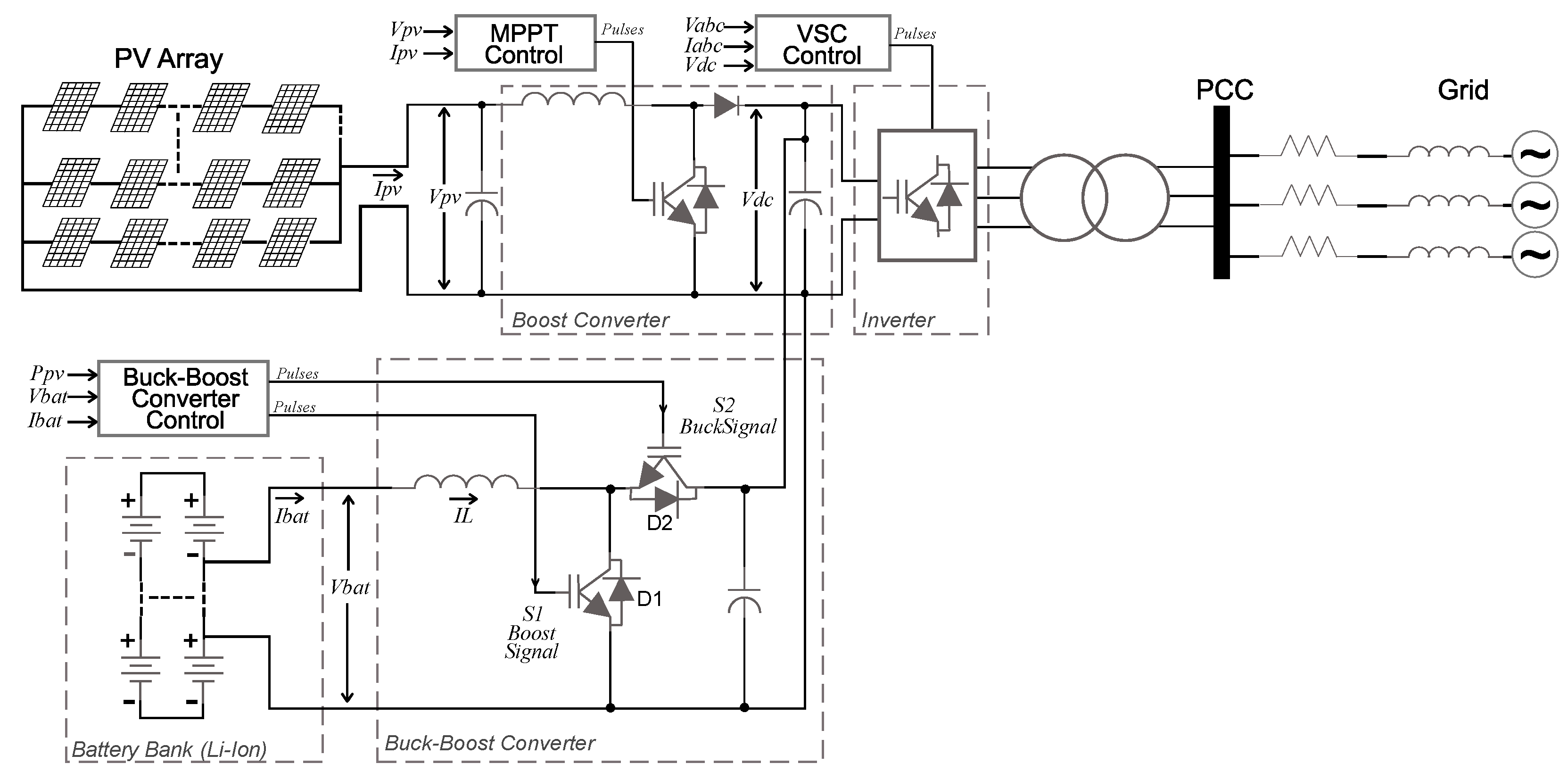
3. Proposal for Coupling BESS to the Solar PV Plant

Solar PV generation is subject to weather conditions such as passing clouds and sudden weather changes, which causes uncertainties and sudden variations in generation [47,58]. For this reason, when the penetration of this source in the EPS is high, the oscillation in the generation can cause the loss of large blocks of power, implying impacts on the transient stability [47].

For the reasons explained, a BESS was designed to smooth the solar plant output, aiming to mitigate the variation in the power delivered to the grid and eliminate sudden drops in energy generation. The coupling of the BESS with the power plant is illustrated in Figure 5 and was carried out by integrating three components: battery bank, bidirectional DC/DC buck–boost converter, and control unit.

A lithium ion (Li-ion) battery was chosen because it is the technology with the most significant application in EPS, according to IEA data [12]. Some advantages are its composition of sealed cells that do not require maintenance, long life cycle, wide operating temperature range, fast charging, high efficiency in charge and discharge mode, high energy density, flexibility, modularity, and speedy response time (in milliseconds) [9,11,13].

3.1. Modeling the Lithium-Ion Battery Bank

The modeling of the batteries was carried out using the model presented by Tremblay et al. [59]. This model can accurately represent the characteristic curves of electrochemical batteries when compared with the manufacturer datasheet [60,61]. According to tests, the accuracy for the lithium battery corresponded to a margin of error of ±3% [59]. The mathematical model is given by different equations for charge and discharge [62].

$$V_{bat}=V_0-K\frac{Q}{it+0.1\cdot Q}{i}^{*}-K\frac{Q}{Q-it}it+A\mathit{exp}\left(-Bit\right),$$

(1)

$$V_{bat}=V_0-K\frac{Q}{Q-it}{i}^{*}-K\frac{Q}{Q-it}it+A\mathit{exp}\left(-Bit\right),$$

(2)

where $V_{bat}$ is the battery voltage, $V_0$ is the voltage constant (V), $v$ is the polarization constant, $Q$ is the battery capacity, $it$ is the capacity extracted, $i^{*}$ is the filtered reference current, $A$ is the exponential voltage zone, and $B$ is the exponential capacity.

The battery state of charge (SOC) (which ranges from 0 to 100%) is given by

$$SOC=100\left(1-\frac{1}{Q}{\int }_0^{t}i\left(t\right) dt\right).$$

(3)

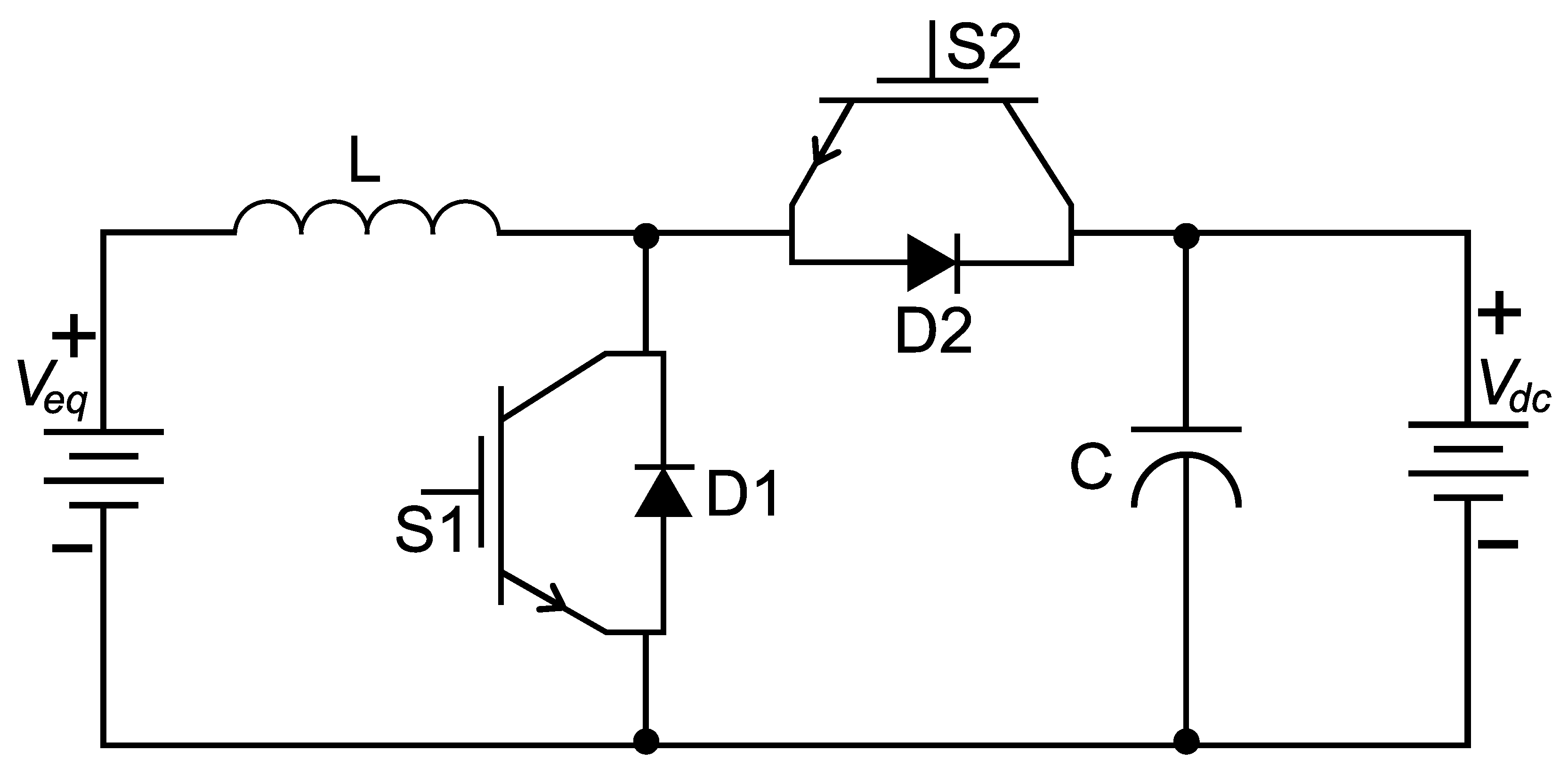
3.2. Bidirectional Buck–Boost Converter

The converter topology employed is illustrated in Figure 6, which allows current and power to flow from the battery to the DC link and vice versa, ensuring the reversal of power flow between the two systems as needed [45,60].

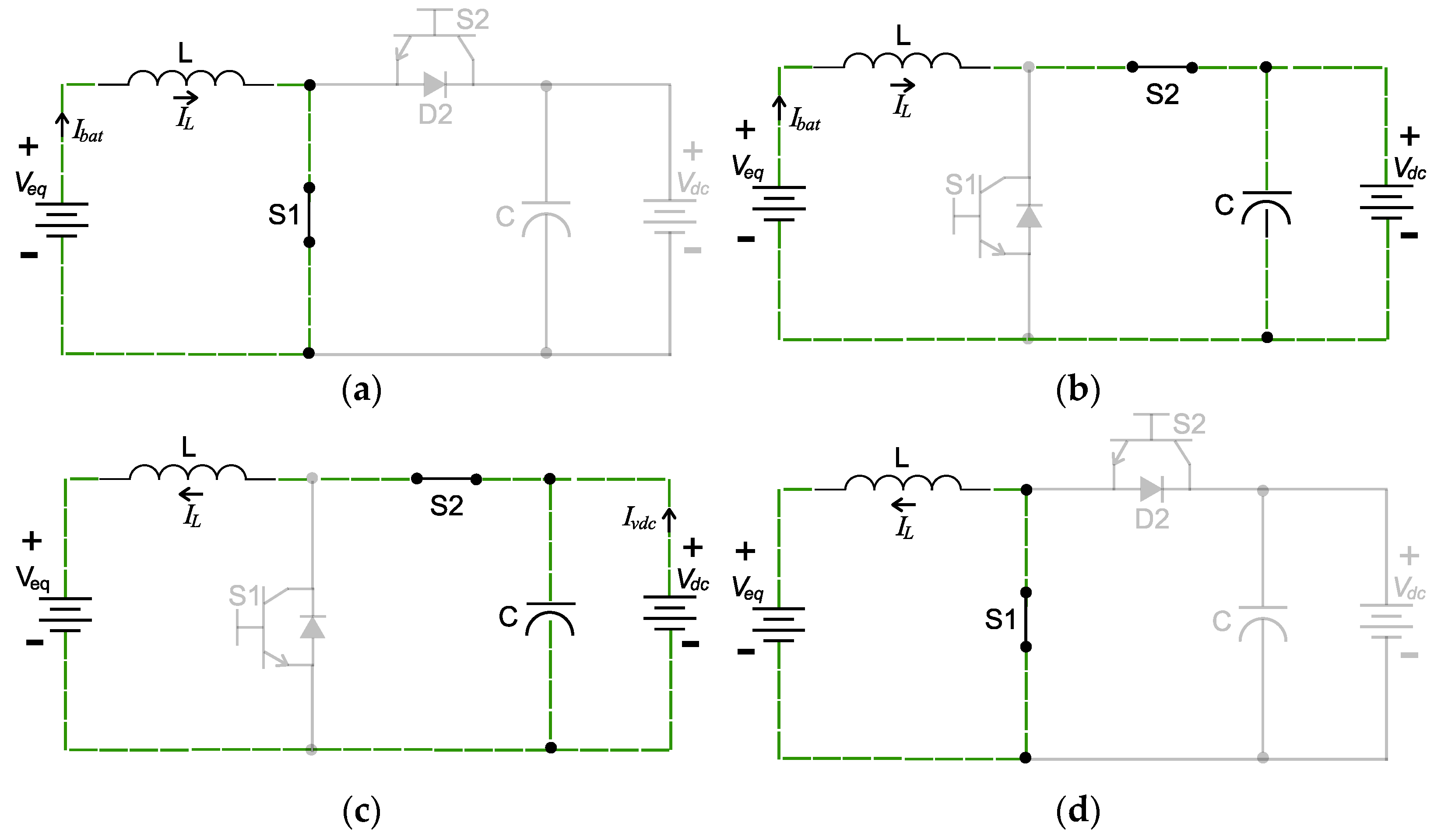
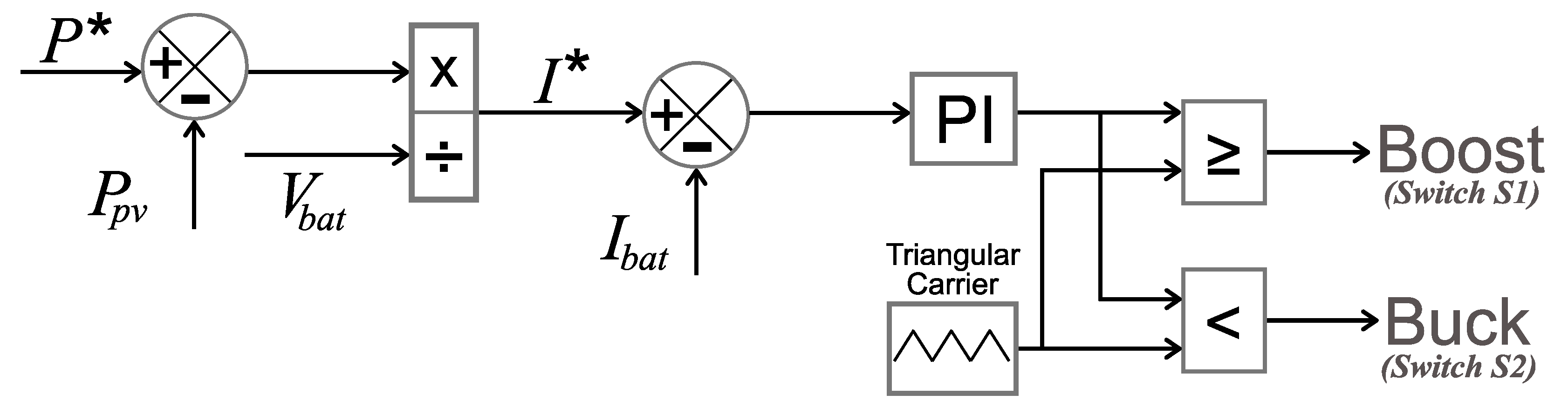
3.2.1. Converter Switching and Control Strategy

The management of the charging and discharging stages of the battery bank takes place by controlling the current flowing through the inductor $L$ (Figure 6). The converter must operate in continuous conduction mode, acting in two stages since the current flowing through the circuit can be positive or negative. For this, the switch $S1$ is controlled in a complementary way to $S2$, and they never operate simultaneously. Their activation is performed by a train of PWM pulses, causing the switches to turn on in the first subinterval and turn off in the following subinterval [45].

In the considered system, the DC link voltage of the PV plant is higher than the BESS voltage. Thus, the converter acts in buck mode in the charging process, lowering the voltage to the BESS level. Otherwise, in the discharge process, the converter operates in boost mode, raising the voltage level to the nominal value of the DC link. The details of these two stages are presented in Figure 7.

The operating steps of this converter were similarly addressed by [63] and can be described as follows:

• Stage 1 (discharge, boost), power flow from the battery bank ($V_{eq}$) to the DC link ($V_{dc}$): When switch $S1$ is on, the diode $D2$ is reverse-polarized, and then the batteries deliver current to inductor $L$ (Figure 7a). When switch $S2$ is on, the diode $D1$ is reverse-polarized, and inductor S1 supplies power to the DC link (Figure 7b).
• Stage 2 (load, buck), power flow from the DC link ($V_{dc}$) to the battery bank ($V_{eq}$): When switch $S2$ is on, diode $D1$ is reverse-polarized, and the DC link supplies current to inductor $L$ (Figure 7c). When switch $S1$ is on, diode $D2$ is reverse-polarized, and the inductor L delivers power to the batteries (Figure 7d).

The converter, battery, and control set must manage the power delivered to the grid. For this, the converter operates in buck mode (charging the battery) at power levels above the established reference. On the other hand, the converter operates in boost mode for power below the reference, discharging the battery to maintain the power level at the reference as proposed in [64]. The adopted control strategy is illustrated in Figure 8.

The reference power $P^{*}$ is compared with the active power ($P_{pv}$) produced by the PV array [65], generating a signal that is divided by the value of the battery voltage ($V_{bat}$) and producing the current reference $I^{*}$. It is compared to the battery current ($I_{bat}$) and processed by the PI controller. The result is compared to a 12 kHz constant frequency triangular producing the pulses for switches $S1$ (boost signal) and $S2$ (buck signal). A better understanding can be obtained by analyzing in Figure 7 together. In this control strategy, the logic is established by Equation (4).

$$\{\begin{array}{c}if P^{*}>P_{pv}, the battery is charged, absorbing energy from the DC link;\\ if P^{*}\le P_{pv}, the battery is discharged, injecting energy into the DC link.\end{array}$$

(4)

4. Tests and Results

4.1. Electromechanical Stability Analysis: Initial Guidelines and Assumptions

The simulations were proposed in the time domain considering the transmission system illustrated in Figure 4. All grid components, including alternating current generators, wind power plant, solar power plant, transformers, and loads, were represented by detailed three-phase models, and the parameters used are available in Appendix A. Modeling and simulations were performed with Matlab^® and Simulink^® software [66]. Some guidelines and assumptions are presented below.

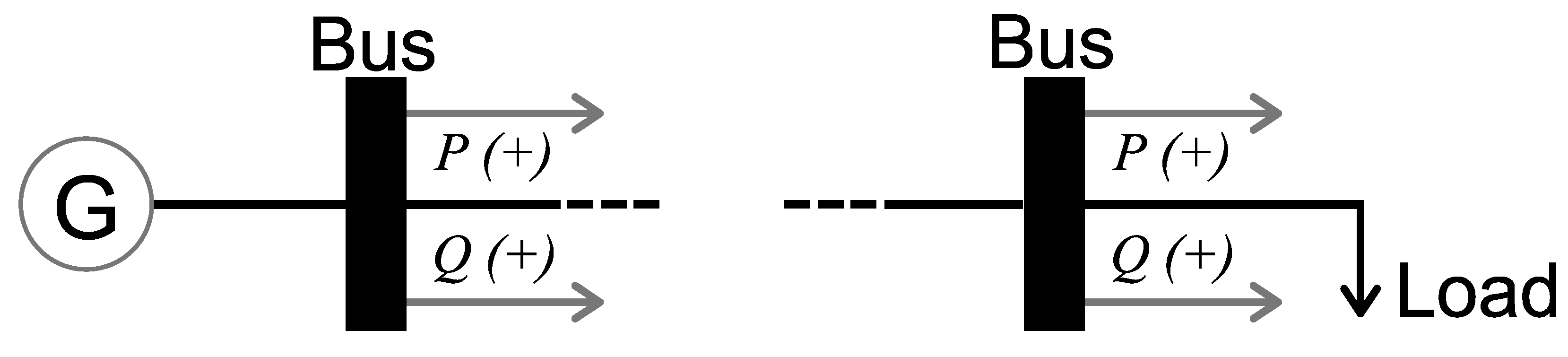
• The analyses were conducted on the basis of the current Brazilian grid code, Grid Proceedings [38]. The main tables and figures used for the analysis are in Appendix B, and the sign convention is illustrated in Figure 9;
• According to guidelines for electrical studies obtained, all simulations were performed under a time horizon of 15 s (using an initial state vector to start the system in the steady state) [38];
• In the variables calculated and presented in pu (values per unit), the base power was 100 MW, and the base voltage was equal to the rated voltage of the bus itself;
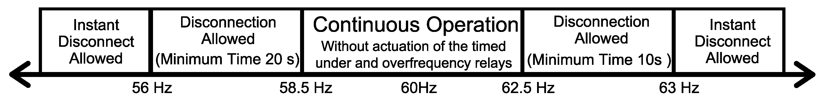
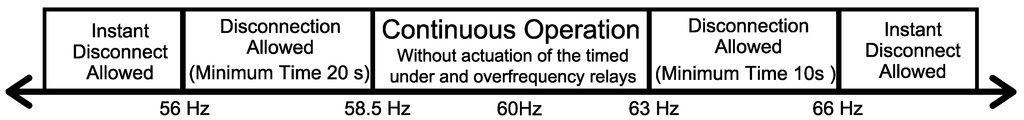
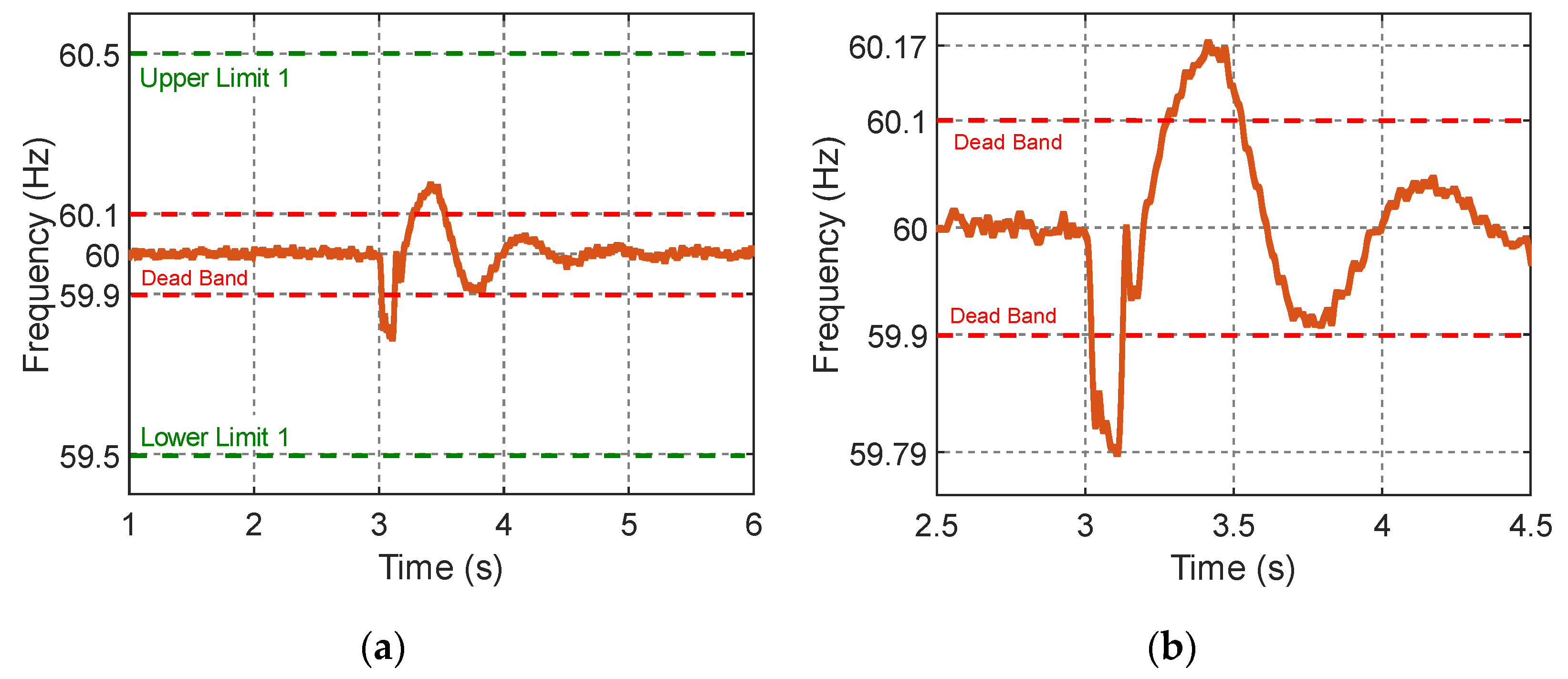
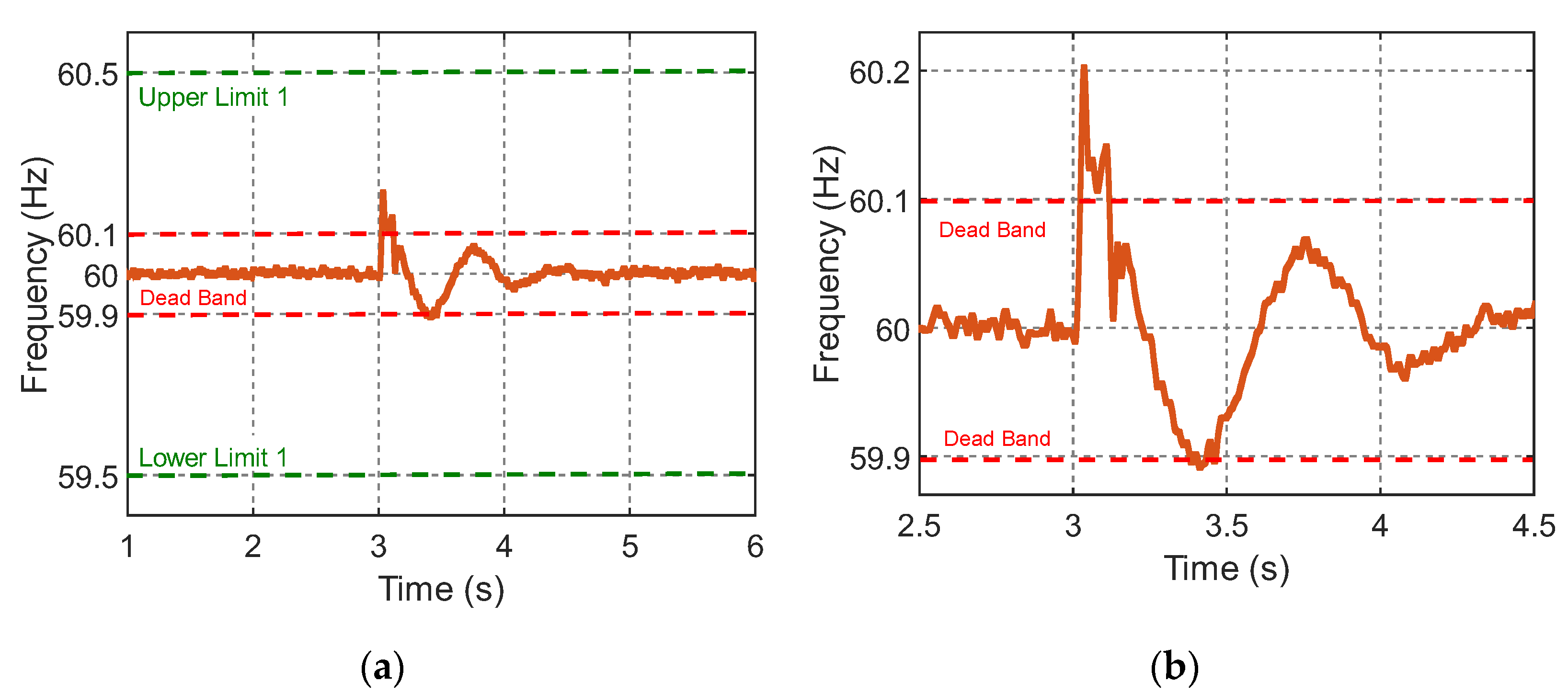
• The Brazilian standard frequency is 60 Hz where, as established in [38], under normal conditions (permanent regime, without the occurrence of disturbances), it should not exceed ±0.1 Hz. Its means that deviations from the nominal regime frequency must be within the limits of 59.9 Hz to 60.1 Hz. The literature defines as steady-state oscillation dead zone or dead band [4];
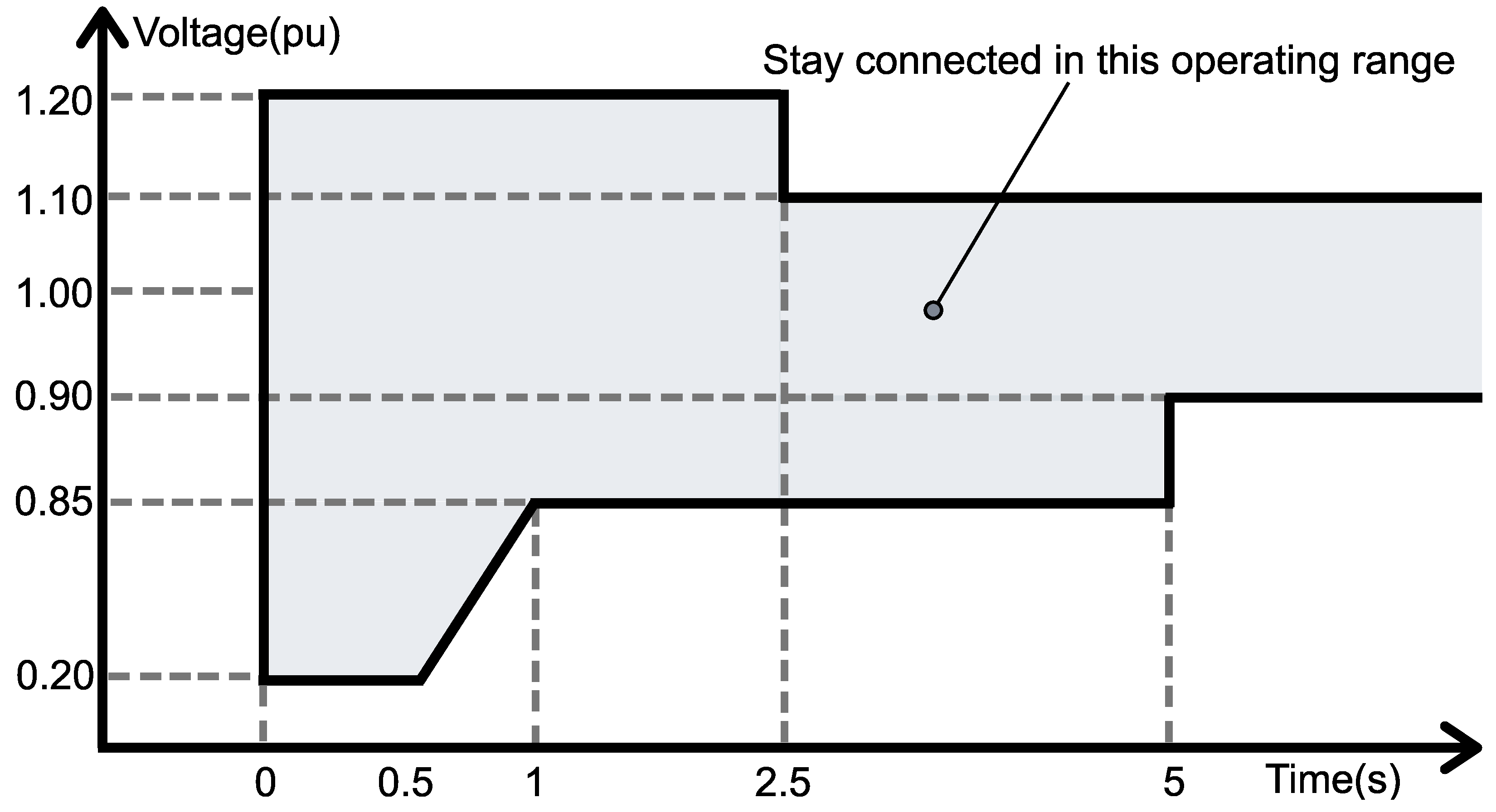
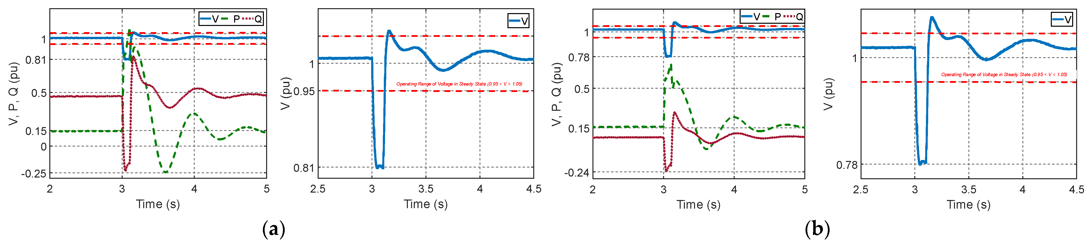
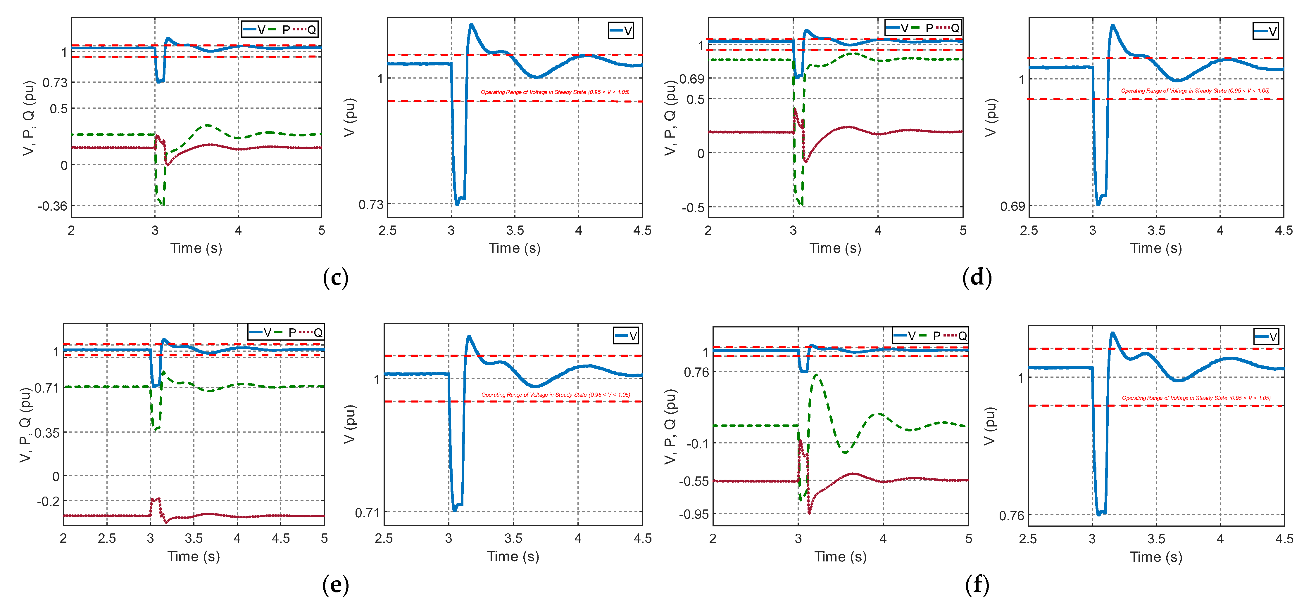
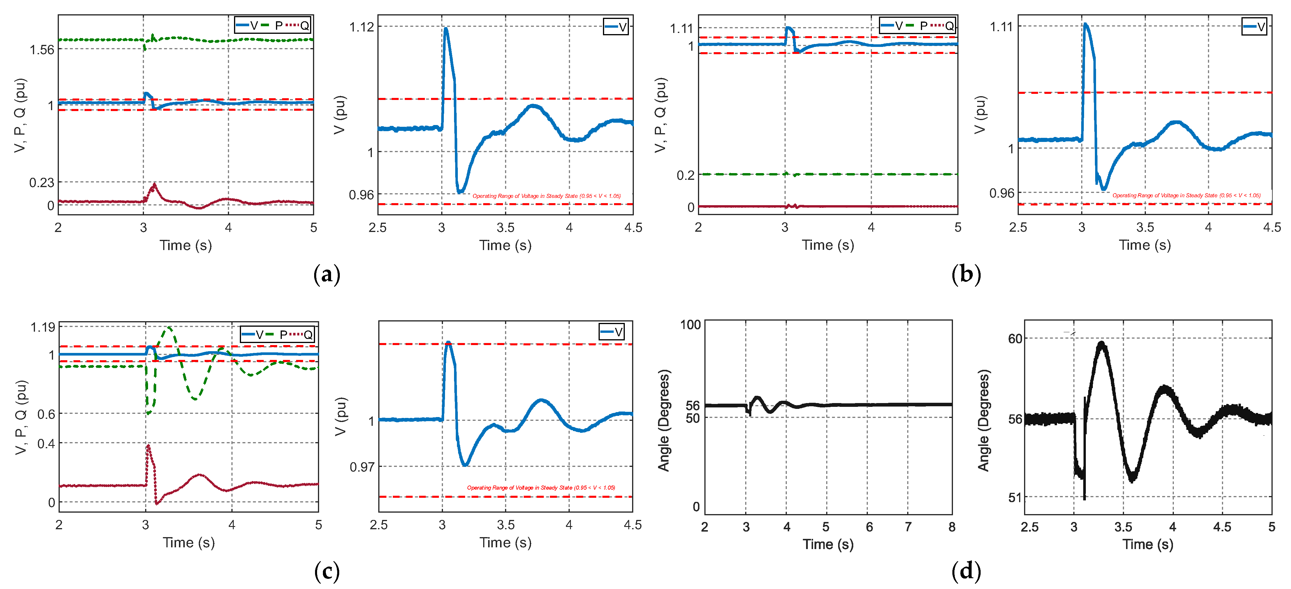
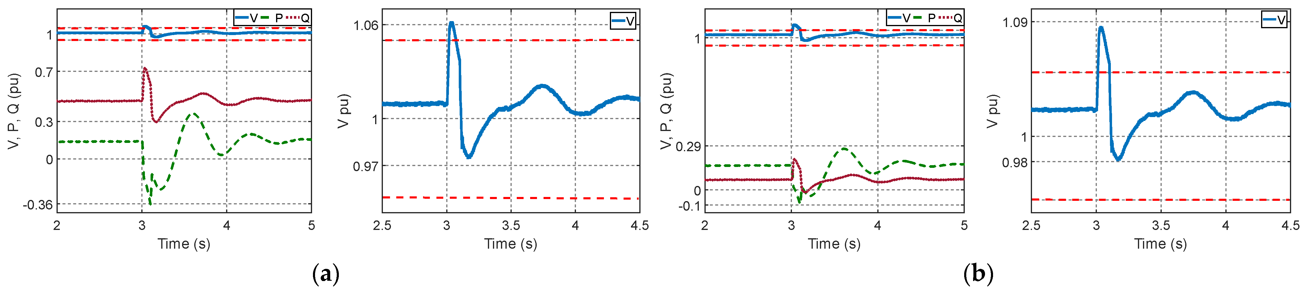
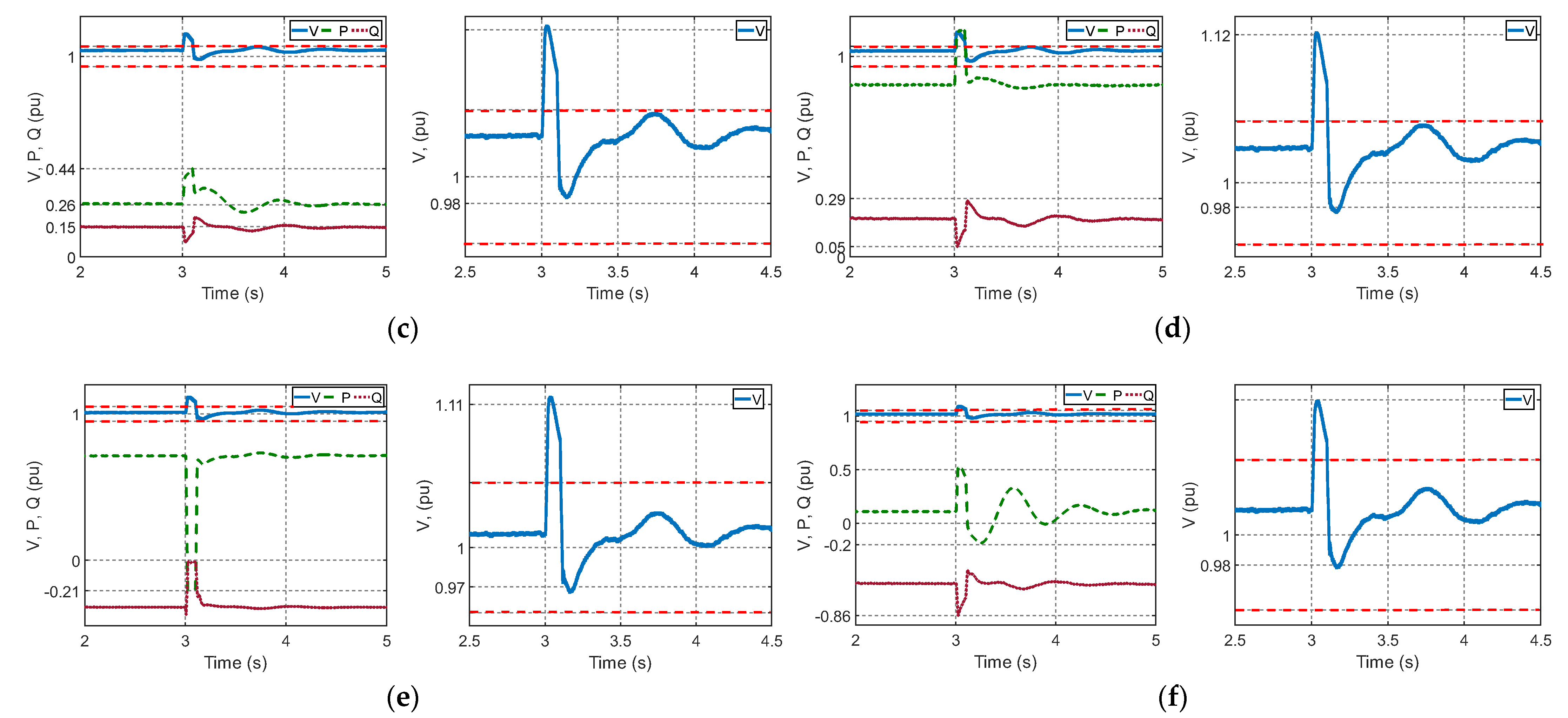
• Regarding voltage, the operating limit in the steady state is understood by the ratio 0.95 < V < 1.05, and the generators need to operate in this range without being turned off [38]. To this end, the graphs contain a red dotted line showing the upper (1.05) and lower (0.95) limits;
• The scenarios were designed to cover different operating conditions of the EPS, following the preoperational studies required by the ONS to request access to the grid commissioning, among others [38].

4.2. Scenario 1: Three-Phase Fault at Wind Power Plant Terminals

In the first scenario, one symmetrical and balanced three-phase fault involving earth occurred at the wind power plant terminals (Bus 4, Figure 4). The event was transient, starting at 3 s and ending at 3.1 s (duration 100 ms).

As used in studies of transient stability in significant disturbances, variations in wind speed (wind plant), irradiance and temperature values (solar plant), and inflow (hydroelectric plant) were not considered [67]. All generating units continued to deliver their rated active power to the grid, with the reactive power adjusted to 0 Mvar (unit power factor).

In the wind farm, the wind speed was constant at 15 m/s (speed relative to the extraction of rated power), with the pitch angle of the turbines set at 8.7° and the generator speed at 1.2 pu. The irradiance and temperature values of the solar plant were 1000 W/m² and 25 °C, respectively.

4.2.1. Generators Analysis

In the wind farm (Figure 10a), the solar plant (Figure 10b), and the hydroelectric plant (Figure 10c), the occurrence of short-term voltage variations (STVVs) can be noticed according to

Table A11. Short-term voltage variations (STVV).

Type of STVV	Duration of STVV	Amplitude of STVV Concerning the Rated Voltage (ARV)
Momentary voltage interruption (MVI)	≤3 s	ARV < 0.1 pu
Momentary voltage sag (MVS)	≥1 cycle and ≤3 s	0.1 ≤ ARV < 0.9 pu
Momentary voltage rise (MVR)	≥1 cycle and ≤3 s	ARV > 1.1 pu
Temporary voltage interruption (TVI)	>3 s and ≤1 min	ARV < 0.1 pu
Temporary voltage sag (TVS)	>3 s and ≤1 min	0.1 ≤ ARV < 0.9 pu
Temporary voltage rise (TVR)	>3 s and ≤1 min	ARV > 1.1 pu

(Appendix B). The Brazilian operator classifies this disturbance as a momentary voltage sag (MVS), where the voltage value is between 0.1 and 0.9 pu for an interval ≥1 cycle and ≤3 s [38]. In the proposed graphs, the red dotted line shows the upper and lower limits within which the voltage must remain in a steady state (0.95 < V < 1.05).

As expected, the greater MVS occurred at the wind farm, given its proximity to the fault point. All generators returned to the steady-state condition within about 2 s of the disturbance. As regulated by Brazilian grid codes, wind and solar generation must avoid shutdown due to voltage instability, operating within limits established by the LVRT curve observed in Figure A2 (Appendix B). All voltage curves remained within the permitted zones, and none of the generating plants were shut down. The load angle of the synchronous generator, illustrated in Figure 10d, oscillated; however, it returned to the original pre-fault position, indicating angular stability.

4.2.2. Bus and System Frequency Analysis

Results relative to system buses are shown in Figure 11. As with the generators (Section 4.2.1), there was severe MVS, but with a magnitude and duration shorter than the time of action of the protection system, which would lead to service interruption [38]. The most expressive MVS occurred in the buses closest to the short circuit, justified by the influence of the impedances of the transmission lines. All analyzed variables returned to the normal condition in about 2 s (120 cycles at a frequency of 60 Hz), soon after the extinction of the fault, after a short oscillatory regime. In conclusion, the system appeared to be robust, behaving stably.

Lastly, the system frequency is shown in Figure 12, where it is noted that the severity of the fault did not impose significant disruptions to the system. The frequency amplitude exceeded the dead band limits by 0.12% (above) and 0.18% (below). The frequency variation did not exceed the limitations of the buses (

Table A10. System frequency limits in case of perturbation.

Frequency Range (Hz)	Maximum Exposure Time (s)
f > 66.0 Hz	0
63.5 Hz < f ≤ 66.0 Hz	30
62.0 Hz < f ≤ 63.5 Hz	150
60.5 Hz < f ≤ 62.0 Hz	270
58.5 Hz ≤ f < 59.5 Hz	390
57.5 Hz ≤ f < 58.5 Hz	45
56.5 Hz ≤ f < 57.5 Hz	15
f < 56.5 Hz	0

, Appendix B) or the operating requirements of the generators (Figure A1 and Figure A2, Appendix B).

4.3. Scenario 2: Load Rejection at Bus 5

The load localized at bus 5 (Figure 4) was temporarily disconnected from the system. Switching occurred at 3 s with a duration of 100 ms. The generation kept up to the same standards described in scenario 1 (Section 4.2). The load removed from the system corresponds to approximately 23% of the loading level, and its participation in the energetic balance is quite significant. Albeit at a lower intensity than recorded in the first scenario, there was a critical disturbance event in the system.

4.3.1. Generators Analysis

In the wind farm (Figure 13a) and solar plant (Figure 13b), there was a momentary voltage rise (MVR): variation in which the amplitude concerning the rated voltage is greater than 0.1 pu, with an interval ≥1 cycle and ≤3 s (Table A11, Appendix B) [38]. In the hydroelectric plant (Figure 13c), the level of variation is not expressive, not exceeding the limits of steady states. The load angle of the synchronous generator (Figure 13d) quickly stabilized, returning to the original position. The magnitude of the fault did not impose large disturbances to the point of compromising the normal operating levels of the generators as established in the LVRT curve (Figure A3) [38]. In the proposed graphs, the red dotted line shows the upper and lower limits within which the voltage must remain when in a steady state (0.95 < V < 1.05).

4.3.2. Bus and System Frequency Analysis

The results for the system buses are illustrated in Figure 14. The impacts of the load output were reflected in the system, with the MVR observed in all buses [38]. However, the severity and duration would not result in sudden activation of the protection system (not considered in this work). The system returned to steady state in 2 s (120 cycles at 60 Hz), showing electromechanical stability.

The system frequency (Figure 15) was also impacted but with a lower degree of compromise compared to the occurrence of a three-phase fault. The amplitude of the variation extrapolated the dead band limits, but not aggressively. The frequency stabilized in about 2 s, showing that the system has stability for load shedding cases.

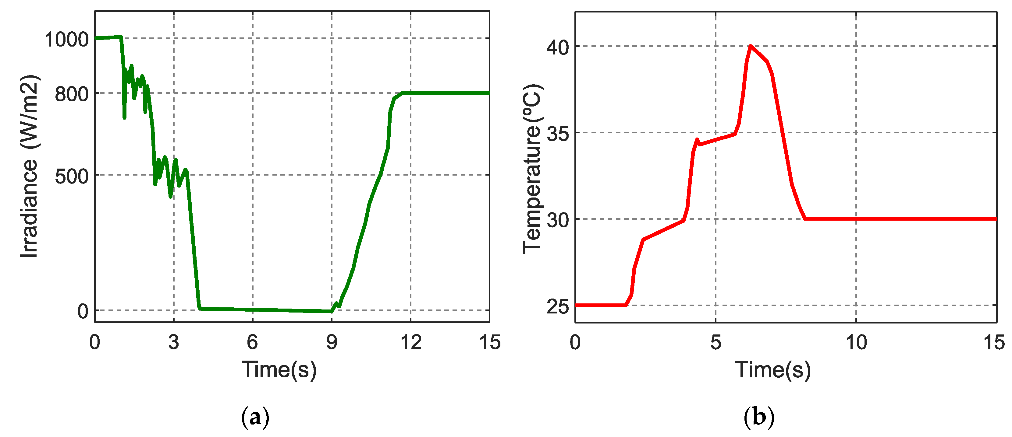
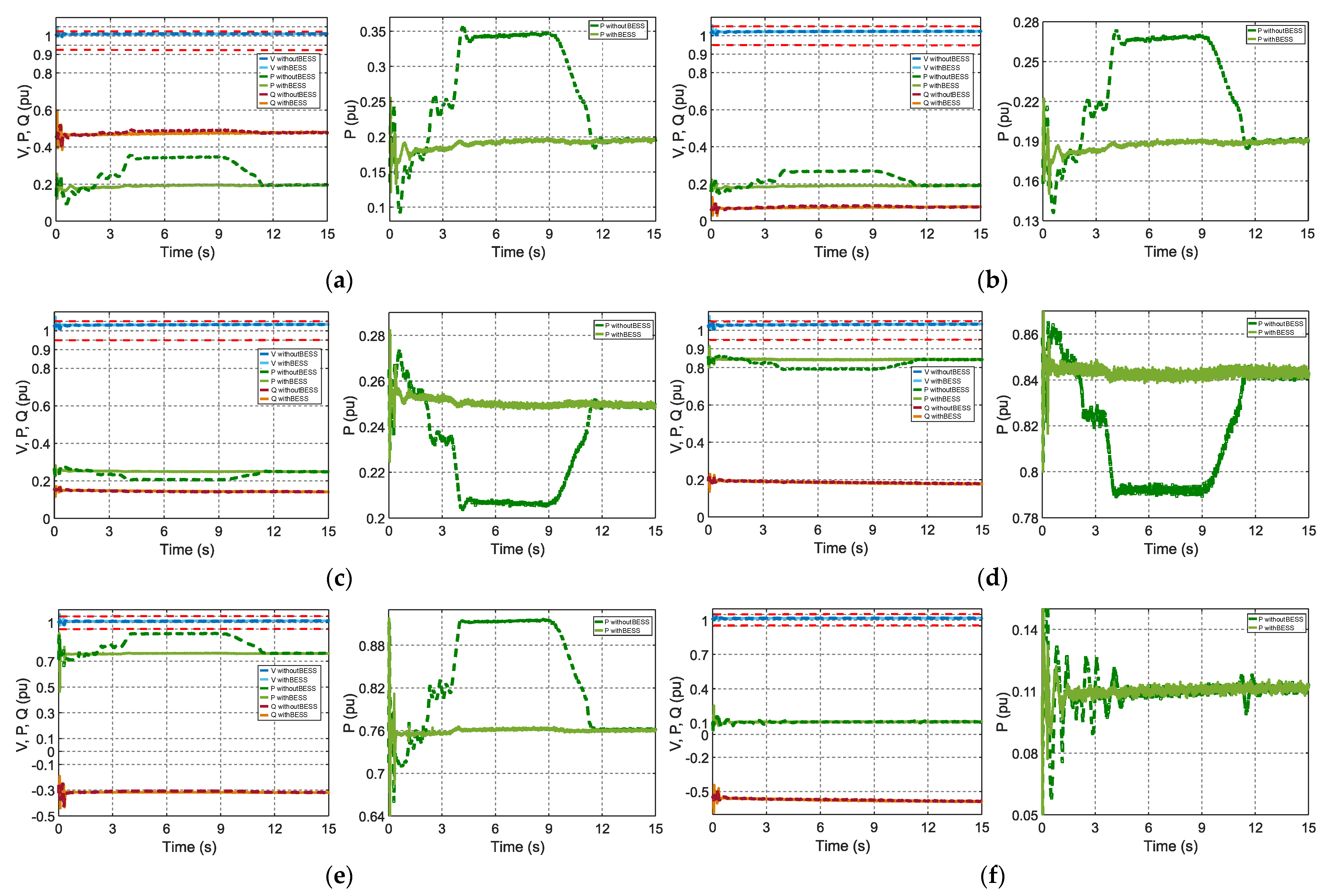
4.4. Scenario 3: Power Variation at the Solar Power Plant and BESS Performance

Lastly, tests related to the integration of BESS to the solar plant were carried out. The reference of the control $P^{*}$ (Section 3.2.1) was adjusted to deliver a constant power of 16 MW, regardless of fluctuations in the PV generation. In this configuration, BESS has an autonomy of 3 h. Additionally, BESS can support PV system failure events, including moments of complete generation loss. The generation of wind and hydroelectric plants remained constant. The irradiance and temperature curves shown in Figure 16 were used in the solar plant. As illustrated, from 0 to 4 s, there was considerable variation, and the generation was entirely zeroed between 4 and 9 s. This situation simulates the effect of full shading of the plant, which implies the complete loss of power delivered to the grid. After 9 s, the irradiance recovered growth, stabilizing at 800 W/m².

4.4.1. Solar Plant in Conjunction with BESS Analysis

In the graph presented in Figure 17, the power curves of the solar plant and BESS were plotted simultaneously. Note that the solar plant completely lost its generation between 4 and 9 s, as shown in the graph. During this period, it is observed that the power curve delivered by BESS was complementary to the curve of the solar plant. When the solar plant completely lost its generation, BESS injected the energy necessary to maintain the power delivered at the reference level (16 MW). In this way, the storage system mitigated power variations in power outages.

Figure 18 illustrates the behavior of the variables evaluated comparing two cases: with and without BESS. Regarding voltage, no variations were noticed that could compromise the standardized indices [38]. Concerning the power, the smoothing promoted by BESS brought gains to the system since it kept the flow of energy delivered to the grid constant, contributing to its stability and reliability.

4.4.2. Bus and System Frequency Analysis

The results for the system buses are illustrated in Figure 19. For both cases (with and without BESS), all the system buses kept their voltage level within normal conditions (0.95 < V < 1.05, red dotted line in graphs) [38].

It is essential to emphasize the behavior of the active power variation in all the buses. It can be seen that the BESS coupled to the solar plant could act by mitigating the fluctuations in the active power of the solar plant, replicating the benefit of power smoothing for all the other system buses. BESS’s additional active energy support improved energy export flows, making the system more stable, reliable, and robust.

5. Conclusions

The present work produced a dynamic analysis study through computational modeling and simulation, focusing on electromechanical stability. Three scenarios in a transmission system with significant penetration of wind, solar, and hydraulic generating plants were composed and analyzed according to the Brazilian grid code [38]. The coupling of BESS was also carried out as an alternative to attenuate power fluctuations/variations in the solar generation unit.

The results were encouraging, verifying that the penetration of intermittent sources in the considered transmission system did not compromise the standardized limits and did not bring risks to the transitory stability. This shows that relatively high penetration levels can be achieved, provided that the due studies are validated.

Like other analysis techniques, as proposed in [21], electromechanical stability analysis is a tool that can help evaluate the performance of the electrical grid with the wide application of renewable sources. The results obtained to the proposed system showed good performance in the joint operation between renewables and the high-voltage transmission grid. Additionally, the application of BESS shows promise for energy fluctuations. However, this solution may not be technically or economically viable for any grids. In some cases, the analysis can achieve results that demonstrate the need for a specific solution.

The present is marked by the improvement of technology related to storage systems, being an opportune moment for applications on a utility scale, primarily to mitigate the adverse effects of renewables and provision of ancillary services [12]. This improvement has technical and economic characteristics, generally associated with increased energy density and price reduction [9]. As the new sources comply with the technical requirements of connection to the power grid, their expansion in the system is guaranteed. Thus, modernization and the energy transition become possible starting from technical premises.

References

1. Sauer, P.W.; Pai, M.A.; Chow, J.H. Power System Dynamics and Stability: With Synchrophasor Measurement and Power System Toolbox, 2nd ed.; John Wiley & Sons, Ltd.: Chichester, UK, 2017; ISBN 9781119355755. [Google Scholar]
2. Venkataraman, S.; Ziesler, C.; Johnson, P.; Van Kempen, S. Integrated Wind, Solar, and Energy Storage: Designing Plants with a Better Generation Profile and Lower Overall Cost. IEEE Power Energy Mag. 2018, 16, 74–83. [Google Scholar] [CrossRef]
3. Kundur, P. Power System Stability and Control, 1st ed.; McGraw-Hill Inc.: New York, NY, USA, 1994; ISBN 007035958. [Google Scholar]
4. Attya, A.B.; Dominguez-Garcia, J.L.; Anaya-Lara, O. A review on frequency support provision by wind power plants: Current and future challenges. Renew. Sustain. Energy Rev. 2018, 81, 2071–2087. [Google Scholar] [CrossRef] [Green Version]
5. Ullah, K.; Basit, A.; Ullah, Z.; Aslam, S.; Herodotou, H. Automatic Generation Control Strategies in Conventional and Modern Power Systems: A Comprehensive Overview. Energies 2021, 14, 2376. [Google Scholar] [CrossRef]
6. Rahman, M.J.; Tafticht, T.; Doumbia, M.L.; Mutombo, N.M.-A. Dynamic Stability of Wind Power Flow and Network Frequency for a High Penetration Wind-Based Energy Storage System Using Fuzzy Logic Controller. Energies 2021, 14, 4111. [Google Scholar] [CrossRef]
7. Asiaban, S.; Kayedpour, N.; Samani, A.E.; Bozalakov, D.; De Kooning, J.D.M.; Crevecoeur, G.; Vandevelde, L. Wind and Solar Intermittency and the Associated Integration Challenges: A Comprehensive Review including the Status in the Belgian Power System. Energies 2021, 14, 2630. [Google Scholar] [CrossRef]
8. Dreidy, M.; Mokhlis, H.; Mekhilef, S. Inertia response and frequency control techniques for renewable energy sources: A review. Renew. Sustain. Energy Rev. 2017, 69, 144–155. [Google Scholar] [CrossRef]
9. Robyns, B.; François, B.; Delille, G.; Saudemont, C. Energy Storage in Electric Power Grids; John Wiley & Sons, Inc.: Hoboken, NJ, USA, 2015; ISBN 9781119058724. [Google Scholar]
10. Tielens, P.; Van Hertem, D. The relevance of inertia in power systems. Renew. Sustain. Energy Rev. 2016, 55, 999–1009. [Google Scholar] [CrossRef]
11. Nadeem, F.; Hussain, S.M.S.; Tiwari, P.K.; Goswami, A.K.; Ustun, T.S. Comparative review of energy storage systems, their roles, and impacts on future power systems. IEEE Access 2019, 7, 4555–4585. [Google Scholar] [CrossRef]
12. International Energy Agency (IEA). Energy Storage Data. Available online: https://www.iea.org/fuels-and-technologies/energy-storage (accessed on 5 February 2022).
13. Dehghani-Sanij, A.R.; Tharumalingam, E.; Dusseault, M.B.; Fraser, R. Study of energy storage systems and environmental challenges of batteries. Renew. Sustain. Energy Rev. 2019, 104, 192–208. [Google Scholar] [CrossRef]
14. Wan, C.; Qian, W.; Zhao, C.; Song, Y.; Yang, G. Probabilistic Forecasting Based Sizing and Control of Hybrid Energy Storage for Wind Power Smoothing. IEEE Trans. Sustain. Energy 2021, 12, 1841–1852. [Google Scholar] [CrossRef]
15. Barelli, L.; Bidini, G.; Ciupageanu, D.A.; Micangeli, A.; Ottaviano, P.A.; Pelosi, D. Real time power management strategy for hybrid energy storage systems coupled with variable energy sources in power smoothing applications. Energy Rep. 2021, 7, 2872–2882. [Google Scholar] [CrossRef]
16. Rallabandi, V.; Akeyo, O.M.; Jewell, N.; Ionel, D.M. Incorporating battery energy storage systems into multi-MW grid connected PV systems. IEEE Trans. Ind. Appl. 2019, 55, 638–647. [Google Scholar] [CrossRef]
17. Huang, J.; Jiang, Z.; Negnevitsky, M. Ancillary Service by Tiered Energy Storage Systems. J. Energy Eng. 2022, 148, 04021059. [Google Scholar] [CrossRef]
18. Gomez, L.A.G.; Grilo, A.P.; Salles, M.B.C.; Filho, A.J.S. Combined Control of DFIG-Based Wind Turbine and Battery Energy Storage System for Frequency Response in Microgrids. Energies 2020, 13, 894. [Google Scholar] [CrossRef] [Green Version]
19. Yuan, Z.; Zecchino, A.; Cherkaoui, R.; Paolone, M. Real-Time Control of Battery Energy Storage Systems to Provide Ancillary Services Considering Voltage-Dependent Capability of DC-AC Converters. IEEE Trans. Smart Grid 2021, 12, 4164–4175. [Google Scholar] [CrossRef]
20. Mustafa, M.B.; Keatley, P.; Huang, Y.; Agbonaye, O.; Ademulegun, O.O.; Hewitt, N. Evaluation of a battery energy storage system in hospitals for arbitrage and ancillary services. J. Energy Storage 2021, 43, 103183. [Google Scholar] [CrossRef]
21. Ghiasi, M. Detailed study, multi-objective optimization, and design of an AC-DC smart microgrid with hybrid renewable energy resources. Energy 2019, 169, 496–507. [Google Scholar] [CrossRef]
22. Murty, V.V.; Kumar, A. Optimal Energy Management and Techno-economic Analysis in Microgrid with Hybrid Renewable Energy Sources. J. Mod. Power Syst. Clean Energy 2020, 8, 929–940. [Google Scholar] [CrossRef]
23. Ghiasi, M.; Esmaeilnamazi, S.; Ghiasi, R.; Fathi, M. Role of Renewable Energy Sources in Evaluating Technical and Economic Efficiency of Power Quality. Technol. Econ. Smart Grids Sustain. Energy 2020, 5, 1. [Google Scholar] [CrossRef] [Green Version]
24. Kundur, P.; Paserba, J.; Ajjarapu, V.; Andersson, G.; Bose, A.; Canizares, C.; Hatziargyriou, N.; Hill, D.; Stankovic, A.; Taylor, C.; et al. Definition and classification of power system stability IEEE/CIGRE joint task force on stability terms and definitions. IEEE Trans. Power Syst. 2004, 19, 1387–1401. [Google Scholar] [CrossRef]
25. Sauer, P.W.M.P. Power System Dynamics and Stability, 1st ed.; Prentice Hall: Urbana, IL, USA, 1997; ISBN 9781588746733. [Google Scholar]
26. Eremia, M.; Shahidehpour, M. Handbook of Electrical Power System Dynamics: Modeling, Stability, and Control, 1st ed.; Eremia, M., Shahidehpour, M., Eds.; John Wiley & Sons, Inc.: Hoboken, NJ, USA, 2013; ISBN 9781118497173. [Google Scholar]
27. Alzahrani, S.; Shah, R.; Mithulananthan, N. Examination of Effective VAr with Respect to Dynamic Voltage Stability in Renewable Rich Power Grids. IEEE Access 2021, 9, 75494–75508. [Google Scholar] [CrossRef]
28. Niu, S.; Zhang, Z.; Ke, X.; Zhang, G.; Huo, C.; Qin, B. Impact of renewable energy penetration rate on power system transient voltage stability. Energy Rep. 2022, 8, 487–492. [Google Scholar] [CrossRef]
29. Collados-Rodriguez, C.; Cheah-Mane, M.; Prieto-Araujo, E.; Gomis-Bellmunt, O. Stability and operation limits of power systems with high penetration of power electronics. Int. J. Electr. Power Energy Syst. 2022, 138, 107728. [Google Scholar] [CrossRef]
30. Eftekharnejad, S.; Vittal, V.; Heydt, G.T.; Keel, B.; Loehr, J. Impact of increased penetration of photovoltaic generation on power systems. IEEE Trans. Power Syst. 2013, 28, 893–901. [Google Scholar] [CrossRef]
31. Xiong, L.; Li, P.; Wu, F.W.; Wang, J. Stability Enhancement of Power Systems with High DFIG-Wind Turbine Penetration via Virtual Inertia Planning. IEEE Trans. Power Syst. 2019, 34, 1352–1361. [Google Scholar] [CrossRef]
32. Hansen, A.D.; Das, K.; Sørensen, P.; Singh, P.; Gavrilovic, A. European and Indian Grid Codes for Utility Scale Hybrid Power Plants. Energies 2021, 14, 4335. [Google Scholar] [CrossRef]
33. Roberts, C. Review of International Grid Codes; Lawrence Berkeley National Laboratory: Berkeley, CA, USA, 2018.
34. International Renewable Energy Agency (IRENA). Scaling up Variable Renewable Power: The Role of Grid Codes; International Renewable Energy Agency (IRENA): Abu Dhabi, United Arab Emirates, 2016. [Google Scholar]
35. Rodrigues, E.M.G.; Osório, G.J.; Godina, R.; Bizuayehu, A.W.; Lujano-Rojas, J.M.; Catalão, J.P.S. Grid code reinforcements for deeper renewable generation in insular energy systems. Renew. Sustain. Energy Rev. 2016, 53, 163–177. [Google Scholar] [CrossRef]
36. Al-Shetwi, A.Q.; Hannan, M.A.; Jern, K.P.; Mansur, M.; Mahlia, T.M.I. Grid-connected renewable energy sources: Review of the recent integration requirements and control methods. J. Clean. Prod. 2020, 253, 119831. [Google Scholar] [CrossRef]
37. Vrana, T.K.; Attya, A.; Trilla, L. Future-oriented generic grid code regarding wind power plants in Europe. Int. J. Electr. Power Energy Syst. 2021, 125, 106490. [Google Scholar] [CrossRef]
38. Operador Nacional do Sistema Elétrico (ONS). Procedimentos de Rede. Available online: http://www.ons.org.br/paginas/sobre-o-ons/procedimentos-de-rede/vigentes (accessed on 22 February 2022).
39. Abad, G.; López, J.; Rodríguez, M.A.; Marroyo, L.; Iwanski, G. Doubly Fed Induction Machine: Modeling and Control for Wind Energy Generation, 1st ed.; IEEE Press, Ed.; John Wiley & Sons, Inc.: Hoboken, NJ, USA, 2011; ISBN 9781118104965. [Google Scholar]
40. Wu, B.; Lang, Y.; Zargari, N.; Kouro, S. Power Conversion and Control of Wind Energy Systems, 1st ed.; John Wiley & Sons, Inc.: Hoboken, NJ, USA, 2011; ISBN 9780470593653. [Google Scholar]
41. Edgar, N.; Sanchez, R.R.-C. Doubly Fed Induction Generators Control for Wind Energy, 1st ed.; CRC Press: Boca Raton, FL, USA, 2016; ISBN 978-1-4987-4584-0. [Google Scholar]
42. Yazdani, A.; Iravani, R. Voltage-Sourced Converters in Power Systems; John Wiley & Sons, Inc.: Hoboken, NJ, USA, 2010; ISBN 9780470551578. [Google Scholar]
43. Burton, T.; Jenkins, N.; Sharpe, D.; Bossanyi, E. Wind Energy Handbook, 2nd ed.; John Wiley & Sons, Ltd.: Chichester, UK, 2011; ISBN 9781119992714. [Google Scholar]
44. Ackermann, T. Wind Power in Power Systems, 2nd ed.; Ackermann, T., Ed.; John Wiley & Sons, Ltd.: Chichester, UK, 2012; ISBN 9781119941842. [Google Scholar]
45. Erickson, R.W.; Maksimovic, D. Fundamentals of Power Electronics, 2nd ed.; Kluwer Academic Publishers: Norwell, MA, USA, 2000; ISBN 0471017507. [Google Scholar]
46. Mohan, N.; Undeland, T.M.; Robbins, W.P. Power Electronics Converters: Applications, and Design, 3rd ed.; John Wiley & Sons, Inc.: Hoboken, NJ, USA, 2003; ISBN 9780511544828. [Google Scholar]
47. Masters, G.M. Renewable and Efficient Electric Power Systems, 1st ed.; John Wiley & Sons, Inc.: Hoboken, NJ, USA, 2004; ISBN 9780471668824. [Google Scholar]
48. Esram, T.; Chapman, P.L. Comparison of photovoltaic array maximum power point tracking techniques. IEEE Trans. Energy Convers. 2007, 22, 439–449. [Google Scholar] [CrossRef] [Green Version]
49. Glover, J.D.; Sarma, M.S.; Overbye, T.J. Power System Analysis and Design; Cengage Learning: Stamford, CT, USA, 2011; ISBN 978-1-111-42577. [Google Scholar]
50. Anderson, P.M.; Fouad, A.A. Power System Control and Stability, 2nd ed.; IEEE Press: Hoboken, NJ, USA, 2003; ISBN 9780471238621. [Google Scholar]
51. Mathworks Simscape Electrical Reference (Specialized Power Systems) Version 7.1; Mathworks: Natick, MA, USA, 2019.
52. De Mello, F.P.; Koessler, R.J.; Aaee, J.; Anderson, P.M.; Doudna, J.H.; Fish, J.H.; Hamm, P.A.L.; Kundur, P.; Lee, D.C.; Rogers, G.J.; et al. Hydraulic turbine and turbine control models for system dynamic studies. IEEE Trans. Power Syst. 1992, 7, 167–179. [Google Scholar] [CrossRef]
53. IEEE. 421.5-1992 IEEE Recommended Practice for Excitation System Models for Power System Stability Studies; IEEE: Piscataway, NJ, USA, 1992. [Google Scholar]
54. Arrillaga, J.; Watson, N.R. Computer Modelling of Electrical Power Systems, 2nd ed.; John Wiley & Sons, Ltd.: Chichester, UK, 2013; ISBN 9781118878286. [Google Scholar]
55. Fitzgerald, A.E.; Kingsley, C.; Umans, S.D. Electric Machinery, 6th ed.; Mc Graw Hill: New York, NY, USA, 2003; ISBN 0073660094. [Google Scholar]
56. IEEE Task Force. Load representation for dynamic performance analysis (of power systems). IEEE Trans. Power Syst. 1993, 8, 472–482. [Google Scholar] [CrossRef]
57. Stagg, G.W.; El-Abiad, A.H. Computer Methods in Power System Analysis; McGraw-Hill Inc.: New York, NY, USA, 1968; ISBN 67-12963. [Google Scholar]
58. Luque, A.; Hegedus, S. Handbook of Photovoltaic Science and Engineering, 1st ed.; Luque, A., Hegedus, S., Eds.; John Wiley & Sons, Ltd.: Chichester, UK, 2003; ISBN 9780470014004. [Google Scholar]
59. Tremblay, O.; Dessaint, L.-A. Experimental Validation of a Battery Dynamic Model for EV Applications. World Electr. Veh. J. 2009, 3, 289–298. [Google Scholar] [CrossRef] [Green Version]
60. Sarrias, R.; Fernández, L.M.; García, C.A.; Jurado, F. Coordinate operation of power sources in a doubly-fed induction generator wind turbine/battery hybrid power system. J. Power Sources 2012, 205, 354–366. [Google Scholar] [CrossRef]
61. Tremblay, O.; Dessaint, L.-A.; Dekkiche, A.-I. A Generic Battery Model for the Dynamic Simulation of Hybrid Electric Vehicles. In Proceedings of the 2007 IEEE Vehicle Power and Propulsion Conference, Arlington, TX, USA, 9–12 September 2007; IEEE: Piscataway, NJ, USA, 2007; pp. 284–289. [Google Scholar]
62. Saw, L.H.; Somasundaram, K.; Ye, Y.; Tay, A.A.O. Electro-thermal analysis of Lithium Iron Phosphate battery for electric vehicles. J. Power Sources 2014, 249, 231–238. [Google Scholar] [CrossRef]
63. Caricchi, F.; Crescimbini, F.; Capponi, F.G.; Solero, L. Study of bi-directional buck-boost converter topologies for application in electrical vehicle motor drives. In Proceedings of the IEEE Applied Power Electronics Conference and Exposition-APEC, Anaheim, CA, USA, 15–19 February 1998; IEEE: Piscataway, NJ, USA, 1998; Volume 1, pp. 287–293. [Google Scholar]
64. Perez, F.; Custodio, J.F.; De Souza, V.G.; Filho, H.K.R.; Motoki, E.M.; Ribeiro, P.F. Application of energy storage elements on a PV system in the smart grid context. In Proceedings of the 2015 IEEE PES Innovative Smart Grid Technologies Latin America, ISGT LATAM 2015, Montevideo, Uruguay, 5–7 October 2015; IEEE: Piscataway, NJ, USA, 2016; pp. 751–756. [Google Scholar]
65. Lopes, J.C.; Sousa, T.; da Silva Benedito, R.; Trigoso, F.B.M.; Garzon Medina, D.O. Application of Battery Energy Storage System in Photovoltaic Power Plants Connected to the Distribution Grid. In Proceedings of the 2019 IEEE PES Innovative Smart Grid Technologies Conference-Latin America (ISGT Latin America), Gramado City, Brazil, 15–18 September 2019; IEEE: Piscataway, NJ, USA, 2019; pp. 1–6. [Google Scholar]
66. Perelmuter, V. Renewable Energy Systems: Simulation with Simulink® and SimPowerSystems, 1st ed.; CRC Press: Boca Raton, FL, USA, 2017; ISBN 9781498765985. [Google Scholar]
67. Slootweg, J.G.; Polinder, H.; Kling, W.L. Representing Wind Turbine Electrical Generating Systems in Fundamental Frequency Simulations. IEEE Trans. Energy Convers. 2003, 18, 516–524. [Google Scholar] [CrossRef] [Green Version]
68. Agência Nacional de Energia Elétrica (ANEEL). Resolução Normativa Aneel No 903, de 8 de Dezembro de. 2020. Available online: https://www.in.gov.br/en/web/dou/-/resolucao-normativa-aneel-n-903-de-8-de-dezembro-de-2020-294345560 (accessed on 4 February 2022).
Figure 1. Simplified DFIG diagram.
Energies 15 02060 g001
Figure 2. Simplified solar power plant diagram.
Energies 15 02060 g002
Figure 3. Simplified hydroelectric power plant diagram.
Energies 15 02060 g003
Figure 4. Single-line transmission system diagram.
Energies 15 02060 g004
Figure 5. BESS-equipped PV solar plant diagram.
Energies 15 02060 g005
Figure 6. Bidirectional buck–boost converter diagram.
Energies 15 02060 g006
Figure 7. Bidirectional buck–boost converter operation stages: (a) switch S1 on, diode D2 is reverse-polarized; (b) switch S2 on, diode D1 is reverse-polarized; (c) switch S2 on, diode D1 is reverse-polarized; (d) switch S1 on, diode D2 is reverse-polarized.
Energies 15 02060 g007
Figure 8. Proposed control strategy block diagram.
Energies 15 02060 g008
Figure 9. Sign convention for analyses.
Energies 15 02060 g009
Figure 10. Scenario 1 results for the system generators: voltage (V), active power (P), reactive power (Q), and voltage zoom. (a) Wind power plant; (b) solar power plant; (c) hydroelectric power plant; (d) hydroelectric power plant: loading angle and zoom.
Energies 15 02060 g010
Figure 11. Scenario 1, results for the system buses: voltage (V), active power (P), reactive power (Q), and voltage zoom. (a) Bus 1; (b) bus 2; (c) bus 3; (d) bus 4; (e) bus 5; (f) bus 6.
Energies 15 02060 g011aEnergies 15 02060 g011b
Figure 12. Scenario 1, system’s frequency: (a) frequency; (b) frequency (zoom).
Energies 15 02060 g012
Figure 13. Scenario 2 results for the system generators: voltage (V), active power (P), reactive power (Q), and voltage zoom. (a) Wind power plant; (b) solar power plant; (c) hydroelectric power plant; (d) hydroelectric power plant: loading angle and zoom.
Energies 15 02060 g013
Figure 14. Scenario 2, results for the system buses: voltage (V), active power (P), reactive power (Q), and voltage zoom. (a) Bus 1; (b) bus 2; (c) bus 3; (d) bus 4; (e) bus 5; (f) bus 6.
Energies 15 02060 g014aEnergies 15 02060 g014b
Figure 15. Scenario 2, system’s frequency: (a) frequency; (b) frequency (zoom).
Energies 15 02060 g015
Figure 16. Solar plant curves: (a) irradiance; (b) temperature.
Energies 15 02060 g016
Figure 17. Solar plant and BESS curves.
Energies 15 02060 g017
Figure 18. Solar plant with BESS and without BESS: (a) voltage (V), active power (P), and reactive (Q) power; (b) active power (zoom).
Energies 15 02060 g018
Figure 19. Scenario 3 results for the system buses: voltage (V), active power (P), reactive power (Q), and active power zoom. (a) Bus 1; (b) bus 2; (c) bus 3; (d) bus 4; (e) bus 5; (f) bus 6.
Energies 15 02060 g019
Publisher’s Note: MDPI stays neutral with regard to jurisdictional claims in published maps and institutional affiliations.