Real-Time Grid Signal-Based Energy Flexibility of Heating Generation: A Methodology for Optimal Scheduling of Stratified Storage Tanks

Abstract

Heat pumps coupled with thermal energy storage (TES) systems are seen as a promising technology for load management that can be used to shift peak loads to off-peak hours. Most of the existing model predictive control (MPC) studies on tariff-based load shifting deploying hot water tanks use simplified tank models. In this study, an MPC framework that accounts for transient thermal behavior (i.e., mixing and stratification) by applying energy (EMPC) and exergy (XMPC) analysis is proposed. A case study for an office building equipped with an air handling unit (AHU) revealed that the MPC strategy had a high load-shifting capacity: over 80% of the energy consumption took place during off-peak hours when there was an electricity surplus in the grid. An analysis of a typical day showed that the XMPC method was able to provide more appropriate stratification within the TES for all load characteristics. An annual exergy analysis demonstrated that, during cold months, energy degradation in the TES is mainly caused by exergy destruction due to irreversibility, while, during the transition to milder months, exergy loss dominates. Compared to the EMPC approach, the XMPC strategy achieves additional reductions of 18% in annual electricity consumption, 13% in operating costs, and almost 17% in emissions.

1. Introduction

The building sector accounts for around 40% of the total energy consumption in the EU and is an important source of greenhouse gas emissions. To improve energy efficiency and sustainable energy supply, the share of renewable energy sources in the EU’s energy supply has increased significantly in recent years [1]. Nevertheless, an increase in electricity generation from renewable energy sources is necessary to further reduce emissions and to achieve climate targets [2]. For this reason, an analysis of energy flexibility and, in particular, the design of control strategies required to exploit the flexibility potentials are of great importance for future grid operations.

The basic idea of how load management methods match the differences in electricity generation and demand-side consumption are described in the work of Gellings and Smith [3]. The work of Ulbig and Anderson [4] described a general method for quantifying flexibility in power systems, which has been consistently applied by many authors to quantify the flexibility potential, for example, by using building mass as thermal energy storage (TES) [5,6,7]. In Lund et al. [8], the available potentials for common loads in the residential, industrial, and commercial sectors in Germany are investigated. In particular, the conversion of electricity into thermal energy via water storage is highlighted, among other storage options, as a future-oriented technology for a sustainable heating and cooling supply in buildings. This is due to its relatively low cost [9], simple installation, and ability to be deployed for heating and cooling systems in buildings—even in environments with poor infrastructure [10]. For water storage systems, it has been proven that the appropriate stratification can largely increase system performance [9,11,12,13,14]. To characterize the operational efficiency and to evaluate the performance of water storage systems, analyses based on the first law of thermodynamics (energy) and the second law of thermodynamics (exergy) are frequently carried out [14]. Energy and exergy analysis is used to evaluate the dynamic behavior of TES systems in different operation modes (heating and cooling) [12,15,16], for different system scales (single building or district [17,18]), and within various time frames. According to previous studies [13,19,20,21], pure energy analysis is not able to characterize the mixing between different temperature layers nor reflect the really useful part of the energy stored in the tank, while exergy analysis provides more insight into the temperature distribution and thermodynamic efficiency. Accordingly, TES stratification and exergy analysis should be considered during system design and evaluation to improve energy efficiency when TES is implemented for the demand response.

One of the main challenges is that implementing TES systems in buildings raises the complexity of the building’s energy system. Effective control of the Building Energy System (BES) is, therefore, necessary to optimally manage the charging, discharging, or standby operation of the TES. Recent studies have noted that model predictive control (MPC) is capable of achieving certain control goals effectively with the presence of disturbances and constraints in the prediction interval [22,23]. Many studies show the effective application of MPC application in the optimal scheduling of BES coupled with TES to increase the load-shifting potential [24,25,26,27], improve energy efficiency [28,29], and reduce operating costs or greenhouse gas emissions [24,26,27,30]. Nevertheless, most MPC applications are usually based on energy analysis without adequate analysis for TES operation. Only very limited studies have been carried out on the control of building energy systems. Reddy [31] designed an exergy-based model predictive control (XMPC) framework to minimize the grid electricity consumption of HVAC systems when combined with a micro-scale concentrated solar power system (Micro-CSP). A two-tank direct system was adopted. The results demonstrated that the XMPC framework provided a 17% reduction in the exergy destruction of the Micro-CSP when it was combined with the HVAC system and a 45% reduction in the electrical energy consumption of the grid compared to the applied rule-based controller. The limitation of this study was that the fluid temperature in the hot tank was idealized in the range of 140–180 °C and that its specific control was omitted. Jonin et al. [32] tried to determine the optimal volume of a seasonal thermal energy storage (STES) system to supply heat to a building using an exergy-based MPC scheme incorporating long-horizon (seasonal features) knowledge into the current short-horizon (daily cycle) optimization problem. The TES was discretized into different subvolumes and the self-mixing phenomena were considered via relaxed forced convection. The results showed that the exergy-based MPC was capable of maintaining an appropriate stratification that could be used to determine the minimum volume of the tank. However, the building model was simplified and a constant required supply temperature of 60 °C was assumed. Baranski et al. [33] developed a model-based distributed control algorithm for the energy supply chain, which aimed to minimize exergy destruction while maintaining thermal comfort. A stepped temperature TES model was used in the study. The proposed control algorithm was tested on a real decentralized ventilation system in a subsequent study [34]. The results showed that the algorithm was able to correct the control decisions according to the change in the mixed water temperature, and the mass flow rates in the consumer circuits were relatively stable. The study highlights that exergy-based control can enable a decrease in operating costs (13%), reduce the mismatch between energy supply and demand, and minimize exergy destruction. Nevertheless, no detailed evaluation of the hot water storage during the operation of the system was provided in the analyses. Razmara et al. [35] developed an MPC strategy to minimize the exergy destruction of the heating and cooling supply of a building. A conventional on–off controller (rule-based control), energy-based MPC (EMPC), and the proposed exergy-based MPC were adopted and compared. In this case study, the MPC outperformed the rule-based control. The XMPC demonstrated its supremacy by consuming 12% less energy and causing 4% less exergy destruction compared to the conventional EMPC strategy. This study also highlighted the application feasibility of the exergy-based control to minimize exergy destruction. However, the study does not address flexible operation with TES implementation.

In order to increase the building operation flexibility and to integrate more renewable energy into the grid, TES and the corresponding control strategy must be integrated into the building energy system. Previous studies on the optimal scheduling of heat generators coupled with TES mainly discussed energy-based control strategies. In the few papers dealing with the exergy-based control of HVAC systems, the results indicated that exergy-based control outperforms conventional energy-based control from the perspective of energy efficiency. Nevertheless, the objective in such studies was often to minimize the exergy destruction or energy consumption/operating costs, while the design of an exergy-based control strategy for ADR operation needs to be further investigated. Additionally, TES modelling and the building model are often idealized due to computational efforts or the target of the research. Furthermore, the specific stratification as well as the efficiency of the TES during operation with an exergy-based control strategy is rarely discussed in the aforementioned studies. Since the TES is an important component for ADR applications in the building sector and because its transient thermal behavior can significantly affect performance, its stratification and efficiency should be considered when developing optimal control strategies and when evaluating the operation process. To the authors’ knowledge, this is the first study to comparatively examine energy-based (EMPC) and exergy-based (XMPC) control to optimize the scheduling for ADR operation when deploying a TES. The main contributions of this methodology lie in (1) the design of an MPC strategy in the context of ADR, based on the transient energy and an exergy analysis of a stratified hot water storage tank to optimize the flexible operation of HVAC systems; (2) the application of the MPC control strategy in a case study (office building) in which the HVAC system and water storage tank are simulated with high fidelity. Real-time data from the German electricity market (price and emission) and corresponding weather data are used; (3) an analysis and in-depth evaluation of the methodology using the key performance indicators (KPIs) for the energy flexibility, efficiency, and stratification of TES during ADR operation are performed.

2. Fundamentals of Energy and Exergy Analysis

The energy balance (1) of the TES describes the changes in the energy quantity $\Delta \mathrm{E}$ (energy accumulation) within a time interval $\mathsf{\tau }$ as follows [16,36]:

$${\mathrm{E}}_{\mathrm{in}}-({\mathrm{E}}_{\mathrm{rec}}+{\mathrm{E}}_{\mathrm{loss}})=\Delta \mathrm{E}$$

(1)

Energy input ${\mathrm{E}}_{\mathrm{in}}$, recovery ${\mathrm{E}}_{\mathrm{rec}}$, and the losses ${\mathrm{E}}_{\mathrm{loss}}$ are included in the balance. ${\mathrm{E}}_{\mathrm{in}}$ (2) represents the energy supplied by the heat generator (charging), and ${\mathrm{E}}_{\mathrm{rec}}$ (3) indicates the energy consumed by the HVAC system. The overall energy efficiency $\mathsf{\eta }$ is defined as (5).

$${\mathrm{E}}_{\mathrm{in}}={\dot{\mathrm{Q}}}_{\mathrm{gen}}·\mathsf{\tau }={\dot{\mathrm{m}}}_{\mathrm{gen}}·{\mathrm{c}}_{\mathrm{p},\mathrm{w}}·({\vartheta }_{\mathrm{s},\mathrm{gen}}-{\vartheta }_{\mathrm{r},\mathrm{gen}})·\mathsf{\tau }$$

(2)

$${\mathrm{E}}_{\mathrm{rec}}={\dot{\mathrm{Q}}}_{\mathrm{H}}·\mathsf{\tau }={\dot{\mathrm{m}}}_{\mathrm{st}}·{\mathrm{c}}_{\mathrm{p},\mathrm{w}}·({\vartheta }_{\mathrm{s},\mathrm{st}}-{\vartheta }_{\mathrm{r},\mathrm{st}})·\mathsf{\tau }$$

(3)

$${\mathrm{E}}_{\mathrm{loss}}={\displaystyle \sum }_{\mathrm{i}=1}^{\mathrm{N}}{\dot{\mathrm{Q}}}_{\mathrm{sur}}·\mathsf{\tau }={\displaystyle \sum }_{\mathrm{i}=1}^{\mathrm{N}}\mathrm{U}·{\mathrm{A}}_{\mathrm{i}}·({\vartheta }_{\mathrm{i}}-{\vartheta }_0)·\mathsf{\tau }$$

(4)

$$\mathsf{\eta }=\frac{{\mathrm{E}}_{\mathrm{rec}}}{{\mathrm{E}}_{\mathrm{in}}}\times 100\%$$

(5)

The energy that is supplied and recovered is calculated by the supply temperatures ${\vartheta }_{\mathrm{s}}$ and the return temperatures ${\vartheta }_{\mathrm{r}}$ of the heat generator and TES with the corresponding mass flows $\dot{\mathrm{m}}$. The temperature variables in the equations are given in Kelvin. The losses (4) are calculated using the heat transfer coefficient $\mathrm{U}$, surface area ${\mathrm{A}}_{\mathrm{i}}$ of the storage tank, and the temperature of each layer ${\vartheta }_{\mathrm{i}}$ as well as the ambient temperature ${\vartheta }_0$. The energy stored in the TES at a given time can be evaluated using Equation (6) [37].

$${\mathrm{E}}_{\mathrm{st}}={\displaystyle \sum }_{\mathrm{i}=1}^{\mathrm{N}}\mathsf{\rho }·{\mathrm{V}}_{\mathrm{s},\mathrm{i}}·{\mathrm{c}}_{\mathrm{p},\mathrm{w}}·({\vartheta }_{\mathrm{i}}-{\vartheta }_{\mathrm{r},\mathrm{st}})$$

(6)

In thermodynamics, the exergy of a system is the useful work done during a process that brings the system into equilibrium with a heat reservoir, allowing it to reach maximum entropy [38]. Rosen et al. [16,18,36] describe exergy analysis as a tool to evaluate and improve the energy system, which is different from ordinary energy analysis because exergy provides more information about the temperature level and the real thermodynamic losses due to the irreversibility as well as thermocline degradation. Using exergy analysis, a general TES exergy balance during a time step $\mathsf{\tau }$ can be described with (7).

$${\mathsf{\Xi }}_{\mathrm{in}}-({\mathsf{\Xi }}_{\mathrm{rec}}+{\mathsf{\Xi }}_{\mathrm{loss}})-{\mathsf{\Xi }}_{\mathrm{des}}=\Delta \mathsf{\Xi }$$

(7)

In the exergy balance (7), ${\mathsf{\Xi }}_{\mathrm{in}}$, ${\mathsf{\Xi }}_{\mathrm{rec}},$ and ${\mathsf{\Xi }}_{\mathrm{loss}}$ are similar to the energy balance (1), but the exergy destruction due to irreversibility ${\mathsf{\Xi }}_{\mathrm{des}}$ (e.g., mixing of different water layers in TES) is an additional component. $\Delta \mathsf{\Xi }$ indicates the change in the exergy quantity in the TES during the observed period, and the overall exergy efficiency $\mathsf{\psi }$ is given by (8) [16,36].

$$\mathsf{\psi }=\frac{{\mathsf{\Xi }}_{\mathrm{rec}}}{{\mathsf{\Xi }}_{\mathrm{in}}}\times 100\%$$

(8)

The amount of exergy supplied from the heat generator to the stratified storage tank can be calculated according to (9) and the exergy delivered from the storage tank to the HVAC system can be calculated with (10) [16].

$${\mathsf{\Xi }}_{\mathrm{in}}={\dot{\mathsf{\Xi }}}_{\mathrm{gen}}·\mathsf{\tau }={\dot{\mathsf{m}}}_{\mathrm{gen}}·{\mathrm{c}}_{\mathrm{p},\mathrm{w}}\left[({\vartheta }_{\mathrm{s},\mathrm{gen}}-{\vartheta }_{\mathrm{r},\mathrm{gen}})-{\vartheta }_0·\ln (\frac{{\vartheta }_{\mathrm{s},\mathrm{gen}}}{{\vartheta }_{\mathrm{r},\mathrm{gen}}})\right]\mathsf{\tau }$$

(9)

$${\mathsf{\Xi }}_{\mathrm{rec}}={\dot{\mathsf{\Xi }}}_{\mathrm{H}}·\mathsf{\tau }={\dot{\mathsf{m}}}_{\mathrm{st}}·{\mathrm{c}}_{\mathrm{p},\mathrm{w}}\left[({\vartheta }_{\mathrm{s},\mathrm{st}}-{\vartheta }_{\mathrm{r},\mathrm{st}})-{\vartheta }_0·\ln (\frac{{\vartheta }_{\mathrm{s},\mathrm{st}}}{{\vartheta }_{\mathrm{r},\mathrm{st}}})\right]\mathsf{\tau }$$

(10)

Exergy loss is caused by heat loss (4), which is the sum of the exergy losses of the individual layers in the stratified storage tank (11) [16].

$${\mathsf{\Xi }}_{\mathrm{loss}}={\displaystyle \sum }_{\mathrm{i}}^{\mathrm{N}}(1-\frac{{\vartheta }_0}{{\vartheta }_{\mathrm{i}}})·{\mathrm{E}}_{\mathrm{loss},\mathrm{i}}$$

(11)

The exergy accumulation represents the difference in the stored exergy in the tank within a period of time. In the case of a stepwise temperature distribution, the stored exergy in the stratified storage tank can be described as a function of the height H and the temperature distribution at each time (12) [16].

$${\mathsf{\Xi }}_{\mathrm{st}}=\underset{0}{\overset{\mathrm{H}}{{\displaystyle \int }}}\mathrm{ex}·\frac{{\mathrm{M}}_{\mathrm{S}}}{\mathrm{H}}\mathrm{dh}=\mathrm{M}{{\displaystyle \int }}_0^{\mathrm{H}}{\mathrm{c}}_{\mathrm{p},\mathrm{w}}·(\vartheta -{\vartheta }_0-{\vartheta }_0·\ln (\frac{\vartheta }{{\vartheta }_0})) \frac{\mathrm{dh}}{\mathrm{H}}$$

(12)

${\mathrm{M}}_{\mathrm{S}}$ refers to the total mass of the water in the TES. An equal temperature distribution is assumed for each layer and all of the layers N are identical in size according to (13).

$$\frac{\mathrm{dh}}{\mathrm{H}}=\frac{1}{\mathrm{N}}$$

(13)

Using the assumptions made before, the equation for momentary stored exergy (12) can be expressed with the temperature distribution by (14).

$${\mathsf{\Xi }}_{\mathrm{st}}={\mathrm{M}}_{\mathrm{s}}·{\mathrm{c}}_{\mathrm{p},\mathrm{w}}·(\frac{{{\displaystyle \sum }}_1^{\mathrm{N}}{\vartheta }_{\mathrm{i}}}{\mathrm{N}}-{\vartheta }_0+{\vartheta }_0·\ln ({\vartheta }_0)-\frac{{\vartheta }_0}{\mathrm{N}}·\ln {\displaystyle \prod }_1^{\mathrm{N}}{\vartheta }_{\mathrm{i}})$$

(14)

The temperature of each individual layer within the TES is computed numerically using a differential Equation (15) [39], accounting for the relevant heat fluxes and the storage capacity ${\mathrm{C}}_{\mathrm{i}}$.

$$\frac{\partial {\vartheta }_{\mathrm{i}}}{\partial \mathrm{t}}=\frac{{\dot{\mathrm{Q}}}_{\mathrm{in},\mathrm{i}}-{\dot{\mathrm{Q}}}_{\mathrm{rec},\mathrm{i}}-{\dot{\mathrm{Q}}}_{\mathrm{sur},\mathrm{i}}-{\dot{\mathrm{Q}}}_{\mathrm{hc},\mathrm{i}}-{\dot{\mathrm{Q}}}_{\mathrm{mix},\mathrm{i}}}{{\mathrm{C}}_{\mathrm{i}}}$$

(15)

The heat fluxes that are considered for each layer are the heat supply ${\dot{\mathrm{Q}}}_{\mathrm{in},\mathrm{i}}$, recovery ${\dot{\mathrm{Q}}}_{\mathrm{rec},\mathrm{i}}$, loss to the ambient ${\dot{\mathrm{Q}}}_{\mathrm{sur},\mathrm{i}}$, heat conduction ${\dot{\mathrm{Q}}}_{\mathrm{hc},\mathrm{i}}$ of the adjacent layers, and the mixing effects caused by the flow momentum ${\dot{\mathrm{Q}}}_{\mathrm{mix},\mathrm{i}}$.

The exergy destruction that takes place due to irreversibility ${\mathsf{\Xi }}_{\mathrm{des}}$ cannot be calculated separately but is instead obtained from the exergy balance (7).

3. Methodology

3.1. Overview of the ADR Control Strategy

The methodology of the ADR control strategy, its inputs, and the coupling with the BES is schematically illustrated in Figure 1. Principally, the ADR control strategy involves two consecutive steps: (1) the computation of an initial 24-h charging schedule and (2) the repetitive revision of the schedule during real-time operation. The first step is initiated for each day at 0:00 and repeated every 24 h. In the second step, the heat generator is controlled and operated in a closed-loop manner. The control strategy, therefore, represents a hybrid model of MPC and rule-based control.

In order to create optimal charging schedules and to perform real-time MPC simulations, the following inputs were provided: a grid-supportive signal, ambient temperature based on the weather forecast, and heat generator performance data as well as a data-based load prediction (black-box model). The grid-supportive signal was based on German electricity market data and the weather data were provided by the German Weather Service. These data are usually provided with a time step $\mathsf{\tau }$ of 1 h. The prediction horizon of the MPC was set to 24 h since this study focused on the daily operation cycle of the BES. Further details can be found in Section 4.6. The BES time step was 5 min due to the agile control required by HVAC systems (Section 4.1, Section 4.2, Section 4.3, Section 4.4 and Section 4.5).

3.2. Step 1: Creation of the Initial Schedule for ADR Operation

First, the energy/exergy quantity required to charge the storage tank for the following day ${\mathrm{E}}_{\mathrm{H},\mathrm{d}}/{\mathsf{\Xi }}_{\mathrm{H},\mathrm{d}}$ is determined based on the predicted heating power, while the potential energy/exergy supply ${\dot{\mathrm{Q}}}_{\mathrm{gen}}/{\dot{\mathsf{\Xi }}}_{\mathrm{gen}}$ is estimated at each time step in accordance with the performance data of the heat generator. The time-varying exergy ${\dot{\mathsf{\Xi }}}_{\mathrm{H}}$ (16) and energy ${\dot{\mathrm{Q}}}_{\mathrm{H}}$ (17) heating loads are calculated using the predicted hourly heating power ${\dot{\mathrm{Q}}}_{\mathrm{H},\mathrm{Pred}},$ as forecasted by the load prediction.

$${\dot{\mathsf{\Xi }}}_{\mathrm{H}}=\frac{{\dot{\mathrm{Q}}}_{\mathrm{H},\mathrm{Pred}}-{\dot{\mathrm{m}}}_{\mathrm{st}}·{\mathrm{c}}_{\mathrm{p},\mathrm{w}}·{\vartheta }_0·\ln (\frac{{\vartheta }_{\mathrm{s},\mathrm{st}}}{{\vartheta }_{\mathrm{r},\mathrm{st}}})}{{\dot{\mathrm{m}}}_{\mathrm{st}}}·\frac{{\mathrm{M}}_{\mathrm{s}}}{\mathrm{N}}·{\displaystyle \lceil }\frac{{\dot{\mathrm{m}}}_{\mathrm{st}}}{\frac{{\mathrm{M}}_{\mathrm{s}}}{\mathrm{N}}}{\displaystyle \rceil }$$

(16)

$${\dot{\mathrm{Q}}}_{\mathrm{H}}=\frac{{\dot{\mathrm{Q}}}_{\mathrm{H},\mathrm{Pred}}}{{\dot{\mathrm{m}}}_{\mathrm{st}}}·\frac{{\mathrm{M}}_{\mathrm{s}}}{\mathrm{N}}·{\displaystyle \lceil }\frac{{\dot{\mathrm{m}}}_{\mathrm{st}}}{\frac{{\mathrm{M}}_{\mathrm{s}}}{\mathrm{N}}}{\displaystyle \rceil }$$

(17)

Considering the total energy or exergy heating demand alone does not guarantee that sufficient heating power is provided in every case, since a stepped temperature stratification model is assumed. This can be overcome by calibrating the energy and exergy per unit mass. The transient exergy supply capability ${\dot{\mathsf{\Xi }}}_{\mathrm{gen}}$ is similarly computed as follows (18):

$${\dot{\mathsf{\Xi }}}_{\mathrm{gen}}={\dot{\mathrm{Q}}}_{\mathrm{gen},\mathrm{n}}-{\dot{\mathrm{m}}}_{\mathrm{gen},\mathrm{n}}·{\mathrm{c}}_{\mathrm{p},\mathrm{w}}·{\vartheta }_0·\ln (\frac{{\vartheta }_{\mathrm{s},\mathrm{gen}}}{{\vartheta }_{\mathrm{r},\mathrm{gen}}})$$

(18)

${\dot{\mathrm{Q}}}_{\mathrm{gen},\mathrm{n}}$ represents the transient energy supply capability of the heat generator. When the operation is performed according to the estimated schedule, it is assumed that the TES is charged by the heat generator with nominal power ${\dot{\mathrm{Q}}}_{\mathrm{gen},\mathrm{n}}$ and the design mass flow rate ${\dot{\mathrm{m}}}_{\mathrm{gen},\mathrm{n}}$ in order to fully exploit the intervals with an electricity surplus. Following (17), the hourly heating energy demand ${\dot{\mathrm{Q}}}_{\mathrm{H},\mathrm{pred}}$ is the only parameter required for the further computation of the initial charging schedule with the energy-based control strategy. For the exergy-based control strategy, both the supply temperature as well as the return temperature of the heat generator and HVAC system must be estimated separately because they are involved in the calculation of the exergy heating load (16) and the exergy provided by the heat generator (18). An adequate exergy estimation requires reasonable simplifications and assumptions based on the specific BES system. The assumptions for the case study in this paper are stated in Section 4.7.

The initial charging schedule of the heat generator is expressed in the form of a binary vector $\overrightarrow{\mathrm{X}}$.

$$\overrightarrow{\mathrm{X}}=({\mathrm{x}}_1,{\mathrm{x}}_2, \dots ,{\mathrm{x}}_{\mathrm{n}})$$

(19)

Here, ${\mathrm{x}}_1$,…,${\mathrm{x}}_{\mathrm{n}}$ map the numerical charging schedule of the heat generator, with x = 1 representing charging and x = 0 representing the shutdown. The value of $\overrightarrow{\mathrm{X}}$ is 24 (n = 24) since the sampling time is one hour. The goal is to use as little electricity from the grid during peak hours as possible and to optimally use the surplus of renewable electricity. Thus, the object function is given by Equation (20), where ${\mathrm{P}}_{\mathrm{el},\mathrm{gen}}(\mathrm{t})$ denotes the electrical power of the heat generator, ${\mathrm{P}}_{\mathrm{el},\mathrm{hyd}} (\mathrm{t})$ is the electrical power of the hydraulic system, and g(t) is the grid-supportive signal.

$$\min \mathrm{J}={{\displaystyle \sum }}_{\mathrm{t}=1}^{\mathrm{t}=24}({\mathrm{P}}_{\mathrm{el},\mathrm{gen}}(\mathrm{t})·\overrightarrow{\mathrm{X}}(\mathrm{t})+{\mathrm{P}}_{\mathrm{el},\mathrm{hyd}}(\mathrm{t}))·\mathrm{g}(\mathrm{t})·\mathsf{\tau }$$

(20)

The detailed formulation of the object function is case specific. Accordingly, the method to create the initial charging schedule $\overrightarrow{\mathrm{X}}$ may also differ.

3.3. Step 2: Operation and Checking

After the initialization and creation of the optimal charging schedule, the building and the HVAC system enter daily real-time ADR operation. Essentially, three operating modes (21) are distinguished as being in flexible operation: nominal power ${\dot{\mathrm{Q}}}_{\mathrm{gen},\mathrm{n}}$ operation (Mode 1), demand-based operation (Mode 2), and shutdown (Mode 3).

$$\begin{array}{c}\mathrm{Mode} 1: {\dot{\mathrm{Q}}}_{\mathrm{gen}}={\dot{\mathrm{Q}}}_{\mathrm{gen},\mathrm{n}} (\mathrm{nominal} \mathrm{heating} \mathrm{operation})\hfill \\ \mathrm{Mode} 2: {\dot{\mathrm{Q}}}_{\mathrm{gen}}={\dot{\mathrm{Q}}}_{\mathrm{H}} (\mathrm{demand}\text{-}\mathrm{based} \mathrm{operation})\hfill \\ \mathrm{Mode} 3: {\dot{\mathrm{Q}}}_{\mathrm{gen}}=0 (\mathrm{off})\hfill \end{array}$$

(21)

In demand-based operation, ${\dot{\mathrm{Q}}}_{\mathrm{gen}}$ corresponds to the actual heating power ${\dot{\mathrm{Q}}}_{\mathrm{H}}$ of the HVAC system. At each time step during the daily real-time operation t*, a closed-loop control algorithm (Figure 1) estimates whether the energy or exergy quantity ${\mathrm{E}}_{\mathrm{st}}$/${\mathsf{\Xi }}_{\mathrm{st}}$ stored in the TES is sufficient to cover the remaining load of the HVAC ${\mathsf{\Xi }}_{\mathrm{H},\mathrm{rest}}$/${\mathrm{E}}_{\mathrm{H},\mathrm{rest}}$ for that day. The remaining thermal energy demand ${\mathrm{E}}_{\mathrm{H},\mathrm{rest}}(\mathrm{t})$ (EMPC) and exergy demand ${\mathsf{\Xi }}_{\mathrm{H},\mathrm{rest}}(\mathrm{t})$ (XMPC) are estimated by (22) and (23).

$${\mathrm{E}}_{\mathrm{H},\mathrm{rest}}({\mathrm{t}}^{\ast })=(1+\mathrm{SF}){\displaystyle \sum }_{\begin{array}{c}{\mathrm{t}}^{\ast }\le \mathrm{t}\le \frac{24}{\mathsf{\tau }}\\ \mathrm{G}(\mathrm{t})\ne {\mathrm{G}}_0\end{array}}{\dot{\mathrm{Q}}}_{\mathrm{H}}(\mathrm{t})·\mathsf{\tau }$$

(22)

$${\mathsf{\Xi }}_{\mathrm{H},\mathrm{rest}}({\mathrm{t}}^{\ast })=(1+\mathrm{SF}){\displaystyle \sum }_{\begin{array}{c}{\mathrm{t}}^{\ast }\le \mathrm{t}\le \frac{24}{\mathsf{\tau }}\\ \mathrm{G}(\mathrm{t})\ne {\mathrm{G}}_0\end{array}}{\dot{\mathsf{\Xi }}}_{\mathrm{H}}(\mathrm{t})·\mathsf{\tau }$$

(23)

If the stored energy or exergy is too low, the control algorithm identifies appropriate time durations to recharge the TES during the day based on the discrete grid signal G(t). The process for determining G(t) is explained in Section 4.6.1. G₀ represents the lowest grid signal during the day. The estimation of ${\mathrm{E}}_{\mathrm{H},\mathrm{rest}}(\mathrm{t})$/${\mathsf{\Xi }}_{\mathrm{H},\mathrm{rest}}(\mathrm{t})$ mainly accounts for time durations during the middle and high grid signal levels ($\mathrm{G}(\mathrm{t})\ne {\mathrm{G}}_0$). Following the control algorithm in Figure 1, three different conditions are defined in accordance with the operation modes (21).

• Condition (1): The TES should be charged with nominal power ($\overrightarrow{\mathrm{X}}(\mathrm{t})=1$) according to the schedule, and the feedback loop reveals that there is not enough energy/exergy (${\mathrm{E}}_{\mathrm{H},\mathrm{rest}}/{\mathsf{\Xi }}_{\mathrm{H},\mathrm{rest}}$ ≤ ${\mathrm{E}}_{\mathrm{st}}/{\mathsf{\Xi }}_{\mathrm{st}})$ stored in TES for flexible operation, thereby causing the heat generator to run on nominal power (Mode 1); however, if enough energy/exergy can be provided, the operation mode corresponds to Condition (3).
• Condition (2): If no initial charging is suggested based on the charging schedule ($\overrightarrow{\mathrm{X}}(\mathrm{t})=0$) and there is indeed enough energy/exergy stored (${\mathrm{E}}_{\mathrm{H},\mathrm{rest}}/{\mathsf{\Xi }}_{\mathrm{H},\mathrm{rest}}$ ≥ ${\mathrm{E}}_{\mathrm{st}}/{\mathsf{\Xi }}_{\mathrm{st}})$, then the heat generator is shut down $(\mathrm{Mode} 3)$; operation proceeds according to Condition (3).
• Condition (3): In order to exploit the ADR potential as much as possible, the operation mode is determined by a grid-supportive signal. If the grid signal is G(t) = I, then the flexibility potential is fully utilized, and the generator charges the TES at nominal power $(\mathrm{Mode} 1)$, while, for grid signal G(t) = II, the generator runs in the demand-based operation mode $(\mathrm{Mode} 2)$, and, for signal G(t) = III, a shutdown is performed $(\mathrm{Mode} 3)$.

4. Case Study

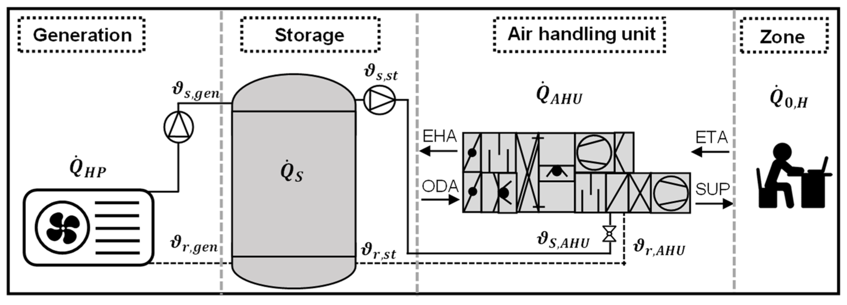
4.1. System Overview

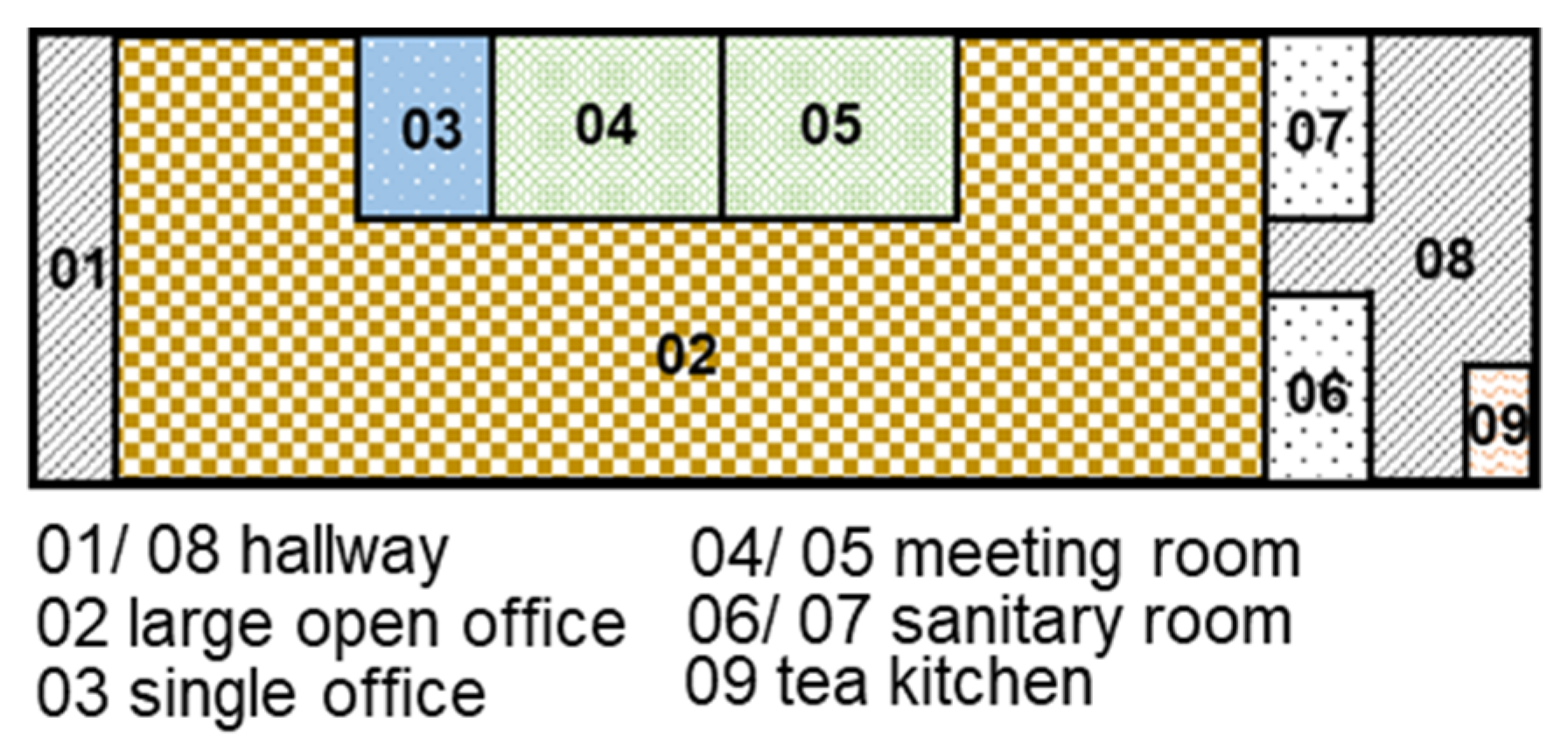
The BES consists of a heat pump, thermal storage tank, air conditioning system, and the building model (Figure 2). The model was created using TRNSYS [39], and its development is explained in the following sections.

4.2. Building Model

The building model represents an office. In addition to the individual and group offices, the model contains meeting rooms, sanitary rooms, and traffic areas and has a total area of 569 m² (Figure 3). The building insulation meets the requirements of the German Standard EnEV 2016 [40]. User behavior, internal heat emissions caused by people and devices, moisture, and pollutant emissions are defined in accordance with DIN EN 16798 [41]. The set heating temperature was assumed to be 20 °C in zones where occupants are frequently present (i.e., offices and meeting rooms), and a lower temperature standard (16 °C) was set in zones with occasional occupancy (i.e., hallways). The lower temperature standard also applied to time outside of open hours and on weekends. On weekends, no optimal ADR operation schedule was considered. The climatic boundary conditions correspond to the location of Stuttgart, Germany, which are represented by data from the German Weather Service. Under these conditions, the nominal heating load of the building is ${\dot{\mathrm{Q}}}_{0,\mathrm{H}}$ = 34 kW, according to DIN EN 12831 [42].

4.3. Air Handling Unit Model

The studied air conditioning system was a decentralized air-handling unit (AHU) that uses a PI controller to control the supply air temperature and airflow rate in each individual zone. During heating, recirculated air is used since it is more energetically efficient in terms of covering the thermal loads. The efficiency of the heat recovery was assumed as 80% and the system could be controlled by a bypass for frost protection. The outdoor air fraction was controlled based on the CO₂ concentration, with a limit of 600 ppm above the outside concentration [41]. The temperature difference in the heating coil in the nominal case was $\Delta \vartheta =$ 20 K, with the HVAC system having a supply temperature of ${\vartheta }_{\mathrm{s},\mathrm{st}}=$ 60 °C and a return temperature of ${\vartheta }_{\mathrm{r},\mathrm{st}}=$ 40 °C. To create the initial charging schedule, it was assumed that the temperature spread $\Delta \mathsf{\theta }$ drops from 20 °C to 5 °C as the supply temperature decreases from 60 °C to 40 °C. Each AHU has a nominal air volume flow rate of 400 m³/h, and the number of units in each zone depends on the floor area as well as on the nominal heating load.

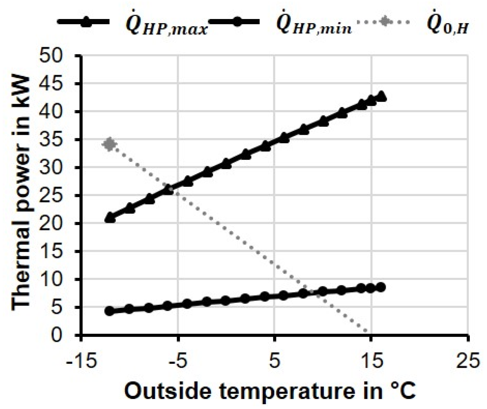
4.4. Heat Pump Model

The air-to-water heat pump system was designed in bivalent operation using an auxiliary heating unit with an efficiency of ${\mathsf{\eta }}_{\mathrm{H}}$ = 0.9. The minimal heating power and maximal heating power limit the working range of the heat pump, with the bivalence point at around −5 °C (Figure 4).

The supply temperature of the heat generator ${\vartheta }_{\mathrm{s},\mathrm{gen}}$ corresponds to the design temperature of the heating coil and is controlled depending on the ambient temperature. If the outdoor temperature is extremely cold (${\vartheta }_{\mathrm{Au}}\le$ −12 °C), the supply temperature is set to ${\vartheta }_{\mathrm{s},\mathrm{gen}}=$ 60 °C. For the upper temperature limit ${\vartheta }_{\mathrm{Au}}=$ 18 °C, the supply temperature is reduced accordingly to ${\vartheta }_{\mathrm{s},\mathrm{gen}}$ = 40 °C. Linear interpolation is assumed within these temperature limits. The COP depends on the dynamic operation point and, according to Bettanini et al. [43], can be idealized as a product of three terms (24): the full load efficiency ${\mathrm{COP}}_{\mathrm{fl}}$, the partial load factor (PLF), which takes into account the influence of thermal load, and the degradation coefficient due to the defrost factor (DOF).

$$\mathrm{COP}={\mathrm{COP}}_{\mathrm{fl}}·\mathrm{PLF}·\mathrm{DOF}$$

(24)

The functions of the three factors can be determined using the test data of the German standard DIN V 18599-5 [44]. More details can be found in Appendix A and Appendix B.

4.5. Storage Tank and Hydraulic System Model

The stratified storage tank model is shown with the corresponding temperature layers and mass flows in Figure 5, as are the positions of the inlet and outlet ports. The model represents a cylindrical storage tank and its volume is set with a height of 2 m (Volume 4.5 m³), which is equally divided into N = 20 temperature layers. The TES was modelled using TRNSYS component Type 158 [39], which solves differential Equation (15).

The left side of the tank indicates the connections to the heat pump, which can be charged by the inlet port (upper layer) with the corresponding supply temperature ${\vartheta }_{\mathrm{s},\mathrm{gen}}$ and the mass flow ${\dot{\mathrm{m}}}_{\mathrm{s},\mathrm{gen}}$ of the heat pump. The outlet port, which is located at the bottom layer of the left tank side, represents the return flow to the heat pump. Similarly, on the right side of the tank, the water with the corresponding supply temperature ${\vartheta }_{\mathrm{s},\mathrm{st}}$ and mass flow ${\dot{\mathrm{m}}}_{\mathrm{s},\mathrm{st}}$ is supplied to the AHU via the outlet port on the upper right side in case of heating demands in the building (discharging). The return flow from the AHU is connected to the lowest layer of the tank. It is assumed that the mass flows on both sides are identical when charging or discharging at the inlet and outlet port (${\dot{\mathrm{m}}}_{\mathrm{s},\mathrm{gen}}={\dot{\mathrm{m}}}_{\mathrm{r},\mathrm{gen}}$; ${\dot{\mathrm{m}}}_{\mathrm{s},\mathrm{st}}={\dot{\mathrm{m}}}_{\mathrm{r},\mathrm{st}})$. The supply temperature to the AHU is equal to the temperature of the upper layer, and the return temperature to the heat pump corresponds to the temperature of the bottom layer (${\vartheta }_{\mathrm{s},\mathrm{st}}={\vartheta }_1; {\vartheta }_{\mathrm{r},\mathrm{gen}}={\vartheta }_{20})$. When the design temperature of the air conditioning system to estimate the storage capacity are ${\vartheta }_{\mathrm{st},\min }=$ 40 °C in the bottom and ${\vartheta }_{\mathrm{st},\max }=$ 60 °C in the top layer, the energy capacity is 104 kWh [8]. The heat losses of the storage tank are calculated with an average heat transfer coefficient of 0.4 W/(m²∙K), and the ambient temperature of the TES is assumed to be 20 °C throughout the entire heating period. The initial water temperature at the beginning of the year (simulation start) was set to 40 °C. The heat loss in the pipeline to the ambient areas is neglected [30]. Based on the nominal temperature difference $\Delta {\mathsf{\theta }}_{\mathrm{des}}$ and heating load ${\dot{\mathrm{Q}}}_{0,\mathrm{H}}$, the design mass flow rate of the hydraulic system is given by (25).

$${\dot{\mathrm{m}}}_{\mathrm{des}}=\frac{{\dot{\mathrm{Q}}}_{0,\mathrm{H}}}{{\mathrm{c}}_{\mathrm{p},\mathrm{w}}·\Delta {\mathsf{\theta }}_{\mathrm{des}}}$$

(25)

The auxiliary power of the hydraulic pump ${\mathrm{P}}_{\mathrm{el},\mathrm{P}}$ is determined by the flow rate ${\dot{\mathrm{V}}}_{\mathrm{total}}$, the pressure losses $\Delta {\mathrm{p}}_{\mathrm{HV}}$, and the efficiency of the pump ${\mathsf{\eta }}_{\mathrm{P}}$ according to (26).

$${\mathrm{P}}_{\mathrm{el},\mathrm{P}}=\frac{{\dot{\mathrm{V}}}_{\mathrm{total}}·\Delta {\mathrm{p}}_{\mathrm{HV}}}{{\mathsf{\eta }}_{\mathrm{P}}}$$

(26)

4.6. Pre-Processing of Model Inputs

4.6.1. Grid-Supportive Signal

Time-variable grid-supportive signals are based on the price of electricity (24 h day-ahead price) [45] and the carbon dioxide emissions (CDE) of electricity generation in Germany. The level of direct emissions depends on the type of electricity source participating in electricity generation at each specific time. The data are available 24 h ahead for each upcoming day [46]. Only direct emissions are observed; thus, potential indirect emission reductions in electricity generation, e.g., by emission certificates, are not considered. Furthermore, the effects on the energy market are not reflected when the signal is used for ADR control purposes [47]. The carbon dioxide equivalents conducted are listed in Appendix A. For the definition of low, medium, and high electricity grid utilization, the grid-supportive signal g(t) is categorized into three discrete signals by determining the range for each day (27).

$$\Delta \mathrm{S}={\mathrm{g}}_{\max }(\mathrm{t})-{\mathrm{g}}_{\min }(\mathrm{t})$$

(27)

Accordingly, the time periods with the corresponding signals are classified into the three levels (I, II, and III). Low-level grid signals (G(t) = I) correspond to time durations with an electricity surplus in the grid or when there is a large share of electricity from renewable energy sources—the generation exceeds the demand. On the contrary, high-level grid signal levels (G(t) = III) represent the peak hours when electricity generation is relatively low compared to the demand. Figure 6 illustrates the grid signal classification using an exemplary day from 2017.

It is obvious that there can be significant fluctuations during the day, with the price signal generally indicating a comparatively lower price at night and higher electricity prices in the morning and early evening. The CDE grid signal pattern shows similar characteristics, although the minimum usually occurs in the afternoon due to the fluctuating amounts of renewable electricity that are generated. The variation in the CDE is not as significant compared to the price signal and tends to vary with the seasons. Changes may occur due to climatic influences and between workdays and weekends.

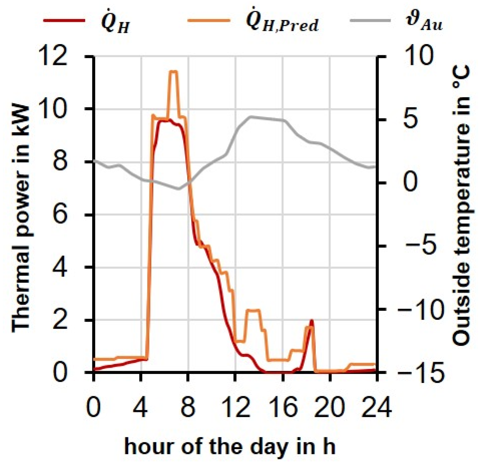
4.6.2. Load Prediction Model

In the case of a data-driven model, different machine learning methods are suitable for predicting the daily heating energy demand of buildings. Among the classical regression methods, the support vector method, Gaussian process regression, and regression trees are appropriate models [48,49]. In this case study, a regression tree (RT) model is used. Using RT as a data-based model, the input data is processed iteratively and recursively, aiming to define the most possible class assignment for a specified property of the different parameters [50]. For this purpose, the input data is divided into groups in the form of a tree, consisting of a root node, several branch nodes, and the bottom level (output). Each information content (28) is weighted and processed by the probability of its occurrence (information entropy),

$$\mathrm{E}(\mathrm{S})={\displaystyle \sum }_{\mathrm{i}=1}^{\mathrm{n}}-{\mathrm{p}}_{\mathrm{i}}·{\log }_2({\mathrm{p}}_{\mathrm{i}})$$

(28)

where n represents the number of different target values and p_i is the probability of each data group. The so-called Iterative Dichotomiser 3 algorithm (ID3) [51] was used to generate the RT. The prediction approach for data-driven modelling can be divided into the three common steps according to supervised learning [52]: data preparation, data processing (model training), and prediction. The number of input data during data preparation (training variables) and the training data affect the prediction accuracy. Suitable training variable selection is usually carried out by testing and checking and is always a compromise between the prediction accuracy versus the challenge of specifying certain parameters. In this study, only very commonly measurable and accessible smart building parameters are considered as training variables (

Table 1. Training parameters of the load prediction model.

Parameter	Range of Values	Unit
Weekday	Mo…Fr	-
Hour of the day	0…24	h
Presence of users	0…1	-
Set temperature	16…20	°C
Outdoor temperature	−12…35	°C
Solar radiation	0…928	W/m2
Daily heat load	0…28	kW

).

The simulation results for the BES (heating period) that were described in Chapter 3 were used as training data using the Test Reference Year (TRY) [53] of Stuttgart as weather data. For prediction purposes as well as for the simulations using the MPC strategy, historical data from 2017 [54] are obtained and provided as weather forecasts. An exemplary prediction of the daily heating power load ${\dot{\mathrm{Q}}}_{\mathrm{H},\mathrm{Pred}}$ compared to the real thermal load ${\dot{\mathrm{Q}}}_{\mathrm{H}}$ of the BES simulation is shown in Figure 7.

The comparison between the forecast and the real heating power for the exemplary winter day shows good agreement with R² = 0.97 and the RMSE = 0.78 kW. During the year, however, there are days with significantly lower prediction accuracy. The accuracy for the entire heating period (2017) is R² = 0.71 and RMSE = 1.53 kW.

4.6.3. Signal for the Heating Requirement

If the outdoor temperature ${\vartheta }_{\mathrm{Au}}$ is below 18 °C during the building’s office hours (8 a.m.−19 p.m.), then it is assumed that there is a heating requirement for this day (H_t = 1). Otherwise, H_t is set to H_t = 0 and the heating system stays off during the day. Signal H is determined at the beginning of each day based on the weather forecast.

4.7. MPC Implementation

As a bivalent heat pump coupled with TES is considered in the heating system, the object function (20) can be instantiated into (29), which aims to minimize the electricity consumption of the heating system based on the grid-supportive signal. The electricity power is the sum of the power of the heat pump ${\mathrm{P}}_{\mathrm{el},\mathrm{gen}}$ and the circulation pump ${\mathrm{P}}_{\mathrm{p}}(\mathrm{t})$. Two different grid-supportive signals, the day-ahead electricity price ${\mathrm{C}}_{\mathrm{el}}$ and the carbon dioxide emission rate CDE_el, will be discussed. The boundary conditions of the MPC strategy are represented by (30)–(34). Since electricity is pure usable energy, the boundary conditions remain unchanged and the objective function (29), as well as the boundary constraints (30)–(34), are identical for both exergy-based and energy-based control strategies. In (30) to (32), the bivalent operation of the heat pump is considered. ${\dot{\mathrm{Q}}}_{\mathrm{gen}}$ represents the thermal power provided by the heat generator, which consists of the thermal power of the heat pump ${\dot{\mathrm{Q}}}_{\mathrm{HP}},$ and the electrical heating tab ${\dot{\mathrm{Q}}}_{\mathrm{HT}}$. ${\dot{\mathrm{Q}}}_{\mathrm{HP},\max }$ specifies the upper and lower limit ${\dot{\mathrm{Q}}}_{\mathrm{HP},\min }$ of the thermal power provided by the heat generator (31). The electrical power of the heat generator is calculated by considering the variable COP of the heat pump (Section 4.4) and a constant efficiency of the heating tab ${\mathsf{\eta }}_{\mathrm{H}}=$ 0.9 (32). The initial charging schedule indicates that the heat generator charges the storage tank with nominal power (33). Moreover, (34) was used to calculate the electrical power of the circulation pump. Since a simplified hydraulic system is adopted in this study, the circulation pump power is correlated with the predicted heat load ${\dot{\mathrm{Q}}}_{\mathrm{H},\mathrm{Pred}}$. When implementing exergy or energy analysis in the MPC strategy, it is important to note that a fluid with the same energy quantity can provide a different exergy quantity. Therefore, the XMPC strategy uses (35), which describes the required transient exergy stored in the TES for flexible operation throughout the entire day. On the contrary, in the EMPC strategy, (36) is applied to guarantee that the heating demands for the HVAC system can be covered during the day.

$$\min \mathrm{J}={\displaystyle \sum }_{\begin{array}{c}\mathrm{t}=1\\ \mathsf{\tau }=\mathrm{1}\mathrm{h}\end{array}}^{24}({\mathrm{P}}_{\mathrm{el},\mathrm{gen}}(\mathrm{t})·\overrightarrow{\mathrm{X}}(\mathrm{t})·\mathrm{g}(\mathrm{t})·\mathsf{\tau }+{\mathrm{P}}_{\mathrm{el},\mathrm{p}}(\mathrm{t})·\mathrm{g}(\mathrm{t})·\mathsf{\tau }))$$

(29)

s.t.

$${\dot{\mathrm{Q}}}_{\mathrm{gen}}(\mathrm{t})={\dot{\mathrm{Q}}}_{\mathrm{HP}}(\mathrm{t})+{\dot{\mathrm{Q}}}_{\mathrm{HS}}(\mathrm{t})$$

(30)

$${\dot{\mathrm{Q}}}_{\mathrm{HP},\min }(\mathrm{t})\le {\dot{\mathrm{Q}}}_{\mathrm{HP}}(\mathrm{t})\le {\dot{\mathrm{Q}}}_{\mathrm{HP},\max }(\mathrm{t})$$

(31)

$${\mathrm{P}}_{\mathrm{el},\mathrm{gen}}(\mathrm{t})=(\frac{{\dot{\mathrm{Q}}}_{\mathrm{HP}}(\mathrm{t})}{\mathrm{COP}}+\frac{{\dot{\mathrm{Q}}}_{\mathrm{HT}}(\mathrm{t})}{{\mathsf{\eta }}_{\mathrm{H}}})$$

(32)

$$\overrightarrow{\mathrm{X}}(\mathrm{t})\in \left\{0,1\right\}$$

(33)

$${\mathrm{P}}_{\mathrm{el},\mathrm{p}}(\mathrm{t})=\mathrm{f}({\dot{\mathrm{Q}}}_{\mathrm{H},\mathrm{Pred}})$$

(34)

$$-{\displaystyle \sum }_{\mathrm{k}=1}^{\mathrm{k}=\mathrm{t}}{(1-\mathrm{SF})}^{\mathrm{t}-\mathrm{k}}·{\dot{\mathsf{\Xi }}}_{\mathrm{gen}}(\mathrm{t})·\overrightarrow{\mathrm{X}}(\mathrm{t})·\mathsf{\tau }\le {\mathsf{\Xi }}_{\mathrm{st},0}·{(1-\mathrm{SF})}^{\mathrm{t}}-{\displaystyle \sum }_{\mathrm{k}=1}^{\mathrm{k}=\mathrm{t}}{(1-\mathrm{SF})}^{\mathrm{t}-\mathrm{k}}·{\dot{\mathsf{\Xi }}}_{\mathrm{H}}(\mathrm{t})·\mathsf{\tau }$$

(35)

or:

$$-{\displaystyle \sum }_{\mathrm{k}=1}^{\mathrm{k}=\mathrm{t}}{(1-\mathrm{SF})}^{\mathrm{t}-\mathrm{k}}·{\dot{\mathrm{Q}}}_{\mathrm{gen}}(\mathrm{t})·\overrightarrow{\mathrm{X}}(\mathrm{t})·\mathsf{\tau }\le {\mathrm{E}}_{\mathrm{st},0}·{(1-\mathrm{SF})}^{\mathrm{t}}-{\displaystyle \sum }_{\mathrm{k}=1}^{\mathrm{k}=\mathrm{t}}{(1-\mathrm{SF})}^{\mathrm{t}-\mathrm{k}}·{\dot{\mathrm{Q}}}_{\mathrm{H},\mathrm{Pred}}(\mathrm{t})·\mathsf{\tau }$$

(36)

Taking energy or exergy losses, irreversibility, and deviations in the load prediction into consideration, a safety factor SF was used. As there are not many SF reference values for XMPC, the value of 0.5% per hour (12% per day), which was recommended in previous EMPC research [30], was initially adopted in this study. Three assumptions were made to provide an estimation of the temperatures and to make the exergy predictions for XMPC, thereby allowing (35) to be solved. First, it was assumed that the supply temperature ${\vartheta }_{\mathrm{s},\mathrm{gen}}$ and the return temperature ${\vartheta }_{\mathrm{r},\mathrm{gen}}$ of the heat generator were equal to the temperature at the top and bottom of the storage tank. Second, it was assumed that the storage tank had a linear stratification. The temperature of the water supply for the HVAC system ${\vartheta }_{\mathrm{s},\mathrm{st}}$ was equal to the temperature of the first layer of water in the tank; however, depending on the discretization accuracy, it could be lower than the heat pump supply temperature ${\vartheta }_{\mathrm{s},\mathrm{gen}}$. In this case, it was assumed that the tank had a 5% temperature spread (${\vartheta }_{\mathrm{s},\mathrm{gen}}-{\vartheta }_{\mathrm{r},\mathrm{gen}}$) for the temperature difference since the entire tank was discretized into 20 layers. Third, a linear correlation between the temperature spread $\Delta \mathsf{\theta }$ and the supply temperature ${\vartheta }_{\mathrm{s},\mathrm{st}}$ was assumed in order to approximate the behavior of the heating system as a function of the ambient conditions (details in Section 4.3). With these assumptions, the predicted exergy demand ${\dot{\mathsf{\Xi }}}_{\mathrm{H}}$ and exergy supply capability of the heat generator ${\dot{\mathsf{\Xi }}}_{\mathrm{gen}}$ (Section 3.2) could be computed and used to create the initial charging plan $\overrightarrow{\mathrm{X}}$. It can be seen that both the objective function and the boundary conditions are linear functions of $\overrightarrow{\mathrm{X}}(\mathrm{t})$. Since $\overrightarrow{\mathrm{X}}(\mathrm{t})$ is a binary integer vector, the optimal scheduling problem can be solved using a mixed integer linear programming (MILP) algorithm. In this paper, the MATLAB optimization toolbox [55] was chosen because of its fast computation and good compatibility with TRNSYS. After the initial charging schedule was computed, the control strategy proceeded to the second phase during the simulation and performed the rule-based calibration described in Section 3.3. The time resolution of the calibration was 5 min.

5. Results and Evaluation of the Control Strategy

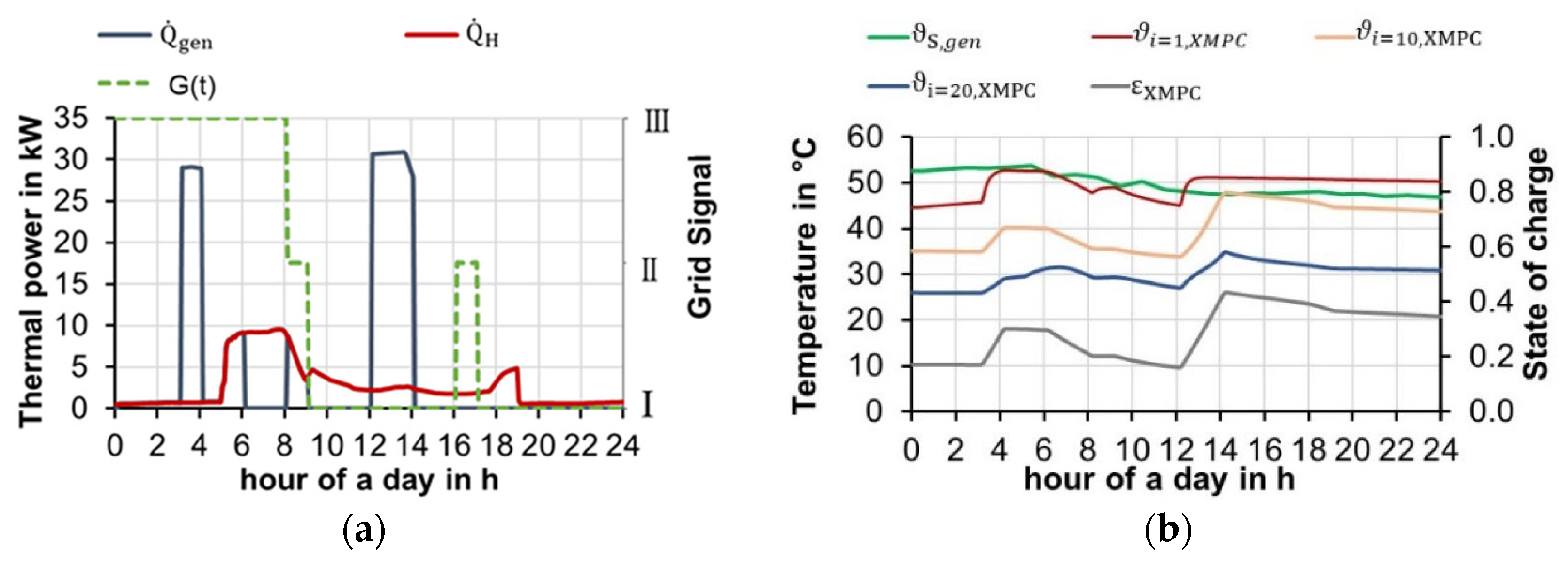
5.1. Analysis on Characteristic Days

The results of the simulations with EMPC and XMPC are analyzed for individual characteristic days (

Table 2. Typical days for the location of Stuttgart, Germany (2017).

Typical Day	Temperature	Appearance Frequency
Cold day	−15 °C to −5 °C	10 days
Cool day	−5 °C to 5 °C	88 days
Moderate day	5 °C to 15 °C	162 days

), which represent typical loads for the heating period in Stuttgart.

To prospectively illustrate the amount of stored exergy within the TES during ADR operation, the state of charge $\mathsf{\epsilon }$ is introduced. According to (37), $\mathsf{\epsilon }$ is defined as the ratio of the stored exergy or energy to the maximum storage capacity (Section 4.5).

$$\mathsf{\epsilon }(\mathrm{t})=\frac{{\mathsf{\Xi }}_{\mathrm{st}}(\mathrm{t})}{{\mathsf{\Xi }}_{\mathrm{st},\max }} \mathrm{or} \mathsf{\epsilon }(\mathrm{t})=\frac{{\mathrm{E}}_{\mathrm{st}}(\mathrm{t})}{{\mathrm{E}}_{\mathrm{st},\max }}$$

(37)

Figure 8, Figure 9 and Figure 10 present daily analyses of typical days for both the energy (EMPC) and exergy (XMPC) models during ADR operation. More specifically, the load curves on the left axis of the left illustration represent the thermal power of the heat pump (blue lines) and the heating load of the AHU (red line). On the secondary axis, the discrete grid control signal G(t) is shown (green line). The results are carried out with the day-ahead price as the grid-supportive signal. The variant with the CDE factor as a grid-supportive signal is discussed separately in Section 5.3.1. In each graph on the right-hand side, the thermal stratification within the tank and the supply temperature of the heat pump ${\vartheta }_{\mathrm{s},\mathrm{gen}}$ are illustrated on the left-axis, while the state of the charge is presented on the secondary axis. The thermal stratification within the TES is demonstrated by the fluid temperature of the layers at the bottom ${\vartheta }_{\mathrm{i}=20}$, in the middle ${\vartheta }_{\mathrm{i}=10}$, and at the top ${\vartheta }_{\mathrm{i}=1}$.

On a typical cold day, the main EMPC and XMPC charging durations extend throughout the entire night—from 0:00 to the early morning at 6:00. This day is among those with the highest energy requirements, which is seen during the heat load-oriented charging hours after 6:00, when the discrete control signal changes to the middle-level. For EMPC, the overall high temperature level leads to a gradual decrease in the heat flux supplied by the heat generator after 4:00, since the return temperature to the heat generator increases significantly as the state of charge increases. Over the course of the day, especially when the grid signal is at a high level, the heat pump remains off and the storage tank is discharged to a large extent. In order to provide sufficient energy quantity within the tank, the heat generator is temporarily in heat load-oriented operation between 12:00 and 16:00 and is charged for some time with EMPC at a nominal power level. Although the temperature level and the state of charge of the previous day are slightly higher when using EMPC compared to XMPC, the generator runs in demand-based operation with EMPC for about one hour after the main charging period (00:00 to 6:00). The temperature difference in the thermocline during daily operation with XMPC is about 17 K to 35 K, while the minimum temperature difference due to stratification with EMPC is just 10 K (around 5:00 am). On this cold day, besides the minor variations in the charging cycle, the differences of the temperature distribution within the tank are most important. It can be seen that the temperature level for EMPC and thus the stored energy is higher compared to XMPC.

On a cool day (Figure 9), the heat generator with the XMPC runs at nominal power from 0 to 5 o’clock to optimally utilize the interval with a low-level grid signal and stays off during the high-level grid signals.

Under the same conditions, the EMPC strategy continues to charge the TES in heat load-oriented mode until around 7 o’clock when the grid signal reaches the middle-level, although the initial temperature level is slightly higher compared to that on a cold day. Moderate days have a comparatively low heating energy demand, so the storage tank does not require charging on all of these days. Figure 10 shows a moderate day with a brief charging duration in the early morning (4:00) using both methods. EMPC had already performed a brief charging procedure at 1:00. Stratification with the XMPC maintains a range of 10–20 K, while the water temperatures of the different layers with EMPC reach almost the same level at 5:00.

The typical daily analyses demonstrate that exergy-based control provides a higher capability to maintain appropriate stratification than the EMPC under the same boundary conditions. Additionally, the XMPC charging durations are able to adapt to momentary grid utilization more quickly compared to EMPC, increasing its ability to exploit the flexibility potential based on the variable grid-supportive signal. This is further validated by the annual results discussed in the following section.

5.2. Analysis of Annual Simulation

The annual simulation results of the XMPC and EMPC strategy are compared with the Reference Model, where the heat generator supplies the AHU system directly without the operation of either TES or ADR. Correspondingly, the heat generator runs in the Reference Model in the heat load-oriented mode all the time.

5.2.1. Dynamic Exergy and Energy Analysis

The exergy quantities according to the balance Equation (7) as well as the overall exergy efficiency are listed in

Table 3. Annual EMPC exergy analysis.

Month	${\mathsf{\Xi }}_{\mathbf{i}\mathbf{n}}$	${\mathsf{\Xi }}_{\mathbf{r}\mathbf{e}\mathbf{c}}$	${\mathsf{\Xi }}_{\mathbf{l}\mathbf{o}\mathbf{s}\mathbf{s}}$	${\mathsf{\Xi }}_{\mathbf{d}\mathbf{e}\mathbf{s}}$	$\mathbf{\Delta }\mathsf{\Xi }$	$\mathsf{\psi }$
	(kWh)	(kWh)	(kWh)	(kWh)	(kWh)	(%)
Jan	311.6	272.3	10.7	30.0	−1.4	87.4
Feb	80.0	56.7	8.1	10.7	4.5	70.9
Mar	15.2	4.8	9.6	1.7	−0.9	31.4
Apr	11.3	0.0	11.0	0.2	0.1	0.4
May	7.0	0.0	9.1	0.1	−2.3	0.0
Jun	7.2	0.0	6.5	0.1	0.6	0.0
Jul	5.3	0.0	6.3	0.1	−1.0	0.0
Aug	6.8	0.0	6.1	0.1	0.6	0.0
Sep	9.8	0.0	8.8	0.1	0.8	0.0
Oct	13.1	0.0	9.3	0.1	3.6	0.3
Nov	80.3	64.6	8.7	10.9	−4.0	80.5
Dec	157.4	128.8	8.2	73.8	1.4	81.8
Sum	704.9	527.2	102.5	127.9	2.0	74.8

and

Table 4. Annual XMPC exergy analysis.

Month	${\mathsf{\Xi }}_{\mathbf{i}\mathbf{n}}$	${\mathsf{\Xi }}_{\mathbf{r}\mathbf{e}\mathbf{c}}$	${\mathsf{\Xi }}_{\mathbf{l}\mathbf{o}\mathbf{s}\mathbf{s}}$	${\mathsf{\Xi }}_{\mathbf{d}\mathbf{e}\mathbf{s}}$	$\mathbf{\Delta }\mathsf{\Xi }$	$\mathsf{\psi }$
	(kWh)	(kWh)	(kWh)	(kWh)	(kWh)	(%)
Jan	276.6	245.7	7.2	25.5	−1.9	88.9
Feb	67.4	52.8	5.8	6.1	2.7	78.4
Mar	9.3	4.3	5.8	1.0	−1.8	45.7
Apr	7.5	0.0	6.3	0.4	0.9	0.5
May	1.6	0.0	3.7	0.2	−2.2	0.1
Jun	3.6	0.0	2.4	0.4	0.8	0.0
Jul	3.0	0.0	2.7	0.3	0.0	0.0
Aug	3.3	0.0	3.3	0.2	−0.2	0.0
Sep	4.9	0.0	4.0	0.3	0.5	0.0
Oct	10.1	0.0	4.7	0.4	5.0	0.3
Nov	70.7	61.4	6.8	6.7	−4.2	86.8
Dec	147.0	125.7	6.5	55.5	0.2	85.5
Sum	605.0	490.0	59.3	96.9	−0.3	81.0

. It can be seen that with both approaches, more declines in the exergy are caused by destruction ${\mathsf{\Xi }}_{\mathrm{des}}$ (i.e., irreversibility) rather than exergy loss ${\mathsf{\Xi }}_{\mathrm{loss}}$ during an annual cycle. As shown in the tables, especially during colder periods (i.e., Dec. to Jan.), exergy destruction dominates, while in moderate months (i.e., Mar. to Oct.) the decrease in the available exergy is mainly due to exergy losses. As for the overall exergy efficiency $\mathsf{\psi }$, both of the control strategies showed the same tendency—higher in cold months and lower in mild months. Comparing the absolute values of EMPC and XMPC, it is obvious that the XMPC strategy has a significantly higher exergy efficiency, especially in the moderate months. Thus, the total annual exergy efficiency is about 6% higher with the XMPC. The exergy that is consumed by the HVAC system ${\mathsf{\Xi }}_{\mathrm{rec}}$ of both models is comparable, although the exergy that is provided by the heat generator is considerably higher with the EMPC. The differences in the exergy that is delivered is mainly due to the state of charge at a certain time, which may vary due to different charging cycles. Thus, the supply temperature as well as the return temperature of the HVAC system may also differ during real-time operation. Nevertheless, it can be shown that XMPC is able to recover more exergy for the heating supply and that it can provide greater amounts of usable energy to the HVAC system. With the XMPC strategy, the annual exergy loss drops by about 42%, from 102.5 kWh to 59.3 kWh, which again proves that XMPC allows for more appropriate stratification within the TES to be maintained and that allows for better adaptation to actual HVAC demand.

More adequate stratification reduces unnecessary heat losses, especially during the moderate months. The exergy analysis demonstrates that the XMPC strategy is more flexible and effective during ADR operation compared to EMPC.

5.2.2. Load Shifting Potential and Electricity Utilization

The shifted energy can be evaluated according to (38) via the predefined time durations of the low (G(t) = I), middle (G(t) = II), and high (G(t) = III) electricity grid utilization levels.

$${\mathrm{W}}_{\mathrm{el}}=\underset{\mathrm{G}(\mathrm{t})=\mathrm{I}}{\overset{}{{\displaystyle \int }}}{\mathrm{P}}_{\mathrm{el}}\mathrm{dt}+\underset{\mathrm{G}(\mathrm{t})=\mathrm{II}}{\overset{}{{\displaystyle \int }}}{\mathrm{P}}_{\mathrm{el}}\mathrm{dt}+\underset{\mathrm{G}(\mathrm{t})=\mathrm{III}}{\overset{}{{\displaystyle \int }}}{\mathrm{P}}_{\mathrm{el}}\mathrm{dt}$$

(38)

Figure 11 shows the electricity demand of the Reference Model, as well as during ADR operation, and is categorized according to the grid utilization level. It can be seen that in the case of the Reference Model, electricity utilization often occurs (34%) during peak hours, when the price is highest (G(t) = III), while over 28% of the electricity utilization occurs at the middle price level (G(t) = II), and 37% of the total demand occurs at the low-price level. Considering ADR operation, most of the electricity utilization—more than 80% with EMPC and over 83% with XMPC, respectively—occurs during low-price times (G(t) = I). Only a minor part of the electricity utilization takes place when higher price levels are in effect (G(t) = III).

It can be seen that during ADR operation, the total annual electricity demand declines compared to the Reference Model, decreasing from 10.2 to 9.3 kWh/(m²∙a) for the EMPC and, most significantly, for the XMPC—with an overall reduction from 27% to 7.4 kWh/(m²∙a). The reduction in the total electricity demand during ADR operation is due to the higher overall efficiency of the heat generator, which is further discussed in the next section.

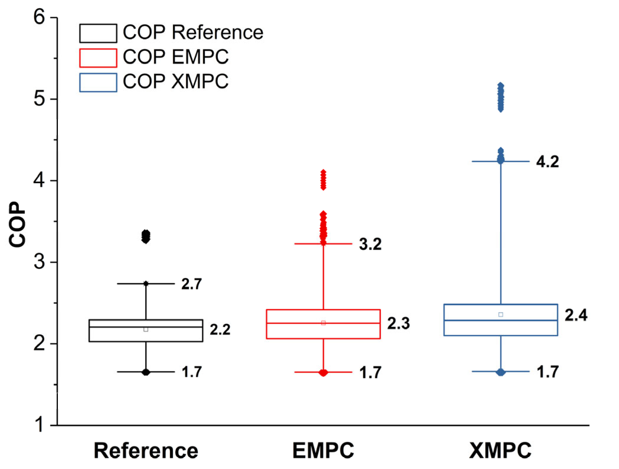
5.2.3. Efficiency of the Heating Generator

The coefficient of performance (COP) as well as the seasonal coefficient of performance (SCOP) of the heat pump in the annual cycle are analyzed according to (39) and (40).

$$\mathrm{COP}=\frac{{\dot{\mathrm{Q}}}_{\mathrm{HP}}}{{\mathrm{P}}_{\mathrm{el},\mathrm{HP}}}$$

(39)

$$\mathrm{SCOP}=\frac{{\mathrm{Q}}_{\mathrm{HP}}+{\mathrm{Q}}_{\mathrm{HT}}}{{\mathrm{W}}_{\mathrm{el},\mathrm{gen}}}=\frac{{\mathrm{Q}}_{\mathrm{HP}}+{\mathrm{Q}}_{\mathrm{HT}}}{{\mathrm{W}}_{\mathrm{el},\mathrm{HP}}+\frac{{\mathrm{Q}}_{\mathrm{HT}}}{{\mathsf{\eta }}_{\mathrm{H}}}}$$

(40)

The MPC strategies during ADR operation with TES allow for higher COP and SCOP values, which explains the total reduction in electric energy despite the increased demand for thermal energy. The annual COP distribution throughout the entire heating period can be found in Appendix C. As shown in Figure 12a, SCOP is increased by 28% with EMPC and by 53% with XMPC during ADR operation compared to the Reference Model. The results support the conclusions of other researchers, which indicate that by using TES in combination with an appropriate control strategy, the efficiency of the heat generator in a building energy system can be increased [10,56]. Apart from COP, the XMPC method defines a more appropriate operating time for the heat pump in order to minimize the auxiliary electrical heating power, as observed in Figure 12b. The thermal energy that is generated by auxiliary electrical heating accounts for about 40% compared to the Reference Model, while it is reduced to 18% with EMPC and to 6% with XMPC. It can also be seen from Figure 12b that the ADR operation with the TES slightly increases the thermal energy demand of the heat generator compared to the Reference Model—by 16% with EMPC and 11% with XMPC. This is mainly due to the losses related to irreversibility and heat transfer to the ambient area. It has also been concluded by other researchers that TES deployment can increase the total energy demand of a building’s energy system [56].

Ideally, the TES should be capable of providing the thermal power required by the HVAC system at any time. To evaluate the heating supply, the time durations are accumulated as a percentage of the dissatisfied hours (PDH) when the thermal power supplied from the TES during ADR operation is insufficient, i.e., lower than the heat load of the building (${\dot{\mathrm{Q}}}_{\mathrm{rec}}(\mathrm{t})<{\dot{\mathrm{Q}}}_{\mathrm{H}}(\mathrm{t})$). In addition, the insufficiently supplied energy is summed up as being deficit energy throughout the entire year. For both the EMPC and XMPC strategy, the PDH is less than 0.2%, while the insufficient delivered energy for each model is 0.6%. In order to achieve the same performance, the safety factor must be increased to 5% with EMPC. Once again, this indicates that the exergy-based methodology has a higher capability of providing the required thermal energy for the HVAC system.

5.2.4. Operating Costs and Carbon-Dioxide Emissions

The operating costs (OC) and the CDE were calculated using (41) and (42), respectively [24,30,57].

$$\mathrm{OC}={\displaystyle \sum }_{\mathrm{t}=1}^{\mathrm{n}}{\mathrm{C}}_{\mathrm{el}}(\mathrm{t})·{\mathrm{W}}_{\mathrm{el}}(\mathrm{t})$$

(41)

$$\mathrm{CDE}={\displaystyle \sum }_{\mathrm{t}=1}^{\mathrm{n}}{\mathrm{CDE}}_{\mathrm{el}}(\mathrm{t})·{\mathrm{W}}_{\mathrm{el}}(\mathrm{t})$$

(42)

The results are illustrated and compared in Figure 13. Compared to the Reference Model, EMPC and XMPC achieve reductions in both OC and CDE. The EMPC strategy achieves a 34% reduction in the OC and a 10% decrease in the annual CDE. With XMPC, the annual OC drops to 0.27 EUR/(m²∙a) (47%), and CDE declines to 3.95 kgCO₂/(m²∙a) (27%)—a further 13% and 17% reduction in OC and CDE, respectively, compared to EMPC. Although MPC-based optimization aims to minimize costs, it achieved a reduction in the CDE as well. As more electricity is generated by renewable energy sources in the grid, electricity costs will be lower and less greenhouse gases will be emitted.

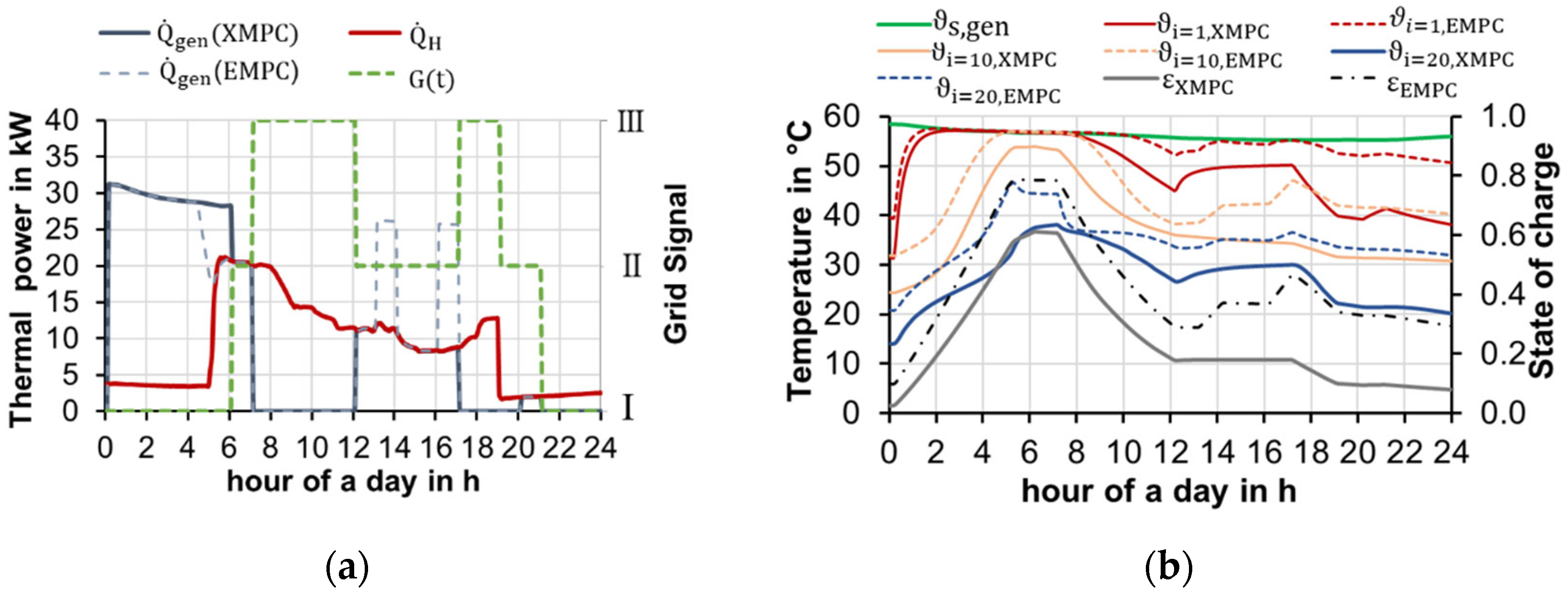
5.3. Stability and Sensitivity Analysis

In order to examine the stability of the proposed methodology, three key parameters—the grid-supportive signal, the size of the TES, and the heat pump—are studied further. A sensitivity analysis was carried out for the XMPC strategy since its overall performance is higher compared to the EMPC strategy.

5.3.1. Influence of the Grid-Supportive Signal

When considering the energy-related emissions as the grid-supportive signal, it is obvious that, in contrast to the electricity price, the time intervals in the early morning hours before occupancy tend to be less eligible for charging than the time intervals in the afternoon. The following analysis will demonstrate how the XMPC handles the different characteristics of the grid signal. All of the other inputs, the physical model in the TRNSYS, and the parameters of the control strategy in ADR operation remain unchanged, and the signal is processed in the same manner (Section 4.6.1). Compared to the results for a typical cool day shown in Section 5.1 along with the cost of the grid signal (Figure 9), the charging behavior during the day is quite different when using the CDE grid signal, as shown in Figure 14. The grid signal remains at a high level throughout the night (0:00–8:00). In order to provide enough energy during office hours, the heat generator charges the tank at nominal power from 3:00 to 4:00 and in the heat-oriented mode from 6:00 to 8:00, even when the grid signal is at a high level (G(t) = III). During the day, the heat generator runs at nominal power again from 12:00 to 14:00, when the grid indicates high availability (G(t) = I).

As shown in Figure 14b, the temperature increases during the charging durations and then drops as the storage tank is discharged. Compared to the Reference Model, the annual thermal energy demand increases by 10%, while the hours with insufficient thermal power and annual insufficient energy during operation are just 0.2% and 0.1%, respectively. The MPC strategy demonstrates good compatibility with different grid signal characteristics. Given that the CDE grid signal tends to be lower during the daytime—when the ambient temperature is relatively high—the heat pump is able to operate at a slightly higher COP and SCOP. Due to the improved efficiency of the heat generator and the slightly reduced thermal energy demand during ADR operation, the total annual electricity demand is reduced by 26%. With the CDE grid signal, XMPC achieves minimal annual emissions of 3.93 kg/(m²∙a)—another 6% reduction compared to the price of electricity for the grid signal. Figure 15 shows the flexibility potentials for different grid utilization levels by comparing the electricity price (XMPC-OC) and the CDE (XMPC-CDE) as grid-supportive signals, respectively. The simulation results were categorized into three variations based on the grid-supportive signal that was used in the control strategy (Reference, XMPC-CDE, XMPC-OC) and were evaluated according to the grid signal level (labels). The electric energy demand values are given in percentages. Regarding the CDE grid signal level (left column in each group), the high-level electricity demand (G(t)_CDE = III) is the most reduced when XMPC-CDE is implemented—by about 26%; similarly, the low-level electricity demand (G(t)_CDE = I) is greatly increased with XMPC-CDE—by about 21%. In terms of the day-ahead price grid signal, XMPC-OC achieves the maximum reduction in electricity demand at the high-level (G(t)_OC = III)—by about 42%—while XMPC-CDE only reached a decrease of about 16%. With respect to the changes in the operating costs and the CDE, both grid-supportive signals show a similar overall tendency, again indicating that the electricity price and CDE have a positive correlation with one another.

If the variability of the grid signal is considered its own during the control strategy by adjusting the optimization boundary conditions accordingly (32), the reductions can be determined without considering a heat pump. The electricity costs are thus reduced by 25%.

5.3.2. Influence of the Tank Size

The size of the TES could affect the performance of the entire energy system, especially in terms of ADR operation [15]. Considering the baseline model, two scenarios are examined, one with a 50% increase and another with a 50% decrease in volume. The results of the simulations are listed in

Table 5. Results of storage size variations.

Size	PDH	Insufficient Energy	${\mathbf{Q}}_{\mathbf{H}}$	${\mathbf{W}}_{\mathbf{e}\mathbf{l}}$	${\mathbf{C}}_{\mathbf{o}\mathbf{p}}$	CDE
(%)	(%)	(%)	(kWh/(m2∙a))	(kWh/(m2∙a))	(EUR/(m2∙a))	(kg/(m2∙a))
−50	0.3	0.78	15.22	8.35	0.336	4.42
0	0.2	0.61	15.55	7.43	0.274	3.95
50	0.3	0.55	16.08	7.46	0.271	3.98

. Both PDH and the insufficient delivered energy are comparable in these three variations. As the size of the TES increases, the annual thermal energy consumption increases slightly due to the higher heat losses to the ambient area. The electricity demand, which results from the heating demand and the SCOP of the heat pump (40), declines as the storage size increases. This is due to the higher SCOP of the heat generator when a larger tank size is deployed.

If the tank volume varies between −50% and +50%, then the annual operating costs decline by about 24% and the CDE declines by 11%. This is due to the higher storage capacity, which increases the shifted energy quantities during the ADR event. This is also reflected in the electricity utilization breakdown according to the grid signal level (

Table 6. Electrical energy demand according to grid signal (electricity price).

Tank Size	G(t) = I	G(t) = II	G(t) = III	Relative Electricity Utilization in %
−50%	72%	27%	3%	82
Baseline	84%	15%	1%	73
50%	86%	13%	1%	73

). If the size of the TES is decreased by 50%, only 69% of the electricity consumption occurs in a time interval with the low-level grid signal (G(t) = I), 28% in intervals with a middle-level grid signal (G(t) = II), and 3% at peak hours (G(t) = III).

The XMPC strategy maintains both PDH and the insufficient delivered energy below 1%, which proves that the thermal power as well as the total energy quantity required by the HVAC system are guaranteed. The ADR potential increases significantly, and the operating costs drop sharply as the TES volume changes from −50% to +50%. However, the larger TES is more cost-intensive and the initial investment in the BES increases correspondingly. Further economic analysis would be required in order to determine the optimal tank size for each specific BES.

5.3.3. Influence of Dimension and Type of Heat Pumps

Since the standard [44] does not address heat pump power sizing in combination with TES for flexible operation, it is interesting to observe how the nominal heat pump power affects ADR operation. For the Reference Model, the nominal heat pump design is probably slightly oversized. As the dimensions of heat pump power decrease, the lower limit of the thermal power of the heat pump ${\dot{\mathrm{Q}}}_{\mathrm{HP},\min }$ drops as well. Therefore, with a smaller heat pump the auxiliary electrical heating would be switched on less frequently in order to cover the relatively low heating demand on moderately or cool days. Simulations are carried out with heat pumps with nominal power percentages of 75% and 60%. The results of the Reference Model and XMPC with different heat pump dimensions are listed in

Table 7. Simulation results for XMPC strategy with different heat pump dimensions.

Variations of Heat Pump	Nominal Dimension		75% of Nominal Dimension		60% of Nominal Dimension
	Reference	XMPC	Reference	XMPC	Reference	XMPC
${\mathrm{Q}}_{\mathrm{H}}$ (kWh/(m2∙a))	13.99	15.55	13.99	15.60	13.99	15.56
${\mathrm{W}}_{\mathrm{el}}$ (kWh/(m2∙a))	10.19	7.43	9.43	7.61	9.01	7.99
CDE (kg/m2∙a)	5.40	3.95	5.00	4.08	4.79	4.30
${\mathrm{C}}_{\mathrm{op}}$ (EUR /m2∙a)	0.51	0.27	0.47	0.28	0.45	0.30
SCOP	1.38	2.11	1.49	2.07	1.57	1.97
PDH (%)	--	0.21	--	0.20	--	0.20
Insufficient Energy (%)	--	0.61	--	0.57	--	0.66

. The annual heating demand ${\mathrm{Q}}_{\mathrm{H}}$ for the Reference Model and XMPC remains the same, although the dimensions of the heat generator vary. This is due to the fact that the heating energy demand mainly depends on the size of the TES. The dimensions of the heat pump have a greater influence on the SCOP and, consequently, the electrical energy demand and operating costs, as well as the emissions.

The heat pump accounts for a larger share of the annual heat generation (Figure 16), resulting in a higher SCOP—which increases from 1.4 to 1.6. For the XMPC, reducing the dimensions of the heat pump decreases the SCOP because the charging ability of the heat pump is lowered. Therefore, the XMPC strategy with reduced dimensions may not be capable of making full use of the time durations with low-level grid signals in the same way that nominal dimensions can. Thus, the auxiliary electrical heating coil is switched on more frequently in the XMPC with reduced heat pump dimensions. This leads to a minor reduction in the SCOP of the heat pump from 2.11 to 1.97.

The flexibility of the electrical energy for different sized heat pumps is illustrated in Figure 17. Regarding absolute values, the XMPC with nominal heat pump dimensions provides the highest flexibility.

Although the absolute values for electricity consumption for the different grid signal levels differ in the Reference Model and XMPC, the composition of the electrical energy remains almost the same for the XMPC strategy (around 81% for G(t) = I, 17% for G(t) = II, and 2% for G(t) = III). The size of the tank volume has a greater impact on the distribution of the electricity utilization than the dimensions of the heat pump, while both parameters can affect the absolute electrical energy demand. The results of the studies refer to air–water heat pumps, which represent the most commonly used type. If a brine–water (source temperature of 10 °C) or water–water heat pump (source temperature of 12 °C) was modelled following the same approach (Section 4.4) using corresponding test data [44], the SCOP with the XMPC would increase to 2.84 and 3.10, respectively. With a brine–water heat pump, 43% of emissions and 58% of the operating costs would be reduced; with the water–water heat pump, the emissions and cost reductions would be 65% and 53%, respectively.

6. Conclusions

HVAC systems coupled with TES are considered to be a promising technology that can be used to increase operational flexibility in the building sector. The TES deployment increases the complexity of building energy systems and requires effective control strategies to ensure both an appropriate temperature level without large additional energy demands and a maximum available storage capacity during the time intervals in which there is an electricity surplus in the grid.

Recent studies have applied exergy-based control to HVAC systems and have proven its effectiveness. However, none of these studies conducted a transient exergy analysis as part of the MPC strategy that specifically addresses the application of stratified hot water storage tanks and their performance. Therefore, in this study, a novel exergy-based control (XMPC) framework was adopted to investigate the optimal heat generator scheduling during ADR. Conventional energy-based control (EMPC) was used for comparison studies. An office building equipped with AHU and a heat pump in combination with TES was considered as the case study.

The results show that ADR operation can increase thermal energy demand by up to 16% (EMPC). This is because the TES requires more thermal energy to ensure that enough energy or exergy is stored for load shifting at any given time. An annual exergy analysis of the building’s heating supply indicated that, during colder months, energy degradation in the TES is mainly caused by exergy destruction due to irreversibility, while in the mild transition months, exergy loss dominates. With the XMPC, the annual exergy loss and exergy destruction is reduced by about 42% and 24%, respectively, thereby increasing the overall exergy efficiency by about 6%. The proposed MPC strategy demonstrates a high load-shifting capability for both the EMPC and XMPC methods: more than 80% of the energy consumption takes place during off-peak hours, when there is an electricity surplus in the grid. In a typical daily analysis, the exergy-based control method demonstrated more appropriate temperature stratification for all of the load characteristics and a greater overall performance compared to the energy-based method. With comparable operational flexibility, the results reveal that the XMPC strategy reduces the annual electricity consumption and operating costs as well as emissions by an additional 18%, 17%, and 13%, respectively, compared to EMPC. Furthermore, XMPC provides a more adequate thermocline, allowing for better storage capacity utilization during ADR operation. This was proven by the stratification analysis on characteristic days as well as by a higher overall exergy efficiency when using XMPC.

Sensitivity and stability analyses based on XMPC were carried out in order to study the influence of the grid-supportive signal, tank volume, and heat pump design. By adopting the CDE factor as a grid-supportive signal, the time intervals in the early morning hours before user occupancy are less suitable for storage charging due to the differences in the CDE characteristics. The operating costs and CDE were reduced when using both grid-supportive signals, proving that the XMPC method is capable of coping with different grid signal characteristics. The tank size plays a major role in the load-shifting potential. On the one hand, a larger tank size increases the load shifting potential and reduces the operating costs: if the tank size varies from −50% to +50%, then the annual operating costs decrease by about 24% and the CDE declines by 11%. On the other hand, it increases the thermal losses and the capital costs. Optimal tank dimensions can only be determined by conducting an overall economic analysis for individual cases. The analysis of the heat pump dimensions showed that the appropriate sizing and type of heat generator for ADR operation is quite important when maximizing the efficiency of the generator. With heat pump size reduced to 60% of nominal, the percent load shift potential is barely affected compared to the variation of the storage tank size; the efficiency (SCOP), however, decreases by 7% and thus the electric energy consumption increases.

In future research, it would also be interesting to investigate the performance of the proposed methodology for different HVAC systems and heating load characteristics. In addition to the building’s heating system, it would also be interesting to investigate the flexibility potential during cooling since cooling has become more important in Europe in recent years. Basically, the proposed methodology would work the same way, but, due to temperature stratification, the changing position of the tank for exergy supply and exergy recovery must be considered. The potential for CDE reduction could be larger during cooling due to the higher variance that is caused by the larger solar power input. In the future, tests on a real building or as part of a hardware-in-the-loop (HiL) simulation would be beneficial in order to validate the results with measurements.

References

1. Sawin, J.L.; Sverrisson, F.; Rutovitz, J.; Dwyer, S.; Teske, S.; Murdock, H.E.; Adib, R.; Guerra, F.; Blanning, L.H.; Hamirwasia, V.; et al. Renewables 2018—Global Status Report: A Comprehensive Annual Overview of The State of Renewable Energy; REN21: Paris, France, 2018; ISBN 978-3-9818911-3-3. [Google Scholar]
2. European Commission. Stepping up Europe’s 2030 Climate Ambition Investing in a Climate-Neutral Future for the Benefit of Our People; European Commission: Brussel, Belgium, 17 September 2020; Available online: https://knowledge4policy.ec.europa.eu/publication/communication-com2020562-stepping-europe%E2%80%99s-2030-climate-ambition-investing-climate_en#:~:text=17%20September%202020-,Communication%20COM%2F2020%2F562%3A%20Stepping%20up%20Europe’s%202030%20climate,the%20benefit%20of%20our%20people&text=With%20the%202030%20Climate%20Target,below%201990%20levels%20by%202030 (accessed on 24 January 2022).
3. Gellings, C.W.; Smith, W.M. Integrating demand-side management into utility planning. Proc. IEEE 1989, 77, 908–918. [Google Scholar] [CrossRef]
4. Ulbig, A.; Andersson, G. On operational flexibility in power systems. In Proceedings of the IEEE Power and Energy Society General Meeting, San Diego, CA, USA, 22–26 July 2012. [Google Scholar]
5. Stinner, S.; Huchtemann, K.; Müller, D. Quantifying the operational flexibility of building energy systems with thermal energy storages. Appl. Eng. 2016, 181, 140–154. [Google Scholar] [CrossRef]
6. Reynders, G.; Diriken, J.; Saelens, D. Generic characterization method for energy flexibility: Applied to structural thermal storage in residential buildings. Appl. Eng. 2017, 198, 192–202. [Google Scholar] [CrossRef] [Green Version]
7. Hurtado, L.A.; Rhodes, J.D.; Nguyen, P.H.; Kamphuis, I.G.; Webber, M.E. Quantifying demand flexibility based on structural thermal storage and comfort management of non-residential buildings: A comparison between hot and cold climate zones. Appl. Eng. 2017, 195, 1047–1054. [Google Scholar] [CrossRef]
8. Lund, P.D.; Lindgren, J.; Mikkola, J.; Salpakari, J. Review of energy system flexibility measures to enable high levels of variable renewable electricity. Renew. Sustain. Energy Rev. 2015, 45, 785–807. [Google Scholar] [CrossRef] [Green Version]
9. Dickinson, R.M.; Cruickshank, C.A.; Harrison, S.J. Charge and discharge strategies for a multi-tank thermal energy storage. Appl. Eng. 2013, 109, 366–373. [Google Scholar] [CrossRef]
10. Klein, K.; Herkel, S.; Henning, H.-M.; Felsmann, C. Load shifting using the heating and cooling system of an office building: Quantitative potential evaluation for different flexibility and storage options. Appl. Eng. 2017, 203, 917–937. [Google Scholar] [CrossRef]
11. Han, Y.M.; Wang, R.Z.; Dai, Y.J.; Deng, J. Analysis on energy storage of new thermally stratified solar water tank. J. Chem. Ind. 2006, 57, 156–160. [Google Scholar]
12. Han, Y.M.; Wang, R.Z.; Dai, Y.J. Thermal stratification within the water tank. Renew. Sustain. Energy Rev. 2009, 13, 1014–1026. [Google Scholar] [CrossRef]
13. Rosen, M.A.; Tang, R.T.; Dincer, I. Effect of stratification on energy and exergy capacities in thermal storage systems. Int. J. Eng. Res. 2003, 28, 177–193. [Google Scholar] [CrossRef]
14. Haller, M.Y.; Cruickshank, C.A.; Streicher, W.; Harrison, S.J.; Andersen, E.; Furbo, S. Methods to determine stratification efficiency of thermal energy storage processes—Review and theoretical comparison. Solar Eng. 2009, 83, 1847–1860. [Google Scholar] [CrossRef]
15. Li, J.; Li, X.; Du, R.; Wang, Y.; Tu, J. A new design concept of thermal storage tank for adaptive heat charging in solar heating system. Appl. Therm. Eng. 2019, 165, 114617. [Google Scholar] [CrossRef]
16. Rosen, M.A.; Pedinelli, N.; Dincer, I. Energy and exergy analyses of cold thermal storage systems. Int. J. Eng. Res. 1999, 23, 1029–1038. [Google Scholar] [CrossRef]
17. Campos, C.A.; Odriozola, M.; Sala, J.M. Implications of the modelling of stratified hot water storage tanks in the simulation of CHP plants. Eng. Convers. Manag. 2011, 52, 3018–3026. [Google Scholar] [CrossRef]
18. Rezaie, B.; Reddy, B.V.; Rosen, M.A. Exergy analysis of thermal energy storage in a district energy application. Renew. Eng. 2015, 74, 848–854. [Google Scholar] [CrossRef]
19. Rosen, M.A.; Hooper, F.C. Evaluating the energy and exergy contents of stratified thermal energy storages for selected storage-fluid temperature distributions. In Proceedings of the International Solar Energy Society World Congress, Denver, CO, USA, 19–23 August 1991. [Google Scholar]
20. Rosengarten, G.; Morrisom, G.; Behnia, M. A second law approach to characterising thermally stratified hot water storage with application to solar water heaters. Trans. ASME 1999, 121, 194–200. [Google Scholar] [CrossRef]
21. Rosen, M.A. The exergy of stratified thermal energy storages. Sol. Eng. 2001, 71, 173–185. [Google Scholar] [CrossRef]
22. Fischer, D.; Madani, H. On heat pumps in smart grids: A review. Renew. Sustain. Energy Rev. 2017, 70, 342–357. [Google Scholar] [CrossRef] [Green Version]
23. Afram, A.; Janabi-Sharifi, F. Theory and Applications of HVAC Control Systems—A Review of Model Predictive Control (MPC). In Building and Environment; Elsvier: Amsterdam, The Netherlands, 2014; pp. 343–355. [Google Scholar]
24. Le, K.X.; Huang, M.J.; Wilson, C.; Shah, N.N.; Hewitt, N.J. Tariff-based load shifting for domestic cascade heat pump with enhanced system energy efficiency and reduced wind power curtailment. Appl. Eng. 2020, 257, 113976. [Google Scholar] [CrossRef]
25. Baeten, B.; Rogiers, F.; Helsen, L. Reduction of heat pump induced peak electricity use and required generation capacity through thermal energy storage and demand response. Appl. Eng. 2017, 195, 184–195. [Google Scholar] [CrossRef]
26. Schütz, T.; Streblow, R.; Müller, D. A comparison of thermal energy storage models for building energy system optimization. Eng. Build. 2015, 93, 23–31. [Google Scholar] [CrossRef]
27. Renaldi, R.; Kiprakis, A.; Friedrich, D. An optimisation framework for thermal energy storage integration in a residential heat pump heating system. Appl. Eng. 2017, 186, 520–529. [Google Scholar] [CrossRef] [Green Version]
28. Ma, Y.; Borrelli, F.; Hencey, B.; Coffey, B.; Bengea, S.; Haves, P. Model predictive control for the operation of building cooling systems. IEEE Trans. Contr. Syst. Technol. 2012, 20, 796–803. [Google Scholar] [CrossRef] [Green Version]
29. Fischer, D.; Toral, T.R.; Lindberg, K.B.; Wille-Haussmann, B.; Madani, H. Investigation of thermal storage operation strategies with heat pumps in German multi family houses. Eng. Proced. 2014, 58, 137–144. [Google Scholar] [CrossRef]
30. Zhao, Y.; Lu, Y.; Yan, C.; Wang, S. MPC-based optimal scheduling of grid-connected low energy buildings with thermal energy storages. Eng. Build. 2015, 86, 415–426. [Google Scholar] [CrossRef]
31. Reddy, C.R.; Shahbakhti, M.; Robinett, R.D.; Razmara, M. Exergy-wise predictive control framework for optimal performance of MicroCSP systems for HVAC applications in buildings. Eng. Convers. Manag. 2020, 210, 112711. [Google Scholar] [CrossRef]
32. Jonin, M.; Khosravi, M.; Eichler, A.; Villasmil, W.; Schuetz, P.; Jones, C.N.; Smith, R.S. Exergy-based model predictive control for design and control of a seasonal thermal energy storage system. J. Phys. Conf. Ser. 2019, 1343, 12066. [Google Scholar] [CrossRef]
33. Baranski, M.; Fütterer, J.; Müller, D. Distributed exergy-based simulation-assisted control of HVAC supply chains. Eng. Build. 2018, 175, 131–140. [Google Scholar] [CrossRef]
34. Sayadi, S.; Tsatsaronis, G.; Morosuk, T.; Baranski, M.; Sangi, R.; Müller, D. Exergy-based control strategies for the efficient operation of building energy systems. J. Clean. Prod. 2019, 241, 118277. [Google Scholar] [CrossRef]
35. Razmara, M.; Maasoumy, M.; Shahbakhti, M.; Robinett, R.D. Exergy-based model predictive control for building HVAC systems. In Proceedings of the 2015 American Control Conference (ACC), Chicago, IL, USA, 1–3 July 2015; pp. 1677–1682, ISBN 978-1-4799-8684-2. [Google Scholar]
36. Dincer, I.; Rosen, M.A. Exergy: Energy, Environment and Sustainable Development, 2nd ed.; Elsevier: Oxford, UK, 2007; ISBN 978-0-08-097089-9. [Google Scholar]
37. Atikol, U. A simple peak shifting DSM (demand-side management) strategy for residential water heaters. Energy 2013, 62, 435–440. [Google Scholar] [CrossRef]
38. Perrot, P. A to Z of Thermodynamics, Reprinted; Oxford University Press: Oxford, UK, 1998; ISBN 0198565526. [Google Scholar]
39. Transsolar Energietechnik GmbH; CSTB—Centre Scientifique et Technique du Bâtiment; TESS—Thermal Energy Systems Specialists. TRNSYS 18: Mathematical Reference; Solar Energy Laboratory, Univ. of Wisconsin-Madison: Madison, WI, USA, 2020; Volume 4. [Google Scholar]
40. Verordnung über Energiesparenden Wärmeschutz und Energiesparende Anlagentechnik bei Gebäuden; EnEV: Berlin, Germany, 2015.
41. Deutsches Institut für Normung e.V. DIN EN 16798-1:2015-07; Entwurf: Gesamtenergieeffizienz von Gebäuden—Teil 1: Eingangsparameter für das Innenraumklima zur Auslegung und Bewertung der Energieeffizienz von Gebäuden bezüglich Raumluftqualität, Temperatur, Licht und Akustik; Beuth Verlag GmbH: Berlin, Germany, 2015. [Google Scholar]
42. Deutsches Institut für Normung e.V. DIN EN 12831-1:2017-09; Energetische Bewertung von Gebäuden—Verfahren zur Berechnung der Norm-Heizlast—Teil 1: Raumheizlast, Modul M3-3; Deutsche Fassung; Beuth Verlag GmbH: Berlin, Germany, 2017. [Google Scholar]
43. Bettanini, E.; Gastaldello, A.; Schibuola, L. Simplified models to simulate part load performances of air conditioning equipments. In Proceedings of the 8th International IBPSA Conference, Eindhoven, The Netherlands, 11–14 August 2003. [Google Scholar]
44. Deutsches Institut für Normung e.V. DIN V 18599-5; Energetische Bewertung von Gebäuden—Berechnung des Nutz-, End-und Primärenergiebedarfs für Heizung, Kühlung, Lüftung, Trinkwarmwasser und Beleuchtung—Teil 5: Endenergiebedarf von Heizsystemen; Beuth Verlag GmbH: Berlin, Germany, 2018. [Google Scholar]
45. Bundesnetzagentur. Marktdaten für Jahr 2017. Available online: https://www.smard.de/home/downloadcenter/download-marktdaten#!?downloadAttributes=%7B%22selectedCategory%22:1,%22from%22:1483225200000,%22to%22:1514761199999,%22selectedFileType%22:%22XLS%22%7D (accessed on 11 February 2020).
46. Entsoe, T.P. Generation Forecast-Day Ahead. Available online: https://transparency.entsoe.eu/generation/r2/dayAheadAggregatedGeneration/show (accessed on 26 February 2021).
47. Schulz, M.; Hufendiek, K. Discussing the Actual Impact of Optimizing Cost and GHG Emission Minimal Charging of Electric Vehicles in Distributed Energy Systems. Energies 2021, 14, 786. [Google Scholar] [CrossRef]
48. Khosravani, H.; Castilla, M.; Berenguel, M.; Ruano, A.; Ferreira, P. A Comparison of Energy Consumption Prediction Models Based on Neural Networks of a Bioclimatic Building. Energies 2016, 9, 57. [Google Scholar] [CrossRef] [Green Version]
49. Wei, Y.; Zhang, X.; Shi, Y.; Xia, L.; Pan, S.; Wu, J.; Han, M.; Zhao, X. A review of data-driven approaches for prediction and classification of building energy consumption. Renew. Sustain. Energy Rev. 2018, 82, 1027–1047. [Google Scholar] [CrossRef]
50. Breiman, L. Classification and Regression Trees, Repr; Chapman & Hall: Boca Raton, FL, USA, 1998; ISBN 0412048418. [Google Scholar]
51. Quinlan, J.R. Induction of Decision Trees; Kluwer Academic Publishers: Boston, MA, USA, 1986. [Google Scholar]
52. Rasmussen, C.; Williams, W. Gaussian Processes for Machine Learning; The MIT Press: Cambridge, MA, USA, 2006; ISBN 026218253X. [Google Scholar]
53. Testreferenzjahre von Deutschland für Mittlere, Extreme und Zukünftige Witterungsverhältnisse; Bundesamt für Bauwesen und Raumordnung (BBR); Climate & Environment Consulting Potsdam GmbH und Deutscher Wetterdienst (Eds.) Climate & Environment Consulting Potsdam GmbH und Deutscher Wetterdienst: Offenbach, Germany, 2014. [Google Scholar]
54. Deutscher Wetterdienst. Climate Data Center. Available online: https://opendata.dwd.de/climate_environment/CDC/ (accessed on 4 January 2020).
55. MathWorks. Optimization Toolbox: User’s Guide; MathWorks: Natick, MA, USA, 2021. [Google Scholar]
56. Arteconi, A.; Hewitt, N.J.; Polonara, F. Domestic demand-side management (DSM): Role of heat pumps and thermal energy storage (TES) systems. Appl. Therm. Eng. 2013, 51, 155–165. [Google Scholar] [CrossRef]
57. Chuang, J.; Lien, H.-L.; Den, W.; Iskandar, L.; Liao, P.-H. The relationship between electricity emission factor and renewable energy certificate: The free rider and outsider effect. Sustain. Environ. Res. 2018, 28, 422–429. [Google Scholar] [CrossRef]
58. Drosihn, D. Übersicht zur Entwicklung der Energiebedingten Emissionen und Brennstoffeinsätze in Deutschland 1990–2018: Unter Verwendung von Berechnungsergebnissen der Nationalen Koordinierungsstelle Emissionsberichterstattung Umweltbundesamt; Dessau-Roßlau, 2020, ISBN 1862-4359. Available online: https://www.umweltbundesamt.de/publikationen/energiebedingte-emissionen-brennstoffe-2018 (accessed on 24 January 2022).
Figure 1. Schematic of the methodology.
Energies 15 01793 g001
Figure 2. Schematics of the BES.
Energies 15 01793 g002
Figure 3. Floor plan of the studied office building model.
Energies 15 01793 g003
Figure 4. The thermal power of the heat pump depending on the outside temperature (bivalent operation).
Energies 15 01793 g004
Figure 5. Vertically stratified storage tank with stepped temperature distribution.
Energies 15 01793 g005
Figure 6. Processing of the grid-supportive signal (electricity price and CDE) for an exemplary day (March 2017).
Energies 15 01793 g006
Figure 7. Predicted and actual thermal power of the HVAC system on a typical cool winter day.
Energies 15 01793 g007
Figure 8. Daily analysis of heating and TES (cold day): (a) thermal power profiles and (b) stratification within the TES.
Energies 15 01793 g008
Figure 9. Daily analysis of heating and TES (cool day): (a) thermal power profiles and (b) stratification within the TES.
Energies 15 01793 g009
Figure 10. Daily analysis of heating and TES (moderate day): (a) thermal power profiles and (b) stratification within the TES.
Energies 15 01793 g010
Figure 11. Comparison of operational flexibility and electricity utilization.
Energies 15 01793 g011
Figure 12. Comparison of heat pump performance: (a) SCOP of the heat generator and (b) thermal energy generation.
Energies 15 01793 g012
Figure 13. Comparison of operating costs (OC) and emissions (CDE) in the annual analysis.
Energies 15 01793 g013
Figure 14. Daily heating and TES (cool day) analysis with CDE grid signal: (a) thermal power profiles and (b) stratification within the TES.
Energies 15 01793 g014
Figure 15. Comparison of electricity load-shifting potential of XMPC with CDE and OC grid signals.
Energies 15 01793 g015
Figure 16. Influence of heat pump dimensions on the thermal energy generation breakdown.
Energies 15 01793 g016
Figure 17. Influence of heat pump dimensions on flexibility potential.
Energies 15 01793 g017