Abstract
The earth-to-air heat exchanger (EAHE) is a well-founded and verified solution used in modern buildings both for heating and cooling purposes around the world. However, there is a lack of studies on operation of such devices cooperating with ventilation systems of buildings in hourly time step. In this study, the 5R1C thermal network model of a building from EN ISO 13790 was coupled with the EAHE model from EN 16798-5-1 to calculate hourly outlet air temperature. To improve the effectiveness of the considered solution, an additional algorithm was developed to choose between the EAHE outlet and ambient air as the source of ventilation air. Simulations were conducted in a spreadsheet for a low-energy single-family building. Ground temperature was compared with measurements taken in the considered location. The application of the EAHE with the proposed bypass resulted in a decrease in annual energy use for space heating and cooling from 14.82 GJ and 1.67 GJ to 12.74 GJ and 0.93 GJ, i.e., by 14% and 44%, respectively. Peak hourly heating and cooling thermal power decreased from 2.73 kW and 3.06 kW to 2.21 kW and 2.34 kW. Introduction of a bypass and switching between the EAHE and ambient air as the source of ventilation for the building resulted in annual energy savings of 123 kWh.
1. Introduction
Due to significant energy consumption by buildings [1,2], numerous efficiency-related initiatives have been launched recently in European countries [3,4,5]. Regardless of the building’s energy standard, an important element in its thermal balance is heat for heating (in the cold season) or cooling (in the warm season) of ventilation air [6,7,8,9]. It is so since ventilation provides outside fresh air while removing polluted indoor air and, for hygienic reasons, its operation is necessary during the presence of people.
To reduce ventilation heat loss various techniques of heat recovery are used [10,11], usually with cross-flow, counter-current or rotary heat exchangers [12,13]. These solutions, however efficient, are rather difficult to apply in existing buildings that are considered for thermal modernisation. This is especially true in residential buildings, where the amount of available space rarely allows for installation of an air handling unit with necessary equipment. What is more, in such objects the heat transmission loss through external partitions is usually the most significant [7,14,15] and it can be efficiently minimised at relatively low cost by additional insulation. This approach to the required energy standards of a building can be achieved in a simple way without too much interference with the structure of the building and without costly installation work which is burdensome for the residents [16]. Hence, in practice, in the case of residential buildings, reduction of a ventilation loss is not taken into account and typical modernisations are limited to the installation of new windows with diffusers [17,18].
However, in recent years new solutions have been developed and investors remarkably likely have introduced various methods to improve energy efficiency of buildings [19]. Among others, an earth-to-air heat exchanger (EAHE, EAHX, also called ground-to-air heat exchanger GAHE, GAHX, or horizontal air–ground heat exchanger) is gaining more and more popularity because of its simple construction, competitive cost and energy effects that can be utilised in all climatic zones around the world [20,21].
According to [22,23,24], the most important factors affecting the performance of EAHE are climatic conditions and geographical location, soil type, pipe properties, burial depth and airflow rate. Therefore, many researchers investigated design and optimisation of ground exchangers using sophisticated computer tools. In general, CFD computer tools are used when considering the impact of design aspects on the thermal operation of EAHE, heat transfer between internal air and ground [25], pressure loss [26], burial depth [27] or materials used [23].
Installation of EAHE requires, among other things, laborious excavation works [28]. In addition, heat exchanger position correction is troublesome and time consuming. Therefore, a proper design and a detailed study of the chosen solution should be performed when assessing energy effects of the planned system.
Analysis of EAHE under predominantly hot and humid climatic conditions of southern Italy was shown in [29]. Simulations were performed in ANSYS Fluent for the coldest winter and hottest winter weeks. Investigations covered parametric performance analysis, including effect of the pipe burial depth and the thermal conductivity of the ground on the exchanger’s performance. This tool was also used for an optimisation of the parameters affecting the temperature drop and heat transfer rate from EAHE [30], and a parametric study (including material, turbulent plate quantity and pipe type) of EAHE for an air-to-water heat pump [23].
In [31], authors presented annual performance of a 10 m long polyethylene pipe of 20 cm diameter, buried at 2 m and located in Stockholm, Sweden. They studied influence of duct depth, diameter and length and air velocity. Three-dimensional simulations were performed in Comsol Multiphysics at 24 h time step.
In some cases, simulations were supported by experiments. Amanowicz and Wojtkowiak, in a series of publications, presented the results of their research on the application of multipipe earth-to-air heat exchangers for ventilation of buildings in Polish climatic conditions on the example of Poznań (central-west Poland). In [26] they analysed theoretically (ANSYS Fluent, Canonsburg, PA, USA) and experimentally the non-uniformity of airflow distribution among the parallel pipes of the exchanger. That phenomenon may decrease annual heat gains in EAHEs when comparing the solution with uniform airflow distribution up to 20–28% [32,33]. Comparing equivalent single-pipe and multipipe EAHEs systems [34], in terms of annual energy gains and electricity consumption by fans, they found that the multipipe exchanger can be replaced by a single-pipe system with the same thermal performance and similar pressure loss when an appropriate pipe diameter is used.
Numerous studies confirmed that considerable energy savings in buildings can be obtained when using that solution. This relates to space cooling [35,36], heating [37,38] and both these modes, especially in the moderate European climate [39,40]. Therefore, the second important direction of research is the assessment of the effectiveness of the solutions applied in buildings in terms of energy, economic and environmental effects.
Baglivo et al. [41] simulated an air-cooled heat pump coupled with a horizontal air–ground heat exchanger in a residential building located in the south of Italy in the city of Brindisi. The hourly behaviour of EAHE was simulated in TRNSYS 17 software by varying the length and the installation depth of the probes, the air flow rate and the ground thermal properties. Then, outlet air temperature from EAHE and relevant climatic data were used to calculate COP, EER, SCOP and SEER coefficients of the considered air-cooled heat pump. Estimated electricity consumption by the heat pump decreased by 1115 kWh from 16,700 kWh to 15,585 kWh without and with EAHE, respectively.
TRNSYS was used in [42] to model different options of a ventilation system with EAHE in a residential building. The impact of the pipe numbers, air flow rate and the soil thermal conductivity on the building thermal behaviour was simulated.
An experimental study on EAHE consisting of three parallel PVC pipes of 72 m length each and 150 mm inside diameter, buried at 2.2–3.2 m depth, connected to a residential building in Marrakech (Morocco) was described in [43]. Dynamic simulations in TRNSYS were in good agreement with experimental data and revealed that during the hottest day, when the ambient temperature reached 44.6 °C, the outlet air temperature from EAHE was 25.1 °C (one pipe) and 26.3 °C (three pipes).
Warwick et al. [44] presented the operation of EAHE used for ventilation purposes in a multifunction building in Manchester. Measurements were compared with results from the commercial thermal simulation program IES-Virtual Environment for selected weeks showing good agreement.
D’Agostino et al. [45] studied the thermal performance of two office buildings located in two cities, Milan and Palermo, in north and south Italy, respectively. The HVAC system of the buildings consisted of fan coils and primary air, with or without earth-to-air and air-to-air heat exchangers. DesignBuilder (Stroud, UK) was used to model the buildings and EnergyPlus to simulate an HVAC system and to perform the detailed thermal simulations. The same set of tools was used in [46] to investigate an EAHE performance in an office building located in Naples (south Italy). They considered varying diameter (in the range 0.2–0.5 m) and length (between 20 and 140 m) of the pipes buried at the depth between 2 m and 2.5 m. Authors concluded that smaller tube diameters enhance the heat transfer and recommended a tube length between 80 and 100 m. Application of the presented solution resulted in reduction of the pre-heating coil power estimated from 33% to 43% for a tube length of 100 m. Further considerations presented in [47] included an HVAC system composed of an Air Handling Unit (AHU), EAHE, and fan coil units, for an office building located in four different cities (Rio de Janeiro, Dubai, Naples, Ottawa). For EAHE built from a 100 m pipe, authors obtained the reduction of the power of the coils in AHU from 23.9% in Rio de Janeiro to 61.5% in Ottawa.
In [48] authors measured and simulated in DesignBuilder the thermal performance of an nZEB residential building located in south Italy. Application of EAHE (70 m long polypropylene pipes with the 200 mm diameter) resulted in simulated primary energy savings of 15.3% and 32% for heating and cooling, respectively.
Research on the use of EAHEs was also conducted in Poland, mainly in the form of measurements of existing systems [49,50]. However, in several cases simulations were also performed for comparison or to assess design assumptions.
Trząski and Zawada [51] analysed the annual operation of EAHE of two 25 m long and 160 mm diameter PVC pipes connected to a ventilation system (300 m3/h) of a single-family building. Simulations, based on a quasi-3D finite elements method (simulation tool was not given), revealed that the average air temperature increase/decrease was greater for larger heat exchanger length and burial depth. Larger pipe diameter resulted in a small decrease in temperature difference. In general, simulated and measured annual ground temperature was similar with average differences up to 0.60 K.
Łuczak et al. [52] analysed various pipe layout systems of EAHE connected to an air conditioning system using the Rehau company tool for selection of ground heat exchangers. Authors provided input data for calculation, but they did not give the location of the considered object. They also presented graphs with air and ground temperatures, but additional information on the calculation model was not given. Heat gain in EAHE during the heating period was from 267.2 kWh to 270.5 kWh for the Tichelmann’s and meander system, respectively.
Skotnicka-Siepsiak et al. [53,54,55] discussed results of experiments and simulations of EAHE for a residential building in Olsztyn (northern Poland). Analyses performed on the basis of measurements taken in October, November and December of 2016 were presented in [54]. Authors focused on comparison of measured energy gains with values calculated from two different theoretical models of soil temperature distribution. Results obtained from theoretical models overestimated the energy gains from EAHE by 23%.
In the next paper [55], operation of that system for warm months (May, June, July and August) of 2016, 2017, and 2018 was presented. It was then compared with results based on calculations of ground temperature and the outlet air temperature of EAHE modelled following the PN-EN 16798-5 standard [56]. The model provided comparable results during July and August, when stable outdoor conditions were observed. However, theoretical calculations differed more significantly from measurements in May and June.
The presented study shows that there exist positive examples of EAHE performance in Poland. On the other hand, there are commonly used sophisticated commercial simulation tools in such studies. There is a lack of papers focusing on hourly EAHE performance during the whole year applying simpler methods.
The second problem is that several authors [48,49,51,57] proposed the use of an air bypass to directly supply outdoor air to a building when the outdoor air temperature better fits indoor requirements than that supplied by EAHE. However, no further analyses on energy effects resulting from the application of this solution were carried out.
Only in one paper [58] a simple thermal model was used to develop the Passive Cooling Load Ratio (PCLR) method to obtain monthly cooling energy needs. The exemplary office room located in Lisbon (Portugal) was equipped with an EAHE and a solar chimney. The proposed method was then used to compute monthly energy savings by using the EAHE system for the considered room in July. For EAHE built from a 15 m long single pipe with a 300 mm diameter buried at a depth of 5 m with a ventilation rate of 200 m3/h, the estimated cooling ventilation potential amounted to 450 MJ. No further analyses on EAHE operation were conducted.
This article aims to show the possibility of using a simple model of thermal dynamics of a building connected to an EAHE model to perform an annual analysis of the operation of such a system in an hourly step without the use of commercial tools. The linking between EAHE and the building thermal model is also necessary. In addition, a bypass operation should be included in the calculation procedure of the hourly EAHE outlet air temperature and energy for space heating and cooling of a considered building.
Hence, for further consideration the 5R1C thermal-electrical network model of a building zone consisting of a single capacitance and five thermal resistances was chosen. This model has been introduced by the EN ISO 13790 standard [59] for calculation of energy use for space heating and cooling of buildings on an hourly basis. The main advantages of the 5R1C model are simplicity, possibility of application in a spreadsheet not requiring specialised commercial simulation tools, low computational requirements [60,61,62] and ease of modification for various applications [63,64,65]. Its main disadvantage is simplification of the whole building to a single zone, in which all partitions are lumped into single thermal capacitance. Nevertheless, despite its simplicity it provides reliable results and can be modified for various purposes [66,67].
The next section briefly presents the simulation model to compute ground temperature, the design of the earth-to-air heat exchanger, and the 5R1C model used to calculate hourly heating and cooling demand of a residential building, including operation of the EAHE and the control algorithm to switch between EAHE and outdoor air under favourable conditions. Then simulation results are presented and discussed and concluding remarks are given.
2. Materials and Methods
2.1. Case Building
Calculations presented in this study were performed for a single-family residential building (Figure 1a). It is located in Gorlice in south Poland (marked with a letter “G” in Figure 1b) in the third zone, according to PN-EN 12831 [68]. It has a total heated floor area of 132 m2, a total volume of 311 m3 and is inhabited by five people.
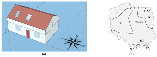
Figure 1.
(a) Model of the test building; (b) location of the building (I–V—climatic zones).
The building was designed to fulfil Polish guidelines for passive and low-energy buildings introduced by the National Fund for Environmental Protection and Water Management, defining low-energy and passive buildings as having calculated annual usable energy for heating and ventilation EU = 40 kWh/m2 (also called NF40) and EU = 15 kWh/m2 (NF15), respectively [69,70,71,72,73]. External walls are from ceramic blocks insulated with 10 cm of Styrofoam. The attic is insulated with 15 cm of mineral wool. The ground floor is insulated with 20 cm layer of Styrofoam. Ventilation airflow was set at 150 m3/h on the basis of Polish requirements [74,75].
2.2. Ground Temperature
The basis for the EAHE design is the ground temperature at the burial depth. It can be estimated in several ways presented in recent decades by various authors. Carslaw and Jaeger [76] derived the equation of ground temperature at the given depth as a solution of the solution of the heat conduction equation in a semi-infinite medium under several assumptions [77,78,79]:
- The ground is treated as a semi-infinite medium with constant thermal diffusivity;
- The ground is a homogenous and anisotropic medium with respect to thermal conductivity;
- The ground surface temperature varies periodically over time;
- The model does not take into account the periodical occurrence of snow cover on the surface of the ground;
- The effect of EAHE operation on the ground temperature distribution was neglected.
That model was also applied in the EN 16798-5-1 standard [56] which describes a detailed calculation method for energy requirements of ventilation and air conditioning systems using an hourly calculation step. Among other areas, the method also covers ground pre-heating and pre-cooling. The mathematical model of ground temperature and EAHE given in EN 16798-5-1 was used in this study.
According to EN 16798-5-1 hourly ground temperature is given by the equation:
with:
and:
2.3. Earth-to-Air Heat Exchanger
The design aspects of EAHEs have been presented recently in numerous papers [31,37,39,44,80,81,82]. Based on them, as well as on the works showing cases from Poland, there were assumed parameters of EAHE, given in Table 1. Assuming pipe wall thickness of 8.8 mm the calculated area of the inner surface of the ground heat exchanger is As = 28.65 m2.

Table 1.
Parameters of the earth-to-air heat exchanger.
Having known ground temperature and basic parameters of EAHE the difference between the EAHE inlet and outlet air temperature can be obtained:
The overall heat transfer coefficient of EAHE is given by:
The inside surface heat transfer coefficient is calculated from:
To avoid iterative computations when applying Equation (6) the standard indicates the possibility to set Tmd = Te.
Finally, heating and cooling capacity of the heat exchanger can be obtained from the relationship [83]:
It can be also interpreted as additional heat flux added to air passing the exchanger.
2.4. The 5R1C Model
The thermal network model of a building zone, introduced by the EN ISO 13790 standard, consists of five resistors and one capacitor (Figure 2a).
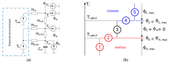
Figure 2.
The 5R1C thermal network model of a building zone from EN ISO 13790: (a) circuit diagram of the model; (b) control strategy to maintain required set-point temperatures.
The building shell is divided into two parts. Thermally “light” building elements, such as doors, windows, curtain walls and glazed walls, are described by the Htr,w thermal transmission coefficient. Thermally “heavy” opaque building elements, such as walls or ceilings, are described by the Htr,op thermal transmission coefficient. It is split into the external (Htr,em) and the internal (Htr,ms) parts. These parts are both connected to the thermal capacity (Cm), representing the thermal mass of the building [84]. On the other side, Htr,op and Htr,em coefficients are connected with the external temperature (Te). The heat transfer by ventilation (Hve) is connected with the supply air temperature (Tsup) and the internal air temperature (Ti). The latter one and the central node (Ts) are linked through the coupling conductance Htr,is.
The heat flow rates due to internal heat sources (φint) and due to solar heat sources (φsol) are split into three parts: φia, φst, and φm, connected to the indoor air, the central node, and the thermal mass temperature nodes, respectively. The heating or cooling power (φHC) is supplied to or extracted from the indoor air node.
Computations are performed in hourly time step. In each time step there is computed sensible heating or cooling power (φHC) required to maintain a certain set-point indoor air temperature: Tint,H,set or Tint,C,set for heating or cooling, respectively. There is also the possibility to control the required operative indoor air temperature instead.
To maintain required indoor air (or operative) temperature within a set range there is a need to supply proper heating or cooling power, φHC. EN ISO 13790 provides a suitable calculation procedure to obtain hourly values of φHC depending on the current conditions. Five situations, numbered from 1 to 5 in Figure 2b, may take place at the given time step during calculations:
- (1)
- The considered building (or zone) requires heating and the calculated hourly heating power (φH) is greater than the maximum available heating power, φH,max. Hence, the heating power φH = φH,max and the resulting internal air temperature is lower than the heating set-point Ti,set,H.
- (2)
- The building requires heating and the heating power is sufficient (φH < φH,max). The calculated internal air temperature is equal to Ti = Ti,set,H.
- (3)
- Neither heating nor cooling is required. The internal air temperature is calculated.
- (4)
- The building requires cooling and the cooling power is sufficient (φC < φC,max). The calculated internal air temperature is equal to Ti = Ti,set,C.
- (5)
- The building requires cooling and the calculated cooling power (φC) is greater than the maximum available heating power, φC,max. Hence, the cooling power φC = φC,max and the resulting internal air temperature is lower than the heating set-point Ti,set,C.
That procedure also has been presented recently in detail in various applications by several authors [85,86]. It can be easily implemented in a spreadsheet [87,88,89,90,91,92], which makes it very flexible.
In the studied case the supply air temperature is the outlet air temperature from the heat exchanger. Hence:
Ventilation heat transfer coefficient was computed from the relationship:
Applying the above to the circuit diagram from Figure 2a the ventilation heat flux can be obtained:
Equation (10) shows that, depending on the mutual relationship between Tsup and Ti and on the season of the year, there may occur favourable and unwanted phenomena related to the heat exchange between the surroundings and the building zone through ventilation. Such an analysis performed with regard to the model presented in Figure 2a is based on the heat flux balance in the internal air node “i”. Hence, heat flux has a positive sign when heat is supplied into that node and negative when heat is extracted.
When Tsup > Ti (and φve > 0) then ventilation air supplied to the building warms up its interior. During the cooling season, when and φHC < 0, it is a negative phenomenon resulting in increased cooling demand. However, when heating is needed, and φHC > 0, it reduces heating demand. The opposite takes place when Tsup < Ti. Then, ventilation air supplied to the building cools it down (φve < 0), reducing cooling needs during the cooling period and increasing heating demand during the heating period. As one can see, the sum of the heat fluxes φHC + φve provides information about their interaction and may be used as an indicator of ventilation influence on hourly thermal demand of a heating/cooling system.
In the considered example of EAHE supplying ventilation air to the building, varying outdoor and indoor conditions may create situations when the direct supply of outdoor air at Te temperature will be more beneficial than the air delivered from the heat exchanger and vice versa. For these reasons it was recommended to use an additional bypass to switch intake of ventilation air between EAHE and outdoor air [51]. Then, Tsup can be changed into Te when needed:
To include this possibility into the calculation procedure presented above an additional calculation algorithm was developed (Figure 3). However, some explanation is given first. Thermal power, φHC, supplied to the indoor air node, Ti, at current n-th time step depends on outdoor and indoor conditions. Among them, outdoor air and supply air temperatures are used to obtain required φHC. On the other hand, to select an appropriate ventilation air source (EAHE at Tsup or outdoor air at Te) at the same time step there should be known indoor thermal conditions given by Ti determining if heating or cooling is needed (Figure 2b). Hence, to avoid circular references in spreadsheet calculations there was assumed that the need of heating or cooling is checked in the previous (n-1) time step and then the selection procedure is to be continued (Figure 3). This simplification should not introduce large errors, because the temperature inside the building varies within a limited, fairly narrow range.
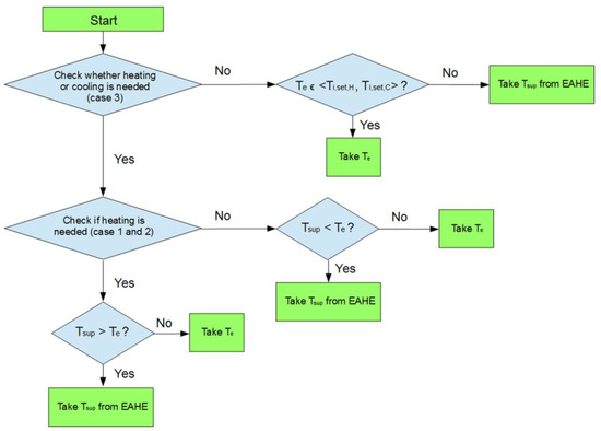
Figure 3.
Control algorithm for a bypass to select supply air between ambient air and an EAHE outlet.
When neither heating nor cooling is needed and external air temperature is within the range between Ti,set,H and Ti,set,C then outdoor temperature is chosen. That choice is based on the fact that EAHE requires fan operation, which generates additional costs. Of course, that algorithm can be modified following various assumptions.
This model is intended in calculations of sensible energy use for space heating and cooling. Therefore, it can be assumed that an all-air system provides both heating and cooling in the considered building. Humidification and dehumidification of air is not considered here. Hence, condensation in the buried pipe was not analysed.
3. Results and Discussion
3.1. Simulation Assumptions
3.1.1. Selection of a Reference Weather Station
To perform hourly simulations for the considered location the relevant meteorological hourly data are needed. As there are no such data for Gorlice city, the two closest meteorological stations were taken into account: Nowy Sącz (49°37′ N and 20°42′ E) and Krosno (49°43′ N and 21°46′ E). They are shown in Figure 1b. The first one is located 40 km west of Gorlice and the second one is located 50 km east of the considered city.
To choose one of them, and analysis was conducted at first. For comparison, measurements taken in the year 2020 in Gorlice were used. They were performed using three DS18B20 temperature sensors located about 1 m from an external wall of a residential building. The first one, used for external air temperature measurement, was placed in a radiation shield to reduce the impact of solar radiation. The second sensor was placed on a ground surface. The third one was buried in the ground at a depth of 1 m. The data were saved in 10 min intervals during the whole 2020 year.
First, outdoor air temperature for both meteorological stations from TMYs (TMY Nowy Sącz and TMY Krosno) and mean monthly air temperature measured in meteorological stations in 2020 (Nowy Sącz 2020 and Krosno 2020) and finally in the test location in Gorlice (Figure 4) were compared. External air temperature was taken from typical meteorological years freely available for 61 weather stations in Poland in hourly and monthly format [93,94].
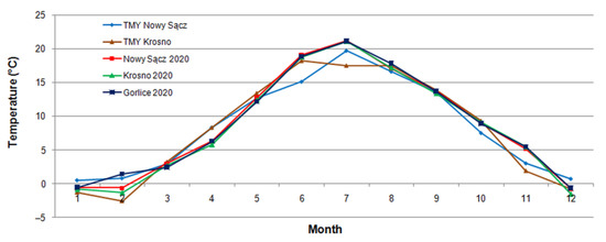
Figure 4.
Outdoor air temperature from TMYs and measured in 2020 year.
Good agreement was noticed when comparing data from the same year, 2020. In the case of TMYs, better fitting determined by the mean squared error (MSE) was observed for Nowy Sącz (2.77 K2) against 4.13 K2 for Krosno. Root mean square error (RMSE) was 1.66 K and 2.03 K in the same order. The same tendency followed for temperature in 2020: 0.46 K2 and 0.77 K2 for MSE and 0.68 K and 0.87 K for RMSE in Nowy Sącz and Krosno, respectively. Hence, for further simulations TMY for the Nowy Sącz station was chosen. Annual variation of air temperature and global solar irradiance in this station in hourly time step is presented in Figure 5.
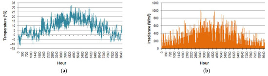
Figure 5.
TMY for Nowy Sącz: (a) outdoor air temperature; (b) global horizontal irradiance.
3.1.2. Ground Temperature
In the next step the model of ground temperature of EN 16798-5-1 given by Equation (1) was evaluated. Theoretical results provided by that model for the depth of 1 m were compared with measurements performed in Gorlice. Moist clay was assumed in the considerations. For this type of soil, according to EN 16798-5-1, λgnd = 1.45 W/(m∙K), ρgnd = 1800 kg/m3, and cgnd = 1340 J/(kg∙K). Results, in the form of monthly averaged values, are presented in Figure 6a. Tgnd,measured is the ground temperature from measurements described in the previous section. Tgnd is the ground temperature calculated from Equation (1) on the basis of monthly air temperature measured in 2020. Significant differences in winter months can be noticed. Hence, in the next step instead of outdoor air temperature, measured ground surface temperature was used. It was higher because of snow cover presence during that period. The resulting ground temperature, Tgnd,corr, was little higher than in the previous case, but still visible discrepancies occurred. Finally, for comparative purposes, measured outdoor air temperature and moist soil (λgnd = 1.50 W/(m∙K), ρgnd = 1400 kg/m3, cgnd = 1400 J/(kg∙K)) was used.
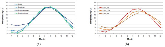
Figure 6.
Ground temperature: (a) calculated from measurements at the depth of 1 m; (b) calculated from TMY.
As results are comparable to those from the first case it was assumed that resulting differences between the model and measurements may arise from simplifications in the model [24,77,79,95,96,97]. In addition, the influence of the building’s neighbourhood may be taken into account [98]. As this problem is not the issue of the paper and good agreement was obtained for warm months, the model of EN 16798-5 was used in further calculations.
As usually burial depths presented in the literature varied between 1.1 m to 2.5 m, its impact on ground temperature (Figure 6b) was also simulated using monthly air temperature from TMY. Taking into account previous Polish studies the depth of 2.0 m was chosen for further considerations. It offers better thermal conditions for the analysed application than the two other depths: higher ground temperatures during cold months and lower during warm periods.
3.1.3. Thermal Model of the Building
For simulation purposes, the values of thermal conductance and single capacitance of the test building model from Figure 2 and given in Table 2 were calculated using the data of the materials obtained from manufacturers and from EN ISO 10456 [99]. Thermal resistances were calculated following ISO 6946 [100]. Thermal bridges were neglected. Thermal capacities were calculated according to the detailed method of ISO 13786 [101] for a calculation period of 24 h. Solar absorptance of the roof and wall surfaces was α = 0.8 and α = 0.6, respectively.
Table 2.
Thermal network model elements of the building.
According to EN ISO 13790 indications the volumetric heat capacity of air was assumed to be constant at ρaca = 1200 J/m3K, as in other building simulations [84,102,103]. From this (see Equation (9)) Hve = 50.0 W/K.
Internal gains were assumed to be constant (300 W) during the presence of occupants in the building, i.e., on working days except the period from 8:00 to 16:00, during weekends except the period from 8:00 to 16:00 from May to September, and 24 h/day during remaining weekends from October to April. Ventilation was switched on with constant airflow qv;sup = 150 m3/h only during the presence of occupants in the building. Three cases were simulated, as follows:
- No EAHE, Tsup = Te (only natural ventilation);
- EAHE working without a bypass;
- EAHE working with an additional bypass.
3.2. Simulation Results
Annual effectiveness of the analysed heat exchanger during its continuous operation during a year can be characterised by various indicators. The first of them is the air temperature rise, ΔTsup, presented in Figure 7.
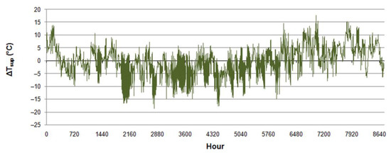
Figure 7.
Air temperature change in the heat exchanger.
This quantity characterises the operation mode of the EAHE. If ΔTsup < 0 then inlet outdoor air passing the exchanger is cooled, which takes place in summer months. Otherwise, air is warmed up, and it can be observed during the first half of January when low air temperature is noticed (Figure 5a).
ΔTsup varied from −18.7 °C on 27 April at 12:00 to 17.6 °C on 19 October at 6:00. Monthly averaged ΔTsup was from 0.27 °C in February to 4.98 °C in November and from −0.72 °C in August to −3.96 °C in May.
Congedo et al. [29] simulated (ANSYS Fluent) an air–ground heat exchanger built from a 5 m long single polyethylene (PEX) and polypropylene (PP) pipe with an air flow rate of 150 m3/h, located in the predominantly hot and humid climate of southern Italy. For the coldest winter week, the pre-heating effect was almost unnoticeable. In summer the average temperature gain was between 2 °C and 3 °C.
In the analysed case the total monthly heat gain was from 9.18 kWh in February to 179.18 kWh in November and from −26.93 kWh in August to −171.97 kWh in July. These values, however, do not provide full information as they were obtained summing heating and cooling heat fluxes because of bidirectional hourly heat flows occurring during longer periods, such as weeks or months. More reliable is hourly heating and cooling capacity of the exchanger, φEAHE, which varied from −933.7 W to 880.8 W on the same days as ΔTsup. According to Equation (7) it followed changes of ΔTsup.
Skotnicka et al. [53] presented data from a laboratory experiment on an air-to-soil heat exchanger performance conducted from 1 July to 30 September 2016 in Olsztyn (north Poland). The exchanger consisted of 41 m long PP (polypropylene) pipes with 0.2 m diameter buried at depths from 2.1 m to 2.28 m. Empirical data were compared with the results of analytical calculations based on TMY for Olsztyn.
The maximum hourly heat gain was 0.29 kWh and 0.73 kWh in the experiment and in theoretical calculations, respectively. The maximum measured and calculated hourly cooling load was −0.16 kWh and −0.65 kWh, respectively. Monthly heat gain from measurements amounted to 37.24 kWh, 62.42 kWh and 82.41 kWh in July, August and September, respectively. The same from calculations was 44.00 kWh, 58.27 kWh and 95.22 kWh. More significant discrepancies were noticed in the case of cooling. Measured monthly cooling energy was −6.42 kWh, −4.45 kWh and −1.35 kWh in the consecutive months. Calculations resulted in −57.58 kWh, −79.92 kWh and −88.32 kWh. Due to the authors’ low measured values, cooling energy could result from the permanent (24 h/day) operation of fans in spring, which rose the ground temperature.
Recently [103] there have been presented results of a three-year monitoring campaign of the EAHE performance in the same location. Various ventilation strategies in a modern single-storey residential building, with a usable floor area of 115 m2, were analysed. The building was equipped with a gravity ventilation system. Design ventilation airflow was established at 150 m3/h, i.e., 0.5 air changes per hour. Calculations performed on the basis of measurements showed that the exchanger provided hourly 257.6 W and 124.7 W of heating and cooling power, respectively. Because of climatic conditions the system operated mainly in the heating mode. Annual ventilation heat loss was reduced by about 45%.
Correlation of the working mode of EAHE with regard to outdoor conditions is presented in Figure 8. Inlet air was cooled for outdoor temperatures higher than about 1 °C. For better clarity, hourly results are presented for warm (IV–IX) and cold (X–III) months with green and brown colours, respectively. As expected, pre-heating (ΔTsup > 0) dominated in colder and pre-cooling with ΔTsup < 0 in warmer months. However, one should remember that this is only an illustration of a possible situation. Utilisation of outlet air depends only on the user’s requirements and the HVAC system’s setup, as described in Section 2.
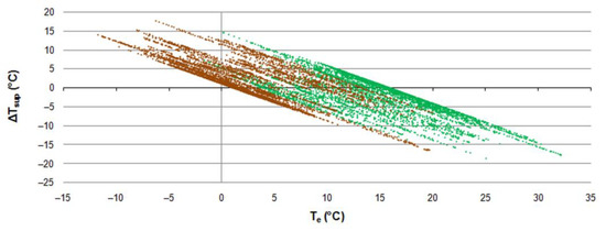
Figure 8.
The air temperature difference in EAHE in relation to ambient air temperature.
Calculated hourly ground temperature was from 0.96 °C (10–13 February) to 15.94 °C (12–15 August). Its variation was followed by the next important parameter describing EAHE operation, which is outlet air temperature (Tsup), given in Figure 9. It was calculated using weather data from TMY in the considered location and the calculation procedure described in Section 2. Monthly averaged Tsup was from 0.77 °C in February to 19.65 °C in July. Hourly Tsup varied from 0.94 °C on 10 February at 6:00 to 15.86 °C on 15 August at 14:00 and it differed from Tgnd up to ±0.2 °C.
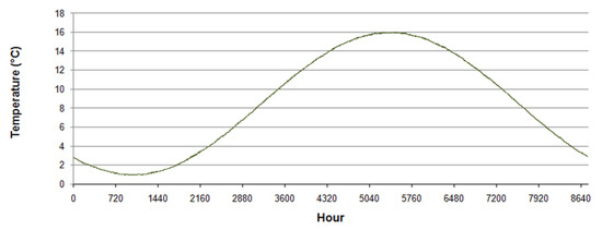
Figure 9.
Outlet air temperature from the earth-to-air heat exchanger.
Annual sensible heating and cooling demand of the building in the first case, without the EAHE, was 14.82 GJ and 1.67 GJ, respectively. Hence, the total unit energy use for space heating and cooling was EA = 34.7 kWh/m2.
Monthly demand varied from 0.11 GJ in September to 3.18 GJ in December and from 0.07 GJ in April to 0.70 GJ in July, for heating and cooling, respectively. Maximum hourly thermal power was 2.73 kW on 8 January at 7:00 and 3.06 kW on 21 July at 15:00 in the same order (Figure 10).
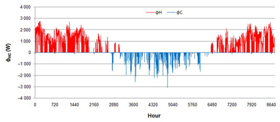
Figure 10.
Hourly heating and cooling power in case 1.
The heating system was working for 4010 h during the year (Figure 11a). The dominating power requirement was up to 1000 W (1841 h). For 432 h heating power was greater than 2000 W. Cooling worked for 1404 h (Figure 11b), from which for 1030 h was with a load lower than 500 W.
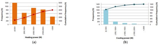
Figure 11.
Histograms in case 1: (a) heating power; (b) cooling power.
As can be seen in Figure 12, in the analysed case natural ventilation resulted in increased heating demand during the cold season when the outdoor air temperature was low (Figure 5a).
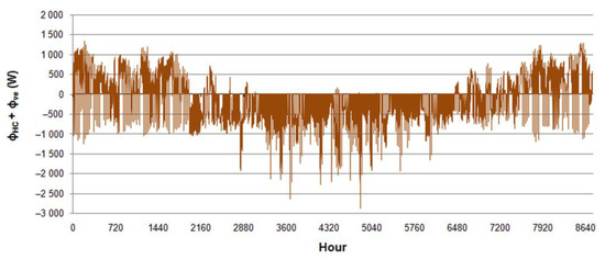
Figure 12.
Impact of ventilation heat flux on the heating and cooling power in case 1.
Negative peak values in that period appeared because of assumed intermittent operation of the ventilation system. When it was turned off, the building structure was at such a temperature that it was not necessary to heat the building up for several hours until the ventilation was turned on again. In the first hour after turning on the ventilation again, a negative ventilation heat flux appeared. In the next hour it was necessary to supply heat for heating and the sum φHC + φve changed its sign. During the rest of the year, in spring and summer, the high outdoor air temperature resulted in overheating of the building and increased cooling demand.
In the second analysed case, when EAHX was used instead of natural ventilation, monthly demand varied from 0.06 GJ in September to 2.75 GJ in December and from 0.01 GJ in April to 0.44 GJ in July, for heating and cooling, respectively. Compared to the previous case, annual heating and cooling energy decreased by 1.66 GJ to 13.16 GJ and by 0.72 GJ to 0.95 GJ, i.e., by 11.2% and 43.2%, respectively. Consequently, the EA indicator was lower by 5.0 kWh/m2 and amounted to 29.7 kWh/m2 (by 21.2%). In addition, the hourly peak power decreased by 0.52 kW to 2.21 kW on 2 February at 7:00 and by 0.75 kW to 2.31 kW on 21 June at 15:00 in the same order (Figure 13).
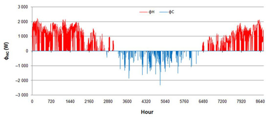
Figure 13.
Hourly heating and cooling power in case 2.
Heating power was supplied to the building for 4092 h during the year (Figure 14a). The dominating power requirement was up to 1000 W (2085 h). For 62 h heating power was greater than 2000 W. Cooling worked for 1250 h (Figure 14b), from which for 1043 h was with a load lower than 500 W.
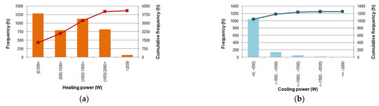
Figure 14.
Histograms in the second case: (a) heating power; (b) cooling power.
In the study [31] for Stockholm in Sweden authors simulated EAHE built from 10 m long polyethylene pipe of 20 cm diameter, buried at 2 m. The estimated annual energy saving for the base case, with a ventilation air flow rate of 60 dm3/s, amounted to 525 kWh and 300 kWh for the heating and cooling season, respectively. It was 5% for heating and 50% for cooling compared to if no EAHE was used.
The last examined was the third case with EAHE and additional bypass controlled following the developed control algorithm presented in Figure 3. As noticed, to avoid circular references, supply air temperature at the n-th time step was chosen from thermal conditions (φHC) at the previous n-1 time step.
This time, the differences in relation to the previous case were not significant. However, several positive effects can be seen. Operation of the bypass resulted in switching between two sources of ventilation air entering the building of different values (Te and Tsup), presented in Figure 15. It was especially visible during the heating period.
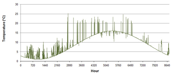
Figure 15.
Supply air temperature Tsup in the case of the bypass operation (3rd case).
Monthly demand varied from 0.06 GJ in September to 2.69 GJ in December and from 0.01 GJ in April to 0.45 GJ in July, for heating and cooling, respectively. Compared to the previous case, annual heating decreased by 0.44 GJ to 12.76 GJ. Annual cooling increased slightly by 0.01 GJ to 0.91 GJ. Consequently, the EA indicator was lower by 0.8 kWh/m2 and amounted to 28.9 kWh/m2. The hourly peak power remained the same.
The heating system worked for 4053 h which is 34 h less (Figure 16a) than in the second case. The dominating power requirement was up to 1000 W (2137 h). For 62 h heating power was greater than 2000 W. Cooling worked for 1270 h, i.e., 14 h more (Figure 16b), from which for 1053 h (15 h more) was with a load below 500 W.
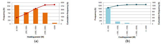
Figure 16.
Histograms in the third case: (a) heating power; (b) cooling power.
In the same case, but using iterative calculations, the annual heating and cooling demand decreased by 0.06 GJ and 0.06 GJ to 12.74 GJ and 0.93 GJ, respectively. The EA indicator was 25.8 kWh/m2. Hourly peak power, both for heating and cooling, remained the same, but the dynamics of the bypass control was improved, and several switching cycles were avoided. Especially in hot months under free float conditions, when at a certain hour (say, n-th) cooling was not required on the basis of the thermal condition at the previous hour (n-1), but simultaneously the system supplied ventilation air at Te higher than the outlet from EAHE, creating the need for cooling at the n-th hour. Hence, the number of peaks observed in Figure 17 decreased in reference to Figure 15.
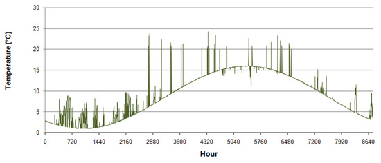
Figure 17.
Supply air temperature Tsup in the case of the bypass operation—calculations with circular references.
The thermal effect was not very significant (in Table 3 assigned as “Case 3 i”), but it indicated that the problem mentioned by other authors [46,48] is of practical importance and worthy of further consideration. It also should be noted here that 123 kWh of savings between case two and case three i (iterative calculations) are 3.3% of the total heating and cooling consumption in case two.
Table 3.
Calculated annual energy use for space heating and cooling in the studied cases.
Total percentage annual heating and cooling energy savings, ΔQHC, given in Table 3, were calculated in relation to case one.
The obtained savings (up to 17%) are not significant when compared to other European studies. This may be due to various reasons. The first one is the type of the considered object. As a low-energy building was the base case, further improvements resulted in a lower level of savings than for traditional, non-modernised buildings.
The second factor is linked with climatic conditions in the analysed locations. For predominantly hot and humid climatic conditions of southern Italy [29], authors concluded that in the case of a 100 m2 building, with average insulation, from about 1.000 kWh/year for space heating and cooling 50% can be covered by the system of EAHE with three 20 m long pipes. Similar outcomes were given in [45], where authors stated that EAHE is preferable in hot or mild climates. The combination of EAHE and air-to-air heat exchanger (AAHE) resulted in savings of 75% and 60% in Milan and Palermo, respectively. For Spanish conditions [104], authors estimated, using the TRNSYS tool, annual energy savings at 10.5% and 25.1% for heating and cooling, respectively. On the other hand, based on measurements of an EAHE located in north Poland it was reported in [55] that for a low-energy residential building, there were given annual savings of around 20% and 3%.
As stated in Section 2, the effect of EAHE operation on the ground temperature distribution was neglected, but periodical operation of EAHE assumed in the paper reduced this impact to a certain limit.
The presented control algorithm is an attempt to introduce an EAHE bypass control in hourly dynamic modelling of buildings using the very well-known and well-funded 5R1C thermal network model of a building zone.
4. Conclusions
In this study, annual operation of the earth-to-air heat exchanger (EAHE) supplying ventilation air to the low-energy residential building, according to Polish regulations, was studied. To include hourly variation of the building use and climatic conditions the 5R1C thermal network model of a building zone from the EN ISO 13790 standard was used. Calculations of the EAHE performance were performed following the EN 16798-5-1 standard. The developed algorithm to choose the source of ventilation air supplied to the building between the EAHE output and outdoor air showed its applicability. All simulations were performed in a spreadsheet not requiring the use of commercial, sophisticated tools.
Application of EAHE in Polish conditions was confirmed. In the first case, where only natural ventilation was assumed, annual energy use for space heating and cooling was 16.48 GJ. Application of EAHE decreased it by 14.4% to 14.11 GJ. In the third case, where the developed control algorithm to switch between EAHE and natural ventilation was applied, total consumption decreased to 13.73 GJ, i.e., by 16.7% when compared to the first case. Application of circular references to the third case in the calculation procedure revealed that several switching cycles between EAHE and natural ventilation were avoided and further lowering of heating and cooling needs to 13.67 GJ were reached. In this value, the proposed bypass allowed to save 443 MJ, which was 3.3% of the total consumption when only EAHE operation was considered.
Another important fact is that peak hourly heating and cooling thermal power decreased from 2.73 kW and 3.06 kW to 2.21 kW and 2.34 kW. On the other hand, annual operation time of heating and cooling changed from 4010 h and 1404 h to 4063 h and 1228 h, respectively, which mean the method offered more stability in operation.
Of course, it should be remembered that several modelling assumptions were made. The effect of EAHE operation on the ground temperature distribution was neglected and energy consumption by fans was not taken into account. Therefore, these and other factors may be taken into consideration in further investigations.
Funding
This research received no external funding.
Institutional Review Board Statement
Not applicable.
Informed Consent Statement
Not applicable.
Data Availability Statement
Not applicable.
Conflicts of Interest
The author declares no conflict of interest.
Abbreviations
| As | inner surface of the ground heat exchanger, m2 |
| Cm | thermal capacity of the building, J/K |
| EA | unit heating and cooling energy use per unit area of a building, kWh/m2 |
| EU | annual usable energy for heating and ventilation, kWh/m2 |
| Htr,em | external part of the Htr,op thermal transmission coefficient, W/K |
| Htr,is | coupling conductance, W/K |
| Htr,ms | internal part of the Htr,op thermal transmission coefficient, W/K |
| Htr,op | thermal transmission coefficient for thermally heavy envelope elements, W/K |
| Htr,w | thermal transmission coefficient for thermally light envelope elements, W/K |
| Hve | thermal transmission coefficient by ventilation air, W/K |
| L | length of the duct, m |
| QC | annual energy use for space cooling, kWh |
| QH | annual energy use for space heating, kWh |
| QHC | annual energy use for space heating and cooling, kWh |
| ΔQHC | percentage savings in annual energy use for space heating and cooling, % |
| Te | external (outdoor) air temperature, °C |
| Te;mn;an | mean annual temperature of outdoor air, °C |
| Te;max;m | maximum mean monthly temperature of outdoor air, °C |
| Tgnd | hourly ground temperature, °C |
| Ti | internal (indoor) air temperature, °C |
| Ti,C,set | set-point indoor air temperature for cooling, °C |
| Ti,H,set | set-point indoor air temperature for heating, °C |
| Tm | thermal mass node temperature, °C |
| Tmd | average air temperature in the duct, °C |
| Ts | central node temperature, °C |
| Tsup | supply air temperature, °C |
| ca | specific heat of air at constant pressure, J/(kg∙K) |
| cgnd | specific heat of the ground, J/(kg∙K) |
| di | inner diameter of the duct, m |
| do | outer diameter of the duct, m |
| ft | time shift factor, — |
| hi | inside surface heat transfer coefficient, W/m2K |
| qv;sup | volumetric airflow rate, m3/s |
| tan | annual hour, with tan = 0 h at the beginning of the year, h |
| tan;min | the time of the year when the monthly mean outdoor temperature is minimal, h |
| v | air velocity in the duct, m/s |
| z | burial depth of the duct, m |
| λgnd | thermal conductivity of the ground, W/(m∙K) |
| λdu | thermal conductivity of the duct, W/(m∙K) |
| ξ | damping factor, — |
| ρa | air density, kg/m3 |
| ρgnd | ground density, kg/m3 |
| φint | heat flow rate due to internal heat sources, W |
| φsol | heat flow rate due to solar heat sources, W |
| φia | heat flow rate to internal air node, W |
| φst | heat flow rate to central node, W |
| φm | heat flow rate to mass node, W |
| φve | heat flow rate by ventilation, W |
| φEAHE | heat flow rate from EAHE, W |
| φC | cooling power supplied to or extracted from the indoor air node, W |
| φH | heating power supplied to or extracted from the indoor air node, W |
| φHC | heating or cooling power supplied to or extracted from the indoor air node, W |
References
- BPIE. Europe’s Buildings under the Microscope. 2011. Available online: https://www.bpie.eu/wp-content/uploads/2015/10/HR_EU_B_under_microscope_study.pdf (accessed on 22 February 2022).
- D’Agostino, D.; Cuniberti, B.; Bertoldi, P. Energy consumption and efficiency technology measures in European non-residential buildings. Energy Build. 2017, 153, 72–86. [Google Scholar] [CrossRef]
- Ramczyk, M. Legal bases and economic conditions of applying renewable energy resources in construction industry. MATEC Web Conf. 2018, 174, 04004. [Google Scholar] [CrossRef][Green Version]
- Dołęga, W. Selected aspects of national economy energy efficiency. Energy Policy J 2019, 22, 19–32. [Google Scholar] [CrossRef]
- Jezierski, W.; Sadowska, B.; Pawłowski, K. Impact of Changes in the Required Thermal Insulation of Building Envelope on Energy Demand, Heating Costs, Emissions, and Temperature in Buildings. Energies 2021, 14, 56. [Google Scholar] [CrossRef]
- Papadopoulos, A.M.; Papageorgiou, K.P.; Karatzas, K. Evaluation of an attached sunspace without sun protection: How feasible is this approach in mediterranean summer conditions? Int. J. Sol. Energy 2002, 22, 93–104. [Google Scholar] [CrossRef]
- Bekkouche, S.M.A.; Benouaz, T.; Hamdani, M.; Cherier, M.K.; Yaiche, M.R.; Benamrane, N. Diagnosis and comprehensive quantification of energy needs for existing residential buildings under Sahara weather conditions. Adv. Build. Energy Res. 2007, 11, 37–51. [Google Scholar] [CrossRef]
- Witkowska, A.; Krawczyk, D.A.; Rodero, A. Investment Costs of Heating in Poland and Spain—A Case Study. Proceedings 2019, 16, 40. [Google Scholar] [CrossRef]
- Chwieduk, D.; Chwieduk, M. Determination of the Energy Performance of a Solar Low Energy House with Regard to Aspects of Energy Efficiency and Smartness of the House. Energies 2020, 13, 3232. [Google Scholar] [CrossRef]
- Kostka, M.; Szulgowska-Zgrzywa, M. Change-over natural and mechanical ventilation system energy consumption in single-family buildings. ASEE17 E3S Web Conf. 2017, 22, 00086. [Google Scholar] [CrossRef]
- Xu, Q.; Riffat, S.; Zhang, S. Review of Heat Recovery Technologies for Building Applications. Energies 2019, 12, 1285. [Google Scholar] [CrossRef]
- Kostka, M. Hybrid ventilation in residential buildings—The proposal of research for the Polish climatic conditions. E3S Web Conf. 2017, 17, 00043. [Google Scholar] [CrossRef]
- Fidorów-Kaprawy, N.; Kostka, M.; Szulgowska-Zgrzywa, M.; Piechurski, K. The energy concept of the building as a part of sustainable construction. Architectus 2017, 49, 115–130. [Google Scholar] [CrossRef]
- Gagliano, A.; Nocera, F.; Patania, F.; Moschella, A.; Detommaso, M.; Evola, G. Synergic effects of thermal mass and natural ventilation on the thermal behaviour of traditional massive buildings. Int. J. Sustain. Energy 2016, 35, 411–428. [Google Scholar] [CrossRef]
- Michalak, P.; Szczotka, K.; Szymiczek, J. Energy Effectiveness or Economic Profitability? A Case Study of Thermal Modernization of a School Building. Energies 2021, 14, 1973. [Google Scholar] [CrossRef]
- Tisov, A.; Dedeoglu, A.; Willems, E.; Visser, L.; Op’t Veld, P. Sets of Deep Renovation Solutions of Buildings HVAC Systems. Deliverable Report D1.3. 2017. Available online: https://ec.europa.eu/research/participants/documents/downloadPublic?documentIds=080166e5b82e1276&appId=PPGMS (accessed on 22 February 2022).
- Nowak-Dzieszko, K.; Rojewska-Warchał, M. Thermal comfort of the individual flats of multi–family panel building. Tech. Trans. Civ. Eng. 2014, 201–206. [Google Scholar] [CrossRef]
- Orzechowski, T.; Orzechowski, M. Energy savings due to building insulation of different thickness. E3S Web Conf. 2017, 14, 01030. [Google Scholar] [CrossRef]
- Bajno, D.; Bednarz, Ł.; Grzybowska, A. The Role and Place of Traditional Chimney System Solutions in Environmental Progress and in Reducing Energy Consumption. Energies 2021, 14, 4720. [Google Scholar] [CrossRef]
- Kang, E.-C.; Lee, E.-J.; Ghorab, M.; Yang, L.; Entchev, E.; Lee, K.-S.; Lyu, N.-J. Investigation of Energy and Environmental Potentials of a Renewable Trigeneration System in a Residential Application. Energies 2016, 9, 760. [Google Scholar] [CrossRef]
- D’Agostino, D.; Greco, A.; Masselli, C.; Minichiello, F. The employment of an earth-to-air heat exchanger as pre-treating unit of an air conditioning system for energy saving: A comparison among different worldwide climatic zones. Energy Build. 2020, 229, 110517. [Google Scholar] [CrossRef] [PubMed]
- Abbaspour-Fard, M.H.; Gholami, A.; Khojastehpour, M. Evaluation of an earth-to-air heat exchanger for the north-east of Iran with semi-arid climate. Int. J. Green Energy 2011, 8, 499–510. [Google Scholar] [CrossRef]
- Lee, K.-S.; Kang, E.-C.; Kim, Y.-J.; Lee, E.-J. Model Verification and Justification Study of Spirally Corrugated Pipes in a Ground-Air Heat Exchanger Application. Energies 2019, 12, 4047. [Google Scholar] [CrossRef]
- Leski, K.; Luty, P.; Gwadera, M.; Larwa, B. Numerical Analysis of Minimum Ground Temperature for Heat Extraction in Horizontal Ground Heat Exchangers. Energies 2021, 14, 5487. [Google Scholar] [CrossRef]
- Selamat, S.; Miyara, A.; Kariya, K. Analysis of Short Time Period of Operation of Horizontal Ground Heat Exchangers. Resources 2015, 4, 507–523. [Google Scholar] [CrossRef]
- Amanowicz, Ł.; Wojtkowiak, J. Validation of CFD model for simulation of multi-pipe earth-to-air heat exchangers (EAHEs) flow performance. Therm. Sci. Eng. Prog. 2018, 5, 44–49. [Google Scholar] [CrossRef]
- Rodríguez-Vázquez, M.; Hernández-Pérez, I.; Xamán, J.; Chávez, Y.; Noh-Pat, F. Computational Fluid Dynamics for Thermal Evaluation of Earth-to-Air Heat Exchanger for Different Climates of Mexico. In CFD Techniques and Thermo-Mechanics Applications; Driss, Z., Necib, B., Zhang, H.C., Eds.; Springer: Cham, Switzerland, 2018. [Google Scholar] [CrossRef]
- Boban, L.; Miše, D.; Herceg, S.; Soldo, V. Application and Design Aspects of Ground Heat Exchangers. Energies 2021, 14, 2134. [Google Scholar] [CrossRef]
- Congedo, P.M.; Lorusso, C.; De Giorgi, M.G.; Marti, R.; D’Agostino, D. Horizontal Air-Ground Heat Exchanger Performance and Humidity Simulation by Computational Fluid Dynamic Analysis. Energies 2016, 9, 930. [Google Scholar] [CrossRef]
- Agrawal, K.K.; Bhardwaj, M.; Misra, R.; Agrawal, G.D.; Bansal, V. Optimization of operating parameters of earth air tunnel heat exchanger for space cooling: Taguchi method approach. Geotherm. Energy 2018, 6, 10. [Google Scholar] [CrossRef]
- Havtun, H.; Törnqvist, C. Reducing Ventilation Energy Demand by Using Air-to-Earth Heat Exchangers. Part 1—Parametric Study. In Sustainability in Energy and Buildings; Hakansson, A., Höjer, M., Howlett, R., Jain, L., Eds.; Smart Innovation, Systems and Technologies; Springer: Berlin/Heidelberg, Germany, 2013; Volume 22. [Google Scholar] [CrossRef]
- Amanowicz, Ł.; Wojtkowiak, J. Thermal performance of multi-pipe earth-to-air heat exchangers considering the non-uniform distribution of air between parallel pipes. Geothermics 2020, 88, 101896. [Google Scholar] [CrossRef]
- Amanowicz, Ł.; Wojtkowiak, J. Approximated flow characteristics of multi-pipe earth-to-air heat exchangers for thermal analysis under variable airflow conditions. Renew. Energy 2020, 158, 585–597. [Google Scholar] [CrossRef]
- Amanowicz, Ł.; Wojtkowiak, J. Comparison of Single- and Multipipe Earth-to-Air Heat Exchangers in Terms of Energy Gains and Electricity Consumption: A Case Study for the Temperate Climate of Central Europe. Energies 2021, 14, 8217. [Google Scholar] [CrossRef]
- Al-Ismaili, A.M.; Fadel, M.A.; Jayasuriya, H.; Janitha Jeewantha, L.H.; Al-Mahdouri, A.; Al-Shukeili, T. Potential reduction in water consumption of greenhouse evaporative coolers in arid areas via earth-tube heat exchangers. J. Arid Land 2021, 13, 388–396. [Google Scholar] [CrossRef]
- Sakhri, N.; Menni, Y.; Chamkha, A.J.; Kaid, N. Experimental study of an earth-to-air heat exchanger coupled to the solar chimney for heating and cooling applications in arid regions. J. Anal. Calorim. 2021, 145, 3349–3358. [Google Scholar] [CrossRef]
- Havtun, H.; Törnqvist, C. Reducing Ventilation Energy Demand by Using Air-to-Earth Heat Exchangers. Part 2—System Design Considerations. In Sustainability in Energy and Buildings; Hakansson, A., Höjer, M., Howlett, R., Jain, L., Eds.; Smart Innovation, Systems and Technologies; Springer: Berlin/Heidelberg, Germany, 2013; Volume 22. [Google Scholar] [CrossRef]
- Tan, L.; Love, J.A. A Literature Review on Heating of Ventilation Air with Large Diameter Earth Tubes in Cold Climates. Energies 2013, 6, 3734–3743. [Google Scholar] [CrossRef]
- Chlela, F.; Husaunndee, A.; Riederer, P.; Inard, C. Numerical Evaluation of Earth to Air Heat Exchangers and Heat Recovery Ventilation Systems. Int. J. Vent. 2007, 6, 31–42. [Google Scholar] [CrossRef]
- Greco, A.; Masselli, C. The Optimization of the Thermal Performances of an Earth to Air Heat Exchanger for an Air Conditioning System: A Numerical Study. Energies 2020, 13, 6414. [Google Scholar] [CrossRef]
- Baglivo, C.; Bonuso, S.; Congedo, P.M. Performance Analysis of Air Cooled Heat Pump Coupled with Horizontal Air Ground Heat Exchanger in the Mediterranean Climate. Energies 2018, 11, 2704. [Google Scholar] [CrossRef]
- Baglivo, C.; D’Agostino, D.; Congedo, P.M. Design of a Ventilation System Coupled with a Horizontal Air-Ground Heat Exchanger (HAGHE) for a Residential Building in a Warm Climate. Energies 2018, 11, 2122. [Google Scholar] [CrossRef]
- Khabbaz, M.; Benhamou, B.; Limam, K.; Hollmuller, P.; Hamdi, H.; Bennouna, A. Experimental and numerical study of an earth-to-air heat exchanger for air cooling in a residential building in hot semi-arid climate. Energy Build. 2016, 125, 109–121. [Google Scholar] [CrossRef]
- Warwick, D.J.; Cripps, A.J.; Kolokotroni, M. Integrating Active Thermal Mass Strategies with HVAC Systems: Dynamic Thermal Modelling. Int. J. Vent. 2009, 7, 345–367. [Google Scholar] [CrossRef]
- D’Agostino, D.; Marino, C.; Minichiello, F. Earth-to-Air versus Air-to-Air Heat Exchangers: A Numerical Study on the Energetic, Economic, and Environmental Performances for Italian Office Buildings. Heat Transf. Eng. 2020, 41, 1040–1051. [Google Scholar] [CrossRef]
- D’Agostino, D.; Esposito, F.; Greco, A.; Masselli, C.; Minichiello, F. Parametric Analysis on an Earth-to-Air Heat Exchanger Employed in an Air Conditioning System. Energies 2020, 13, 2925. [Google Scholar] [CrossRef]
- D’Agostino, D.; Esposito, F.; Greco, A.; Masselli, C.; Minichiello, F. The Energy Performances of a Ground-to-Air Heat Exchanger: A Comparison among Köppen Climatic Areas. Energies 2020, 13, 2895. [Google Scholar] [CrossRef]
- Stasi, R.; Liuzzi, S.; Paterno, S.; Ruggiero, F.; Stefanizzi, P.; Stragapede, A. Combining bioclimatic strategies with efficient HVAC plants to reach nearly-zero energy building goals in Mediterranean climate. Sustain. Cities Soc. 2020, 63, 102479. [Google Scholar] [CrossRef]
- Żukowski, M.; Sadowska, B.; Sarosiek, W. Assessment of the cooling potential of an earth-tube heat exchanger in residential buildings. Environmental Engineering. In Proceedings of the 8th International Conference, Vilnius, Lithuania, 19–20 May 2011; Available online: http://citeseerx.ist.psu.edu/viewdoc/summary?doi=10.1.1.459.991 (accessed on 22 February 2022).
- Romańska-Zapała, A.; Furtak, M.; Dechnik, M. Cooperation of Horizontal Ground Heat Exchanger with the Ventilation Unit during Summer—Case Study. IOP Conf. Ser. Mater. Sci. Eng. 2017, 245, 052027. [Google Scholar] [CrossRef]
- Trząski, A.; Zawada, B. The influence of environmental and geometrical factors on air-ground tube heat exchanger energy efficiency. Build. Environ. 2011, 46, 1436–1444. [Google Scholar] [CrossRef]
- Łuczak, R.; Ptaszyński, B.; Kuczera, Z.; Życzkowski, P. Energy efficiency of ground-air heat exchanger in the ventilation and airconditioning systems. E3S Web Conf. 2018, 46, 00015. [Google Scholar] [CrossRef]
- Skotnicka-Siepsiak, A.; Wesołowski, M.; Piechocki, J. Experimental and Numerical Study of an Earth-to-Air Heat Exchanger in Northeastern Poland. Pol. J. Environ. Stud. 2018, 27, 1255–1260. [Google Scholar] [CrossRef]
- Skotnicka-Siepsiak, A.; Wesołowski, M.; Piechocki, J. Validating Models for Calculating the Efficiency of Earth-to-Air Heat Exchangers Based on Laboratory Data for Fall and Winter 2016 in Northeastern Poland. Pol. J. Environ. Stud. 2019, 28, 3431–3438. [Google Scholar] [CrossRef]
- Skotnicka-Siepsiak, A. Operation of a Tube GAHE in Northeastern Poland in Spring and Summer—A Comparison of Real-World Data with Mathematically Modeled Data. Energies 2020, 13, 1778. [Google Scholar] [CrossRef]
- EN 16798-5-1; Energy Performance of Buildings. Ventilation for Buildings Calculation Methods for Energy Requirements of Ventilation and Air Conditioning Systems (Modules M5-6, M5-8, M6-5, M6-8, M7-5, M7-8). Method 1: Distribution and Generation. The European Committee for Standardization: Brussels, Belgium, 2017.
- Romanska-Zapala, A.; Bomberg, M.; Dechnik, M.; Fedorczak-Cisak, M.; Furtak, M. On Preheating of the Outdoor Ventilation Air. Energies 2020, 13, 15. [Google Scholar] [CrossRef]
- Nunes, A.I.F.; Oliveira Panão, M.J.N. Passive Cooling Load Ratio method. Energy Build. 2013, 64, 209–217. [Google Scholar] [CrossRef]
- EN ISO 13790; Energy Performance of Buildings—Calculation of Energy Use for Space Heating and Cooling. International Organization for Standardization: Geneva, Switzerland, 2009.
- Elci, M.; Delgado, B.M.; Henning, H.M.; Henze, G.P.; Herkel, S. Aggregation of residential buildings for thermal building simulations on an urban district scale. Sustain. Cities Soc. 2018, 39, 537–547. [Google Scholar] [CrossRef]
- Lauster, M.; Teichmann, J.; Fuchs, M.; Streblow, R.; Mueller, D. Low order thermal network models for dynamic simulations of buildings on city district scale. Build. Environ. 2014, 73, 223–231. [Google Scholar] [CrossRef]
- Horvat, I.; Dović, D. Dynamic modeling approach for determining buildings technical system energy performance. Energy Convers. Manag. 2016, 125, 154–165. [Google Scholar] [CrossRef]
- Oliveira Panão, M.J.N.; Santos, C.A.P.; Mateus, N.M.; Carrilho da Graça, G. Validation of a lumped RC model for thermal simulation of a double skin natural and mechanical ventilated test cell. Energy Build. 2016, 121, 92–103. [Google Scholar] [CrossRef]
- Jayathissa, P.; Luzzatto, M.; Schmidli, J.; Hofer, J.; Nagy, Z.; Schlueter, A. Optimising building net energy demand with dynamic BIPV shading. Appl. Energy 2017, 202, 726–735. [Google Scholar] [CrossRef]
- Michalak, P. The development and validation of the linear time varying Simulink-based model for the dynamic simulation of the thermal performance of buildings. Energy Build. 2017, 141, 333–340. [Google Scholar] [CrossRef]
- Bertagnolio, S.; André, P. Development of an Evidence-Based Calibration Methodology Dedicated to Energy Audit of Office Buildings. Part 1: Methodology and Modeling. In Proceedings of the 10th REHVA World Congress–Clima, Anatalya, Turkey, 9–12 May 2010; Available online: https://orbi.uliege.be/bitstream/2268/29291/1/CLIMA10_HAC_paper1_SB100126.pdf (accessed on 22 February 2022).
- Fischer, D.; Wolf, T.; Scherer, J.; Wille-Haussmann, B. A stochastic bottom-up model for space heating and domestic hot water load profiles for German households. Energy Build. 2016, 124, 120–128. [Google Scholar] [CrossRef]
- PN-EN 12831-1:2017; Energy Performance of Buildings–Method for Calculation of the Design Heat Load-Part 1: Space Heating Load. Polish Committee for Standardization: Warsaw, Poland, 2017.
- Firląg, S.; Zawada, B. Impacts of airflows, internal heat and moisture gains on accuracy of modeling energy consumption and indoor parameters in passive building. Energy Build. 2013, 64, 372–383. [Google Scholar] [CrossRef]
- Górzeński, R.; Szymański, M.; Górka, A.; Mróz, T. Airtightness of Buildings in Poland. Int. J. Vent. 2014, 12, 391–400. [Google Scholar] [CrossRef]
- Basińska, M.; Koczyk, H. Aanalysis of the possibilities to achieve the low energy residential buildings standards. Technol. Econ. Dev. Eco. 2016, 22, 830–849. [Google Scholar] [CrossRef]
- Jarnut, M.; Wermiński, S.; Waśkowicz, B. Comparative analysis of selected energy storage technologies for prosumer owned microgrids. Renew. Sust. Energ. Rev. 2017, 74, 925–937. [Google Scholar] [CrossRef]
- Miszczuk, A. Influence of air tightness of the building on its energy-efficiency in single-family buildings in Poland. MATEC Web Conf. 2017, 117, 00120. [Google Scholar] [CrossRef]
- Ferdyn-Grygierek, J.; Baranowski, A.; Blaszczok, M.; Kaczmarczyk, J. Thermal Diagnostics of Natural Ventilation in Buildings: An Integrated Approach. Energies 2019, 12, 4556. [Google Scholar] [CrossRef]
- Sowa, J.; Mijakowski, M. Humidity-Sensitive, Demand-Controlled Ventilation Applied to Multiunit Residential Building—Performance and Energy Consumption in Dfb Continental Climate. Energies 2020, 13, 6669. [Google Scholar] [CrossRef]
- Carslaw, H.S.; Jaeger, J.C. Conduction of Heat in Solids, 2nd ed.; Clarendon Press: Oxford, UK, 1959. [Google Scholar]
- Gwadera, M.; Larwa, B.; Kupiec, K. Undisturbed Ground Temperature—Different Methods of Determination. Sustainability 2017, 9, 2055. [Google Scholar] [CrossRef]
- Larwa, B.; Gwadera, M.; Kicińska, I.; Kupiec, K. Parameters of the Carslaw-Jaeger equation describing the temperature distribution in the ground. Tech. Trans. 2018, 115, 67–78. [Google Scholar] [CrossRef]
- Larwa, B. Heat Transfer Model to Predict Temperature Distribution in the Ground. Energies 2019, 12, 25. [Google Scholar] [CrossRef]
- Pfafferott, J. Evaluation of earth-to-air heat exchangers with a standardised method to calculate energy efficiency. Energy Build. 2003, 35, 971–983. [Google Scholar] [CrossRef]
- Ralegaonkar, R.; Kamath, M.V.; Dakwale, V.A. Design and Development of Geothermal Cooling System for Composite Climatic Zone in India. J. Inst. Eng. India Ser. A 2014, 95, 179–183. [Google Scholar] [CrossRef]
- Bisoniya, T.S. Design of earth–air heat exchanger system. Geotherm. Energy 2015, 3, 18. [Google Scholar] [CrossRef]
- Liu, Z.; Yu, Z.J.; Yang, T.; Li, S.; El Mankibi, M.; Roccamena, L.; Qi, D.; Zhang, G. Designing and evaluating a new earth-to-air heat exchanger system in hot summer and cold winter areas. Energy Procedia 2019, 158, 6087–6092. [Google Scholar] [CrossRef]
- Dalla Mora, T.; Teso, L.; Carnieletto, L.; Zarrella, A.; Romagnoni, P. Comparative Analysis between Dynamic and Quasi-Steady-State Methods at an Urban Scale on a Social-Housing District in Venice. Energies 2021, 14, 5164. [Google Scholar] [CrossRef]
- Bruno, R.; Pizzuti, G.; Arcuri, N. The Prediction of Thermal Loads in Building by Means of the EN ISO 13790 Dynamic Model: A Comparison with TRNSYS. Energy Procedia 2016, 101, 192–199. [Google Scholar] [CrossRef]
- Shen, P.; Braham, W.; Yi, Y. Development of a lightweight building simulation tool using simplified zone thermal coupling for fast parametric study. Appl. Energy 2018, 223, 188–214. [Google Scholar] [CrossRef]
- Tagliabue, L.C.; Buzzetti, M.; Marenzi, G. Energy performance of greenhouse for energy saving in buildings. Energy Procedia 2012, 30, 1233–1242. [Google Scholar] [CrossRef][Green Version]
- Fabrizio, E.; Ghiggini, A.; Bariani, M. Energy performance and indoor environmental control of animal houses: A modelling tool. Energy Procedia 2015, 82, 439–444. [Google Scholar] [CrossRef]
- Jędrzejuk, H.; Rucińska, J. Verifying a need of artificial cooling—A simplified method dedicated to single-family houses in Poland. Energy Procedia 2015, 78, 1093–1098. [Google Scholar] [CrossRef][Green Version]
- Costantino, A.; Fabrizio, E.; Ghiggini, A.; Bariani, M. Climate control in broiler houses: A thermal model for the calculation of the energy use and indoor environmental conditions. Energy Build. 2018, 169, 110–126. [Google Scholar] [CrossRef]
- Michalak, P. Thermal-electrical analogy in dynamic simulations of buildings: Comparison of four numerical solution methods. J. Mech. Energy Eng. 2020, 4, 179–188. [Google Scholar] [CrossRef]
- Costantino, A.; Comba, L.; Sicardi, G.; Bariani, M.; Fabrizio, E. Energy performance and climate control in mechanically ventilated greenhouses: A dynamic modelling-based assessment and investigation. Appl. Energy 2021, 288, 116583. [Google Scholar] [CrossRef]
- Data for Energy Calculations of Buildings. Typical Meteorological Years and Statistical Climatic Data for Energy Calculations of Buildings. Available online: https://www.gov.pl/web/archiwum-inwestycje-rozwoj/dane-do-obliczen-energetycznych-budynkow (accessed on 2 February 2022).
- Michalak, P. Modelling of Solar Irradiance Incident on Building Envelopes in Polish Climatic Conditions: The Impact on Energy Performance Indicators of Residential Buildings. Energies 2021, 14, 4371. [Google Scholar] [CrossRef]
- Gwadera, M.; Kupiec, K. Modeling the Temperature Field in the Ground with an Installed Slinky-Coil Heat Exchanger. Energies 2021, 14, 4010. [Google Scholar] [CrossRef]
- Popiel, C.; Wojtkowiak, J.; Biernacka, B. Measurements of temperature distribution in ground. Exp. Therm. Fluid Sci. 2001, 25, 301–309. [Google Scholar] [CrossRef]
- Popiel, C.O.; Wojtkowiak, J. Temperature distributions of ground in the urban region of Poznan City. Exp. Therm. Fluid Sci. 2013, 51, 135–148. [Google Scholar] [CrossRef]
- Pokorska-Silva, I.; Kadela, M.; Orlik-Kożdoń, B.; Fedorowicz, L. Calculation of Building Heat Losses through Slab-on-Ground Structures Based on Soil Temperature Measured In Situ. Energies 2022, 15, 114. [Google Scholar] [CrossRef]
- EN ISO 10456; Building Materials and Products—Hygrothermal Properties-Tabulated Design Values and Procedures for Determining Declared and Design Thermal Values. International Organization for Standardization: Geneva, Switzerland, 2007.
- ISO 6946:2017; Building Components and Building Elements—Thermal Resistance and Thermal Transmittance—Calculation Methods. International Organization for Standardization: Geneva, Switzerland, 2017.
- ISO 13786:2017; Thermal Performance of Building Components—Dynamic Thermal Characteristics—Calculation Methods. International Organization for Standardization: Geneva, Switzerland, 2017.
- Lomas, K.J. Architectural design of an advanced naturally ventilated building form. Energy Build. 2007, 39, 166–181. [Google Scholar] [CrossRef]
- Skotnicka-Siepsiak, A. An Evaluation of the Performance of a Ground-to-Air Heat Exchanger in Different Ventilation Scenarios in a Single-Family Home in a Climate Characterized by Cold Winters and Hot Summers. Energies 2022, 15, 105. [Google Scholar] [CrossRef]
- Massaguer Colomer, E.; González, J.R.; Massaguer Colomer, A.; Ricart, J.; Lorenz, S. The potential of Earth-to-Air Heat Exchangers for reducing energy demand in Spanish dwellings. Renew. Energy Power Qual. J. 2014, 1, 413–418. [Google Scholar] [CrossRef]


Publisher’s Note: MDPI stays neutral with regard to jurisdictional claims in published maps and institutional affiliations. |
© 2022 by the author. Licensee MDPI, Basel, Switzerland. This article is an open access article distributed under the terms and conditions of the Creative Commons Attribution (CC BY) license (https://creativecommons.org/licenses/by/4.0/).