Numerical Simulation of Hydrate Formation in the LArge-Scale Reservoir Simulator (LARS)

Abstract

The LArge-scale Reservoir Simulator (LARS) has been previously developed to study hydrate dissociation in hydrate-bearing systems under in-situ conditions. In the present study, a numerical framework of equations of state describing hydrate formation at equilibrium conditions has been elaborated and integrated with a numerical flow and transport simulator to investigate a multi-stage hydrate formation experiment undertaken in LARS. A verification of the implemented modeling framework has been carried out by benchmarking it against another established numerical code. Three-dimensional (3D) model calibration has been performed based on laboratory data available from temperature sensors, fluid sampling, and electrical resistivity tomography. The simulation results demonstrate that temperature profiles, spatial hydrate distribution, and bulk hydrate saturation are consistent with the observations. Furthermore, our numerical framework can be applied to calibrate geophysical measurements, optimize post-processing workflows for monitoring data, improve the design of hydrate formation experiments, and investigate the temporal evolution of sub-permafrost methane hydrate reservoirs.

1. Introduction

Gas hydrates are ice-like crystalline compounds made of lattices of hydrogen-bond water molecules, in which hydrate-forming gas molecules are embedded [1,2]. Various hydrate-forming gases have been identified thus far, including some typical smaller hydrocarbons (e.g., CH₄, C₂H₆) and inorganic compounds (e.g., H₂S, CO₂), with methane (CH₄) being the most common one [3]. Naturally occurring gas hydrates are stable at elevated pressures and low temperatures, commonly present in marine environments and permafrost regions, where these conditions are fulfilled [1]. Generally, approximately 97% of natural gas hydrates (NGH) are reported to be concentrated in marine environments, whereas the rest are accumulated below permanently frozen strata [4], such as the Mallik NGH-bearing site in the Mackenzie Delta of Canada [5].

Gas hydrates are formed when gas and water molecules are in contact at high-pressure and low-temperature conditions [6]. Due to the distinct cage-like hydrate structures, a high amount of gas can be embedded in the three-dimensional network of water cages. According to conservative predictions, the total amount of CH₄ (ca. 500–2500 Gt) [7] stored in worldwide NGH reservoirs is estimated to exceed the proven CH₄ inventory of conventional gas reservoirs by about one order of magnitude [8]. Hence, NGH are considered as an alternative fossil energy source, and in-depth research is still required to study the NGH formation [9] and dissociation kinetics [10] as well as their efficient utilization by sustainable extraction technologies [11]. Although CH₄ extraction from NGH reservoirs has been investigated for almost four decades, it is still far from commercial production, and various knowledge gaps need to be addressed by scientific studies.

From micro- to macro-scale, various laboratory experimental devices [3,12,13,14,15,16,17,18,19,20,21,22,23,24,25] combined with state-of-the-art monitoring equipment [18,26,27,28,29,30,31,32], have been developed to investigate gas hydrate formation processes based on different hypotheses and to determine the optimum parameters for hydrate production. Evidently, it is impractical and challenging to extract intact and undisturbed NGH samples from hydrate-bearing layers. Therefore, the first objective in the laboratory study discussed here was the formation of hydrates in artificial sandy porous media, as shown in

Table 1. Overview of laboratory-scale CH₄ hydrate formation tests conducted in laboratory reactors.

Experimental Systems	LSHV [16,38]	LARS  [15,26,27,30,39,40,41]	GHASTLI [13,42]	USGS-DOE [43,44]	NUS [3,17,45,46]
Sample volume (L)	70	210	0.5	0.24	0.98
Specimen materials	Quartz sand	Quartz sand	Ottawa sand	Quartz sand	Silica sand
Gas hydrate-bearing sediment types	Gas-rich permafrost sediments	Hydrate-rich permafrost sediments	Gas-rich sediments	Hydrate-rich marine sediments	Water-dominated sediments
Hydrate-forming gas	CH4	CH4	CH4	CH4	CH4
Hydrate formation methods	“excess-gas”	“dissolved-gas”	“excess-gas”	“excess-gas” /“dissolved-gas”	“excess-water”
Hydrate habits	Load-bearing /Cementing	Pore-filling	Cementing	Cementing /Pore-filling	Load-bearing
Maximum bulk hydrate saturation (% of pore space)	∼33	∼90	∼70	-	∼40

LSHV: large-scale hydrate vessel; GHASTLI: gas hydrate and sediment test laboratory instrument; USGS-DOE: U.S. Geological Survey—U.S. Department of Energy; NUS: National University of Singapore.

. Here, it has to be noted that the hydrate distribution types (hydrate habits) in the pore space have not yet been officially named or classified. As a consequence, there are many basically identical principles to categorize how gas hydrates may be embedded in a porous medium, i.e., grain coating (encrustation), cementing (cementation), load-bearing (matrix-supporting), and pore-filling hydrate habits (modified after Dai et al. [33]) by Sell et al. [34,35]; pore-filling, load-bearing, and cementing hydrate habits by Yun et al. [36] and Waite et al. [37].

Over the last few decades, four reliable operational procedures were developed for the synthetic formation of CH₄ hydrates in sample cells or cylindrical sample chambers for laboratory studies. According to the theoretical basis of hydrate formation techniques reported in the literature indicated in Table 1, these are known as “excess-gas” [12,13,16,42,43,47,48,49], “excess-water” [3,14,17,45,46,50,51], and “dissolved-gas” methods [15,27,30,39,40,42,44,52,53].

The “excess-gas” method, also termed as “gas injection” by Fitzgerald et al. [16] and originally presented by Handa and Stupin [12] in 1992, is the most widely used approach for hydrate formation in the laboratory. CH₄ hydrate forms in the space where injected water accumulations are trapped around grain contacts, exhibiting a cementation habit by employing the “excess-gas” method. Generally, the hydrate growth rate in a gas-rich environment generated by the “excess-gas” method proves to be orders of magnitude higher than the “excess-water” method achieves in water-dominated systems. In comparison, Priest et al. [14] reported that the outer layers of injected gaseous CH₄ bubbles are surrounded by CH₄ hydrate shells, showing a matrix-supporting habit by employing the “excess-water” method.

CH₄ hydrate formation via the “excess-water” method requires a simpler laboratory setup and shorter experimental time periods in comparison to the “dissolved-gas” method. For mimicking the natural conditions present in hydrate-rich sediments, the “dissolved-gas” method was initially proposed by Spangenberg et al. [52], using a sample cell filled with glass beads outfitted for a micro-scale experimental setup. Here, it was demonstrated that hydrate saturation reached approximately 95% until the termination of the experiment by the decrease in permeability. Although the occurrence of pore-filling hydrate habit was reported for the “dissolved-gas” method [52,53], pore-filling hydrate naturally turns into matrix-supporting hydrate when the local hydrate saturation reaches 25–40% [36,54]. Moreover, Waite et al. [42] and Choi et al. [44] achieved a good balance between hydrate growth rate and high bulk hydrate saturation by using the “excess-gas” method to initiate hydrate nucleation before the continuation of hydrate growth by circulating dissolved CH₄-rich fluid.

In addition, Stern et al. [55] suggested a special CH₄ hydrate formation technique called the “ice-seeding” method, which was originally designed to generate core-scale CH₄ hydrate samples from ice seed (pure H₂O), for further mechanical testing and the investigation of hydrate dissociation patterns. Although this method is rarely used to form CH₄ hydrates, Spangenberg et al. [56] employed the “ice-seeding” method in combination with partial freezing to form CH₄ hydrates in sand samples.

According to our knowledge, most of these laboratory experiments involving CH₄ hydrate formation in synthetic sediments (Table 1) have not yet been reproduced by numerical simulations, except for the work of Yin et al. [3,45,46], who conducted several numerical investigations by means of the TOUGH+HYDRATE simulator [57]. The authors aimed to explore different kinetic and equilibrium CH₄ hydrate formation models to improve the description of the “excess-water” method and establish a sensitivity analysis on the hydrate saturation distribution concerning different multi-stage cooling schemes within a core-scale cylindrical sample chamber [3,17,45,46]. Although many hydrochemical models and numerical codes have been developed and implemented to study CH₄ hydrate production as summarized by White et al. [58], only a few of these are capable of reproducing hydrate formation by the “excess-gas” and “excess-water” methods. Among those numerical implementations, HydrateResSim (HRS) [59,60] is the only available open-source and open-access code, describing both equilibrium and kinetic models of hydrate formation, and only a few studies [61,62] have made use of it recently.

The LArge scale Reservoir Simulator (LARS) [15] has been established to study intermediate processes during hydrate formation via dissolved CH₄ at reservoir conditions and various hydrate dissociation strategies. Laboratory tests previously undertaken in LARS offer data for calibrating numerical models to further improve process understanding as well as experimental strategies and workflows. To the authors’ knowledge, there is currently no numerical modeling study published that represents the observed hydrate formation or dissociation processes in LARS. Furthermore, CH₄ hydrate formation using the “dissolved-gas” method has not been simulated at laboratory scale. Consequently, the present study aims at developing a suitable numerical framework, verifying it against an established numerical simulator, and calibrating and validating it using a hydrate formation experiment undertaken in LARS.

For that purpose, a framework of equations of state (EOS) to simulate the physical properties of water with dissolved NaCl as well as CH₄ and equilibrium CH₄ hydrate formation has been developed, as demonstrated in Appendix A.2. The EOS was then implemented and integrated with the TRANsport Simulation Environment (TRANSE) [63] to investigate time-dependent and spatial CH₄ hydrate formation in a porous medium at pressure and temperature (p-T) conditions representative for the Mallik site [27,64]. The resulting simulation tool is referred to as T_plusH (TRANSE + Hydrate) in this study. Our simulation results demonstrate that the numerical model implementation is capable of reproducing the main processes of hydrate formation in LARS, so that it can substantially support the further development of the experimental design and investigation of hydrate formation in water-dominated hydrate-rich sediments at the field scale.

2. Materials and Methods

2.1. Experimental Data

So far, eleven laboratory experiments have been successfully conducted in LARS, illustrated in Figure 1, including five different investigations into hydrate dissociation induced by thermal stimulation [15,39]. Additionally, three other experiments focus on CH₄ hydrate formation along with dissociation triggered by depressurization [26,27,40,41], while the rest of the tests focused on CH₄–CO₂ or CH₄–CO₂–N₂ exchange processes [21,25].

Those previously undertaken and well-analyzed laboratory tests provide numerous resources and supplement materials for the calibration and validation of numerical models. However, the major processes of those studies in LARS have neither been reproduced by numerical simulations nor addressed the fundamental hydro-chemical characteristics of the mechanisms of CH₄ hydrate formation from supersaturated dissolved CH₄ in saline fluids.

Priegnitz et al. performed two experiments [27] to replicate the in-situ natural settings at the Mallik site [64] and form hydrate using the “dissolved-gas” method, before the depressurization-induced CH₄ hydrate dissociation was studied in LARS [27,40]. In this course, key parameters such as the time-dependent spatial temperature distribution and bulk pressure within the sediment sample were continuously recorded based on an automatic protocol executed during the hydrate formation processes. Additionally, other crucial variables, for instance bulk hydrate saturation (S_h,bulk) and fluid flow rate, were measured manually at regular intervals. Moreover, the workflow for quantification of the spatial hydrate saturation (S_h) distribution relied on achieving a thermal equilibrium before undertaking electrical resistivity tomography (ERT) [26,27] measurements to map the spatial S_h distribution. Consequently, for the determination of S_h from ERT, the CH₄-loaded brine circulation was stopped to initiate temperature equilibration throughout the sandy sediment sample before performing the ERT measurement.

After a careful analysis of the experimental datasets, the early stages (ca. 15 days) of one experiment conducted by Priegnitz et al. [27] have been selected to serve as benchmark for model calibration and validation in the present study, as shown in Figure 2. Particularly, our research focuses on the conformance of simulated hydrate saturations with those derived from fluid sampling, temperature distribution, and ERT data collected during the hydrate formation experiment.

2.1.1. Hydrate Formation Experimental Schedule

At the onset of any hydrate formation experiments in LARS, a plastic mesh plate with fourteen mounted Pt100 temperature sensors (resistance temperature detector (RTD)) was first installed into the cylindrical sample chamber that was isolated by a neoprene rubber jacket. Subsequently, the sample chamber was filled with quartz sand and sealed by the lid of the pressure vessel from its top. Thereafter, the vessel lid combined with the sample chamber was inserted into a cylindrical autoclave, where the sample is separated from the cooling liquid, circulating in between the neoprene rubber jacket of the sample chamber and autoclave wall. Finally, the nuts and bolts of the autoclave were secured to complete the installation of the sample in LARS, and hydraulic integrity along with the availability of all types of sensors installed were verified before initiating the experiment.

Before the start of the experiment, a CH₄-free saline solution (3.68 g NaCl·L⁻¹) [27] sourced from the pore fluid container was circulated through a stainless porous filter plate from the bottom of the sample chamber to drive the air out. After the saturation procedure, a confining pressure (ca. 14–15 MPa) was applied to the sandy specimen by pressurizing the coolants circulating through the cooling chamber. The amount of water injected in the saturation procedure and expelled during the build-up of confining pressure was determined as a prerequisite for the estimation of the intrinsic porosity and S_h,bulk. In the next step, the brine was loaded with CH₄ and pressurized (ca. 11 MPa) in the dissolved gas charging vessel (Figure 1). It was then pumped into the sample chamber from the top through the hydrate-bearing sand at constant pressure and temperature. The prescribed temperature was slightly above hydrate equilibrium temperature at the given pressure (ca. 13.6 °C at 11 MPa) to avoid the porous filter plate at the inlet from clogging by forming hydrates.

Inside the sample chamber, the temperature of the flowing pore fluid was reduced by the cooling circulation system to approximately 3.5 °C to achieve hydrate stability conditions. A considerable temperature drop of the inflowing warm CH₄-rich brine occurs close to the neoprene rubber jacket, and additional hydrate is thus formed when CH₄ solubility is decreased in the presence of hydrate nucleation [53]. Consequently, the CH₄-supersaturated pore fluid continuously releases CH₄ to form hydrate until the CH₄ concentration is reduced to maximum CH₄ solubility. The outflowing brine is then heated and reloaded with additional CH₄ in the gas charging vessel before re-entering the sample chamber for the next flow-through cycle.

Three major pore fluid circulation stages marked by Roman numbers (I to III) were considered in the numerical simulations, whereby Stage I has been divided into two Substages (I-1 and I-2) due to an unintentional interruption of the warm inflowing fluid flow for around 9 h, as indicated in Substage I-1-1 (Figure 2). Excluding this interruption, other intentional interruptions (Substages I-1-2, II-2, and III-2) of the inflow of warm CH₄-charged water resulted in a temperature “equilibration” of the sandy sediment sample close to the temperature of the circulating confining pressure fluid and a decline of CH₄ available for hydrate formation.

The ERT measurements taken at the end of Substages I-1-2, II-2, and III-2 (Figure 2) produced the most reliable resistivity distributions because the stationary conditions reduced the fluctuations in temperature and also improved the quality of the collected data. As CH₄ hydrate is an electrical insulator, ERT measurements allow for the determination of the spatial S_h distribution in the sample chamber [27]. Hereby, ions from the dissolved salt accumulate in the pore fluid, as only CH₄ and pure water are consumed during hydrate formation. As a result, the electrical conductivity of the pore fluid increases. Furthermore, the mass of accumulated CH₄ hydrate can be determined by using the S_h-dependent electrical conductivity approach presented by Waite et al. [42] and Spangenberg et al. [52]. Based on that approach, the spatial S_h can be derived from spatial variation of the electrical conductivity in the hydrate-bearing sand.

According to Waite and Spangenberg [53], the amount of CH₄ available for hydrate formation at about 5 °C amounts to approximately 42% of the initial CH₄ solubility in brine at 20 °C. By circulating the warmer CH₄-rich pore fluid through the sandy sediment sample, the accumulation rate of S_h,bulk increases by 2 to 4.5% per day, filling almost 31% of the sample’s pore space after Stage III.

Out of the fourteen installed RTDs, twelve operated and two malfunctioned (T10 and T13), with the latter excluded from previous studies [27]. The calibration of RTDs was conducted before their installation inside LARS during the preparation of the first hydrate formation test in 2011. In addition, the original measurement deviations of the RTDs T4 and T8 were both 4.2 °C, falling out of the average measurement deviation of the other RTDs (3.3 °C). According to the correlation between the distance of these RTDs to the fluid inlet and their temperature correction listed in

Table 2. Spatial locations of RTDs employed in LARS with the temperature deviation considered for their calibration.

	T0	T1	T2	T3	T4	T5
Location (m) (radius, height)	(0.15, 1.28)	(0.15, 1.20)	(0.02, 1.05)	(0.16, 1.05)	(0.14, 0.85)	(0.15, 0.59)
Correction of measured T (°C)	3.2	3.0	3.0	3.1	3.2	3.3
	T6	T7	T8	T9	T11	T12
Location (m) (radius, height)	(0.14, 0.59)	(0.16, 0.44)	(0.06, 0.44)	(0.03, 0.44)	(0.22, 0.44)	(0.0, 0.35)
Correction of measured T (°C)	3.3	3.5	3.3	3.6	3.7	3.7

The accuracy of the RTD locations is in a range from 0.01 to 0.05 m, and the measurement error of the applied Pt100 RTD is ±(0.3 + 0.005T) °C.

, temperatures for RTDs T4 and T8 have been revised. Therefore, a re-correction was made in the present study using the proven temperatures of 3.2 °C and 3.3 °C for the originally calibrated temperatures for RTDs T4 and T8, respectively.

2.2. Mathematical Model

An equation of state (EOS) module for hydrate formation has been developed and coupled with a flow and transport simulator [63] in the scope of the present study to investigate the coupled hydro-thermo-chemical processes in LARS as discussed in Section 2.1.1 [26,27]. Kowalsky and Moridis [65] demonstrated that an equilibrium reaction model is a feasible alternative to a kinetic approach for simulating gas hydrate behavior at the reservoir scale. However, temperature measurements in the LARS experiments were made every few seconds by the RTDs, and the sample volume of LARS is approximately 210 L. Therefore, we were not able to state until now that hydrate formation processes can be described by an equilibrium reaction approach given the aforementioned conditions. For the representation of short-term and core-scale (typically around 0.1 to 10 L) hydrate formation processes, the kinetic model is accurate and able to capture the transitional results of intermediate states [60,65], but its requirements in terms of computational power and numerical model convergence are substantially higher. Therefore, one objective of the present study was to investigate whether an equilibrium reaction approach is capable of representing hydrate formation via dissolved CH₄ in LARS using multi-stage cooling.

2.2.1. Modeling Assumptions

The developed equilibrium model utilizes the temperature and pressure-dependent relation proposed by Moridis [66] at the hydrate-aqueous equilibrium. According to Kashchiev and Firoozabadi [67], the aqueous solution has to be supersaturated with the hydrate-forming gas at the given pressure and temperature conditions; hydrate crystallization can then occur as the supersaturated gas is encased by the hydrate structure. Consequently, CH₄ hydrate formation or precipitation can be defined by the following reaction [2]:

$${\mathrm{CH}}_4+n{\mathrm{H}}_2\mathrm{O}\left(\mathrm{liquid}\right)\to {\mathrm{CH}}_4·n{\mathrm{H}}_2\mathrm{O}\left(\mathrm{solid}\right),$$

(1)

where the hydration number, n, commonly equals 5.9 in series of experimental studies undertaken in LARS [27,39,41], with CH₄ hydrates of cubic structure I (S_I) [6] being formed.

The applied numerical framework allows for conducting quantitative descriptions of the involved coupled thermal, hydraulic, and chemical processes in hydrate-bearing sand, which are presented in Appendix A. Hereby, fluid migration is governed by density-driven flow in porous media (Darcy’s Law), considering advective and diffusive transport of dissolved CH₄ and NaCl in the pore fluid. Moreover, heat transport and thermal energy exchange occur via conduction and convection [63], complemented by the equilibrium-based CH₄ hydrate formation reaction.

In order to maintain the accuracy of the numerical solution of the non-linear system of partial differential equations, the underlying simplifications were considered to maintain computational efficiency and numerical convergence requirements:

• The porous medium is completely filled by pore fluid and/or CH₄ hydrate, with single-phase flow considered in the entire modeling domain;
• Deformation of the porous medium (hydrate-bearing sand) is assumed to be negligible due to the applied confining pressure of 14 to 15 MPa, with the porous medium matrix being evenly compacted and homogeneous;
• Thermophysical properties of the aqueous solution do not consider the effects of the dissolved CH₄, as these are negligible for the present study. The dissolved inhibitor (NaCl) influences neither the molecular structure of the formed CH₄ hydrate nor the rate of hydrate formation, but fluid density, viscosity, heat conductivity and capacity as well as CH₄ solubility, only;
• CH₄ from the supersaturated aqueous phase is directly consumed by equilibrium hydrate formation without any intermediate phase changes and side reactions;
• Mobile components contain the aqueous phase with dissolved CH₄ and NaCl. All water-soluble species and liquids are non-volatile at the applied temperature range (0–25 °C) and pressure conditions (ca. 11 MPa).

The simplification of the inhibition effect of NaCl and other salts on hydrate formation is attributed to the fact that the salt ions bind water molecules, which are then no longer available for dissolving CH₄ molecules in the aqueous phase. Thus, the amount of CH₄ available for hydrate formation is reduced in saline aqueous solutions compared to deionized water, as presented by Malagar et al. [68] and literature cited within it. In LARS, the saline fluid is almost fully saturated with CH₄ when it leaves the dissolved CH₄ charging vessel (Figure 1) and enters the sample chamber. Due to the continuous flow, CH₄ is continuously supplied as a hydrate former, so that the salting-out effect described above is reduced or even completely eliminated. Therefore, an instantaneous formation of CH₄ hydrate within LARS is observed when the salinity-corrected p-T condition is met under the equilibrium CH₄ hydrate formation approach.

2.2.2. Numerical Model Verification

The objective of the benchmark study discussed in the following was to verify the coupling between the CH₄ hydrate formation EOS implemented in the present study with the fluid flow and transport simulator presented by Kempka [63]. For that purpose, the well established numerical simulator HydrateResSim [59,60] (HRS) has been used as reference.

Figure 3a shows the 1D modeling domain, where the first left element acts as a cooling boundary at a constant temperature of 4 °C under the assumption of the presence of a negligible amount of hydrate nucleation. The pore space of all other elements is filled with CH₄-saturated water at an initial temperature of 16 °C. At the impermeable cooling boundary, heat exchange is allowed between it and its neighboring element. Figure 3b plots the T-dependent CH₄ solubility in water in the presence of hydrate (blue solid curve) derived from the equilibrium pressure and that at a constant pressure of 11 MPa without the presence of hydrate (dashed curve). With the reducing temperature of the inner modelling domain induced by the left cooling boundary, CH₄ solubility is decreased by up to approximately 52% of the initial CH₄ concentration in all other elements (Figure 3a), as indicated by the black arrow line in Figure 3b.

The supersaturated dissolved CH₄ is instantly consumed by hydrate formation as the water temperature drops from 16 °C (blue dot) to 4 °C (green dot) during 50 days of simulation. Additionally, Figure 3c shows the temperature distribution in the model at simulation times of 0.1, 1, 3, 5, 10, and 50 days. Figure 3d presents the temporal evolution of the dissolved CH₄ concentration (C_CH4) and CH₄ hydrate saturation (S_h) at the right boundary for 50 days of simulation time as computed by our model (T_plusH) and HRS.

Overall, the maximum relative deviation between the main simulation results, i.e., temperature, S_h and C_CH4, calculated by T_plusH and HRS is <0.5%. The main reasons for the deviations are attributed to the application of different equations of state, as well as the distinct realization for the same initial and boundary conditions in both simulators (i.e., the cooling boundary is implemented as an element with infinite volume in HRS, whereas it is a finite volume element in T_plusH). Further, additional error sources for these deviations may be attributed to the application of different temporal and spatial discretization schemes. Following the results of this benchmark, the T_plusH simulation results show a similar high accuracy, so we conclude that our code is capable of addressing the main objective of the study: the simulation of the hydrate formation experiment undertaken in LARS as discussed in the following section.

2.3. Model Implementation to Reproduce the LARS Experiments

Following the successful model verification, T_plusH is calibrated using the experimental LARS data. For that purpose, temperature profiles determined by the installed RTDs and spatial hydrate saturations derived from geophysical monitoring as well as fluid sampling were reproduced numerically.

2.3.1. Model Geometry

Figure 4b shows the geometry and dimensions of the implemented model ($1.3\mathrm{m}\times 0.24\mathrm{m}\times 0.24\mathrm{m}$), consisting of a cuboid containing a quarter of the LARS cylindrical sample chamber (height 1.28 m, radius 0.23 m) under the assumption of symmetry in both lateral directions. The top boundary represents the porous filter plate used to redistribute the inflowing fluid at the inlet into a surficial flux, with a source term marked by the red square in Figure 4a, derived from the assumption of partial clogging of the filter plate by hydrate and sand. The thicknesses of the inlet and outlet layers are both 0.01 m. In total, the entire 3D domain contains $24\times 24\times 130=74,880$ elements, whereby each cubic element has a volume of 1 cm³.

2.3.2. Initial and Boundary Conditions

The initially homogeneous thermophysical properties of the porous medium in LARS change with the increase in S_h, i.e., effective porosity and permeability as well as effective heat conductivity of the immobile components decrease. The sampled S_h,bulk exceeded 89% and the local S_h observed by ERT reached ca. 94.2% at the end of the hydrate formation experiment, while the minimum local effective permeability calculated by the Carman–Kozeny relation (Equation (A13)) was 28.8 mDarcy [27]. In contrast to the ERT observations, the measured effective permeability was 2 mDarcy [31] at the final stage, maintained by a local S_h of 97.5% and residual pore fluid saturation of 2.5%. Applicable thermophysical properties for the porous medium in LARS were determined using an iterative matching approach and are summarized in

Table 3. Thermophysical properties of the porous medium and related components in LARS.

Parameters	Value	Unit	Reference
Intrinsic permeability of porous medium	500	Darcy	[40]
Intrinsic porosity of porous medium	0.35	-	[40]
Salinity of pore fluid	5	kg m−3	[40]
Initial pore pressure	11	MPa	[27]
Density of quartz sand	2650	kg m−3	[3]
Thermal conductivity of wet sand	2.36	W m−1 K−1	[69]
Thermal conductivity of CH4 hydrate	0.68	W m−1 K−1	[70]
Specific heat of quartz sand	830	J kg−1 K−1	[37]
Specific heat of CH4 hydrate	2100	J kg−1 K−1	[37]
Diffusion coefficient	$1.3\times {10}^{-9}$	m2 s−1	Assumed
Density of inhibitor (NaCl)	2160	kg m−3	[59]
Compressibility of porous medium	$1.0\times {10}^{-10}$	Pa−1	Assumed

.

Only limited information is provided in the description of the hydrate formation experiment in [27], comprising the estimated temperature ranges of the fluid at the inlet and the surrounding coolants as well as the average S_h,bulk accumulation rates (ca. 2% per day). Other data required for model parametrization, such as the average inlet fluid rate (ca. 80 L per day), were derived from experimental records of an identical experiment. As the actual fluid temperature after passing through the porous filter plate was not determined in the laboratory study, it was estimated from the provided temperature thresholds (13.6–16 °C). Hereby, the lower limit was chosen to ensure that the inflowing brine temperature remains above hydrate stability conditions (ca. 13.6 °C) at the given pressures. The evaluated upper temperature limit (ca. 16 °C) was determined based on a measurement in the dissolved CH₄ charging vessel undertaken at the start of the experiment.

Moreover, the pore fluid control system (Figure 1) was implemented by means of a Neumann boundary condition in the numerical model (Figure 4a). The coolant circulation system and the confining chamber were introduced as Dirichlet boundary conditions with impermeable hydraulic properties, fixed pore pressure, and constant temperature gradient linearly increasing from the fluid inlet (ca. 3.5 °C) to the outlet (ca. 4.0 °C). The coolant temperature was measured once at the cooling chamber inlet, and then the coolant was assumed to be heated gradually by the thermal energy transmitted through the neoprene jacket from the sediment chamber. The temperature of the recycled coolant was determined once before entering the heat exchanger (Figure 1) at less than 4.0 °C. The main variables used to determine thermo-physically reasonable initial and boundary conditions, implemented for model calibration by means of an iterative history-matching procedure, are summarized in

Table 4. Main variables for determining thermo-physically reasonable initial and boundary conditions for model calibration.

Variable	Range	Precision	Unit
Fluid pressure	[11, 11.1]	$\pm 0.1$	MPa
External coolant temperature	[3.5, 4.0]	$\pm 0.1$	°C
Inflowing fluid temperature	[13.6, 16]	$\pm 1.5$	°C
Dissolved CH4 concentration	[60, 90]	$\pm 10$	% of CH4 solubility limit at given p-T conditions
Initial inflowing fluid rate	[50, 100]	$\pm 5$	Liters per day

.

3. Results and Discussion

One multistage CH₄ hydrate formation experiment was chosen for the following model validation as indicated in Figure 2. It is also referenced as “LARS RUN2” [27] in the research on spatial S_h characterization by ERT as well as “experiment A” [40] in the investigation of gas production triggered by a multistage depressurization scheme. The temporal evolution of temperature profiles recorded at twelve RTDs is compared with the simulation results for model calibration in Section 3.1.1 and Section 3.2.1. Hereby, the location of the temperature sensors was accordingly calibrated, and thus revised as discussed in Section 3.1.2. After calibration, the model was validated by comparison of the temporal and spatial evolution of the simulated and observed hydrate saturations presented in Section 3.2.2. An overview of the experimental temperature evolution and numerical predictions at an early period of the hydrate formation experiment is shown in Figure 5.

3.1. Model Calibration

3.1.1. Model Calibration by Comparison of Simulated and Observed Temperature Evolution Profiles

The experiment and simulation started with the circulation of the CH₄-saturated brine sourced from the gas-charging vessel (Figure 1), defined as hour zero of the experimental time in Figure 5. Before hour zero, the hydrate-bearing sand is assumed to be filled with a negligible amount of hydrate crystals, and the porous filter plate is partially clogged by a mixture of hydrate and sand. Stage I is regarded as the most representative period of the hydrate formation experiment, considering that each period is influenced by different effects discussed in the following.

As outlined in Figure 2, Stage I has been divided into two Substages (I-1 and I-2) due to the occurrence of an unexpected discontinuity in the provision of the warm CH₄-rich fluid during the time period 33.4 to 47.5 h. After the fluid flow interruption, the warm CH₄-rich fluid re-entered LARS from hour 47.5 on, until the pumping system was shut down 12.5 h later for ERT measurements to be taken at hour 90. Considering the uncertainties related to the manual temperature and rate control of the injected fluid, data in Figure 2 and Figure 5 suggest that the inlet fluid parameters were occasionally not fully maintained according to the experimental plan.

The earliest rapid temperature increase was captured at RTD T0, with the shortest distance to the fluid inlet, and the peak temperature (slightly below 14.5 °C) was recorded by RTD T1 during Stage I-1 (Figure 5a). The simulated warm and CH₄-rich fluid reached T1, T2, and T3 at almost the same time, whereas the measured temperature front arrival delay between RTD T0 and T1 was about 2 h. In contrast to the respective experimental results, the numerically predicted arrival time of the elevated temperature front between T0 and T1 is over 0.8 h, and those between T1 and T2 as well as T3 are approximately 1.2 h, as the distances of T2 and T3 to the fluid inlet are identical.

RTD T0 was expected to record the highest temperatures during the entire experiment duration, because the inflowing warm fluid should reach RTD T0 first under the assumption of a homogeneous porous medium. However, the temperature curve at T0 barely reached 12.5 °C at the beginning, and then it gradually declined to about 10.8 °C after 4 h. The highest temperature reading at RTD T1 was more than 3 °C higher compared to the corresponding simulated one at T0 in Stage I-1. This anomalous behavior did not occur during the remaining experiment, where the numerical predictions at the T1 location were in line with the observed temperatures. Despite the possibility of instrumental failures and spatial displacement of RTDs during their installation, it is reasonable to assume that the region near RTD T0 had a higher CH₄ hydrate saturation than that obtained from the simulations. The region near RTD T1 was assumed to have a lower CH₄ hydrate saturation than the simulated one, and thus more inflowing warm water was redistributed from the area near sensor T0 to the location of T1. This may be explained by a considerable amount of hydrate being present at the top of the sample chamber before hour zero of the experiment, resulting in RTD T0 being coated or surrounded by hydrate much earlier than in our simulation.

The simulated temperatures obtained for the RTD positions T2–T6, T8, T11, and T12 match very well with their corresponding observations (Figure 5). Additionally, the general tendency of the simulated temperatures at RTDs T3, T7, and T9 is consistent with the observations, even though it shows maximum deviations of 8% during the time period of 10 to 33 h.

3.1.2. Calibration of RTD Locations

RTD locations in the model were adjusted to calibrate the simulated temperatures by the observed ones. For the simulation results presented in Figure 5, the obtained numerical predictions were not extracted from the exact coordinates plotted in Table 2, because (1) the RTDs’ actual spatial detection range as well as pressure and flow rate sensitivity regarding its measurement accuracy are unknown; (2) it is very likely that unquantifiable deformation has been introduced during the installation of the sample chamber when it was hoisted for mounting into the pressure vessel; (3) further immeasurable deformation may occur during compaction of the sediment sample when the confining pressure is initially applied; (4) inevitable position deviation may emerge during the manual installation of the temperature sensors onto the reserved holes of the plastic frame.

To improve the match between the simulated and experimental data, the spatial RTD positions have been adopted within a range of 0.01 m (region close to sample chamber top) to 0.04 m (region close to sample chamber bottom), except for RTD T12 (

Table 5. Revised locations of the RTDs deployed in LARS.

	T0	T1	T2	T3	T4	T5
Revised location (m) (radius, height)	(0.18, 1.27)	(0.14, 1.2)	(0.02, 1.05)	(0.15, 1.07)	(0.13, 0.84)	(0.14, 0.6)
Displacement of relocation (m)	0.03	0.01	0.008	0.02	0.016	0.013
	T6	T7	T8	T9	T11	T12
Revised location (m) (radius, height)	(0.13, 0.6)	(0.14, 0.44)	(0.07, 0.43)	(0.03, 0.44)	(0.18, 0.43)	(0.08, 0.34)
Displacement of relocation (m)	0.028	0.018	0.028	0.036	0.032	0.085

). This noticeable deviation of the revised location of RTD T12 may be attributed to the heterogeneity introduced by local compactions of the hydrate-bearing sand during the installation of the counter-current heat-exchange reactor [15,39] (Figure 5b) in the experimental setup.

In summary, data in Figure 5 show that the majority of the simulated temperatures are in very good agreement with the observed ones, excluding a few RTDs positioned close to the sample chamber boundaries. Consequently, the applied numerical model has been successfully calibrated using the temperatures recorded at the RTDs.

3.2. Model Calibration and Validation

By implementing the previously introduced initial and boundary conditions within the bandwidths listed in Table 4, the best-fit combinations with minimum deviations from the observations were obtained from the model calibration based on the Stage I results in the previous section. Subsequently, further model calibration based on Stages II and III was achieved via an iterative history-matching procedure. As a result, the model parametrization was revised accordingly (

Table 6. Main initial and boundary conditions employed in the simulation study on the CH₄ hydrate formation experiment performed in LARS (cf. Figure 2 for the division of Substages).

Substage	Interval (hours)	Inflowing Fluid Temperatures (°C)	Inflowing Fluid Rates (Liters per Day)	Dissolved CH4 Concentrations (kg m−3)
I-1-1	0–0.8–33.4	13.6	97.0	0–2.69
I-1-2	33.4–47.5	-	-	-
I-2-1	47.5–48.5–60.0	12.5	64.7	1.20–2.41
I-2-2	60.0–95.3	-	-	-
II-1	95.3–97.0–144.5–153.2	13.8	56.7–55.9–56.7	1.20–2.55–2.41
II-2	97.0–193.5	-	-	-
III-1	193.5–195.0–215.0–249.0–265.0–282.0–310.5–314.0–333.8–335.0	14.5–14.3–14.3–14.5–14.0–14.5 –16.0–15.5–15.5	76.8–76.8–68.3–52.7–49.8–46.1–58.5–57.6–59.5	1.20–2.03–2.01–2.03–2.01–1.96–1.89–1.93–1.20
III-2	335.0–360	-	-	-

). As shown in Figure 2 and Table 6, the CH₄-loaded brine inflow periods are represented by Substages I-1-1, I-2-1, II-1, and III-1, with the rest of the experimental duration determined by brine inflow suspension periods.

3.2.1. Model Calibration via Comparison of the Temporal Evolution of Simulated and Observed Temperature Profiles

During the LARS experiment and numerical simulation, a contribution to the temperature increment within the sample chamber is made by the combined effect of inflowing warmer CH₄-loaded fluid and the latent heat released from hydrate formation. Generally, the heat release of hydrate formation is ca. 54.4 kJ (mol CH₄)⁻¹ [71]. As reported by Waite and Spangenberg [53], given a small dissolved CH₄ consumption rate, the temperature increment is limited to <0.5 °C even under the assumption that the components present in each representative elementary volume instantaneously absorb all released heat. However, the forming hydrate would gradually fill the available pore space in at least 200 h so that the contribution to the temperature increment from the inflowing warmer CH₄-rich fluid is an order of magnitude higher than that from hydrate formation.

From 50 h on (Figure 6a), the measured and simulated peak temperatures are always observed at RTD T2. This shows that the temperature increment contributed by warm fluid in the vicinity of RTDs T0, T1, and T3 is less than that in Stage I-1 due to the local permeability decrease induced by hydrate accumulation. In contrast, warmer fluid flowed along T2 via the center of the sample, where permeability was much higher than at the nearby model boundary. This phenomenon indicates that a high permeable flow channel existed along the central axis of the model geometry near T2. Consequently, CH₄ hydrate is primarily formed at the model boundary close to T0, T1, and T3, where temperature is determined by external cooling in contrast to the vicinity of T2.

Moreover, the vertical distance sequence of the RTDs in the upper sediment was T0 < T1 < T3 < T4 (sorted from top to bottom), whereas the observed temperature sequence was T1 > T0 > T3 > T4 (sorted from high to low temperatures) in Stages I-1, I-2, and II-1. The observed temperature sequence then changed to T1 > T3 > T0 > T4 in the early period of Stage III-1 and ended with T3 > T0 > T1 > T4 afterwards (Figure 6a). This phenomenon confirms the previous explanation that the warm inflowing fluid was redirected to RTD T1 at the start of the experiment due to pre-existing hydrate in the region of RTD T0. Moreover, hydrate was constantly amassed around RTD T1 until almost full hydrate saturation was achieved at this location before Stage III. The redistributed warmer and CH₄-rich inflowing fluid then advanced to the region around RTD T3, and thus the observed temperature at RTD T1 became lower than that at RTD T0, due to its larger distance to the fluid inlet at the top.

However, the numerically predicted temperature sequence for the revised RTD positions maintains T0 > T1 > T3 > T4 (sorted from high to low temperatures) until the end of Stage II-1, complying with the aforementioned distance relation. In Stage III-1, the temperature sequence changes to T0 > T1 > T4 > T3, showing that the warmer inflowing fluid was redirected to T4 when the nearby region of T3 was occupied by hydrate. Hereby, the nearby regions of T0 and T1 were not saturated with hydrate at the end of Stage III, as illustrated in Figure 7a. These findings further support the hypothesis that hydrate must have been present near RTDs T0 and T1 at the start of the experiment.

In Stage II-1, similar temperature changes are observed at T0, T1, and T3, whose simulated temperatures gradually drop by 0.6 to 1.0 °C. However, a reverse temperature change is observed during the same period at T4, whose simulated temperature steadily increases by approximately 1.1 °C (Figure 6a). This phenomenon indicates that the inflowing warm CH₄-loaded fluid was redirected from the nearby regions of lower permeability (T0, T1, and T3) to those around T4 with higher permeability. In addition, the simulated temperature development at T4 reflects that the hydrate formation process successively generated heat in the region around T4. This causes the simulated temperature at T4 to deviate from the corresponding observations by up to 13% during the experimental time period of 140 to 160 h.

During Stage III, the most noticeable difference between the simulated and observed temperatures is found at T3 with a maximum deviation of 40% during the time period from 220 to 310 h (Figure 6a). In this period, the region around T3 exhibits a decreasing permeability with the continuous accumulation of hydrate, as illustrated in Figure 7c,d. Considering these deviations at the RTD at the sample top near the neoprene jacket, the influence of a buffer layer [34,72,73,74] is expected. Although digital rock modeling [72] of the hydrate-bearing sample [34,73] is beyond the scope of the present study, the buffer layer of the unconsolidated sample built by gravity-driven sedimentation [74] is relevant to this study.

The latter indicates that the hydro-physical properties of the interface between the hydrate-bearing sand and the neoprene jacket as well as surrounding metal structures (the porous filter plates and the counter-current heat-exchange reactor) were probably influenced by a buffer layer. As a result, remarkably high porosities and one order of magnitude higher local permeabilities were observed at these locations [74]. Consequently, a certain amount of warmer inflowing fluid migrated downwards along this high-permeable outer layer to reach RTD T3, supplying extra heat and increasing the observed temperatures at RTD T3 beyond the corresponding numerical predictions.

A substantial difference between the temperature evolution at the RTDs in the upper sample (T0–T4) and those in the lower one (T5–T9, T11, and T12) becomes obvious from Figure 6. The simulated and observed temperatures in the upper sample are higher than those in the lower one by more than 2 °C before Stage III. This shows that the temperature of the downward-flowing warm CH₄-loaded fluid is substantially reduced after passing RTDs T0–T4, whereby some amount of the initially dissolved CH₄ is consumed by hydrate formation, accompanied by the release of latent heat. Consequently, the highest hydrate accumulations occur in the upper sample according to the simulations and ERT measurements plotted in Figure 7a and b, respectively.

Although the distance from the fluid inlet to RTD T12 is farther than that to RTD T11, the lowest monitored and simulated temperatures are always observed at T11 rather than at T12. For the boundary region around T11, the heat transmitted from the inflowing fluid is superimposed by the external heat sink. In comparison, T12 is located in the aforementioned warm fluid flow channel, where the thermal conditions are contrary to those observed in the region near T11. Moreover, similar simulated and observed temperature change characteristics did not only exist at RTDs T8 and T9 within the warm fluid flow path, but also at RTDs T5 and T6 near the buffer layer. The same temperature change characteristics are also present for the observed and simulated results at RTDs T7 and T12. Despite their maximum deviations extending to up to 9% for the time period of 140 to 160 h, simulated temperatures in the lower sample (T5–T9, T11, and T12) matched well with the corresponding observations after Stage I (cf. Figure 6).

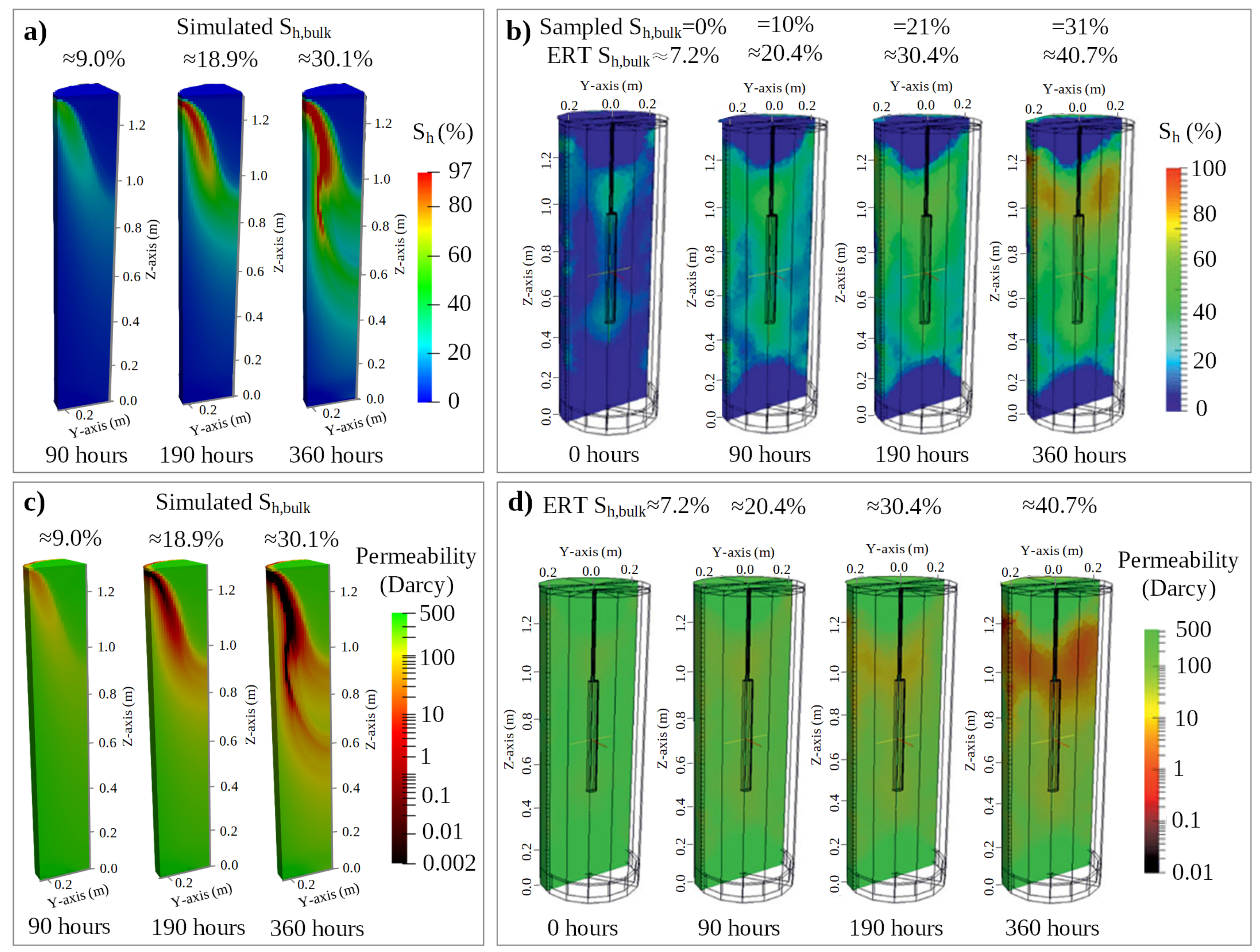
3.2.2. Model Validation by Comparison of the Temporal and Spatial Evolution of Simulated and Observed Hydrate Saturations

The evolution of spatial hydrate saturation and hydraulic permeability distributions can be described by the numerical simulations and ERT observations, separately. At hour zero of the experiment shown in Figure 7b and Figure 8b, S_h,bulk > 7.2% was determined by ERT [27]. At the end of Stage I (90 h), it is indicated by the simulation results that the majority of the formed hydrate was accumulated under the bottom of the top porous filter plate and distributed along the warm-cool fluid interface present at 1.3–0.65 m of the specimen height. Moreover, the simulated S_h,bulk reaches 9.0% (Figure 7a), showing good agreement with the pore fluid sampling data (10%), disregarding the deviation to S_h,bulk of 20.4% determined from ERT measurements (90 h in Figure 7b).

In Stage II, hydrate formation mainly occurred at 1.3–0.95 m of the specimen height, as shown for 190 h in Figure 7a,b. Furthermore, the maximum simulated S_h increased to 97% and the simulated S_h,bulk to approximately 18.9% simultaneously, which closely matches with the fluid sampling result (21%) at 190 h. Subsequently, the front of accumulated hydrate advanced to 0.95–0.65 m of specimen height, indicating a similar hydrate distribution pattern to the ERT-measured findings (cf. 360 h in Figure 7a,b). Finally, the simulated S_h,bulk increased to about 30.1%, and is thus almost identical with the corresponding S_h,bulk of 31% determined by fluid sampling at the end of Stage III. Despite the relative error of the ERT-measured S_h,bulk, it has been confirmed that hydrate initially formed at the top of the specimen, and then the front of hydrate formation advanced to the specimen center along the neoprene jacket.

In Figure 7a,b, the S_h observed by ERT and simulated are virtually zero at the bottom and top of LARS. At the top region near the inlet of LARS, the p-T conditions of the inflowing CH₄-loaded fluid are outside of the CH₄ hydrate stability range. These conditions were chosen to avoid undesired blockages by hydrate formation at the inlet. As the fluid flows through the sandy sediment sample, it cools and eventually meets the CH₄ hydrate stability conditions, whereby excess CH₄ is consumed. When the fluid flows to the bottom of the sandy sample, it is undersaturated with CH₄, so that CH₄ hydrate can no longer form despite the favoring p-T conditions.

The Carman–Kozeny Equation (A13) shows that the bulk permeability is a function of S_h,bulk, as the predefined initial permeability is constant (Table 3). Accordingly, the change in local permeability reflects the variation of S_h. At hour zero of the experiment (Figure 7d), a slightly heterogeneously distributed permeability was observed in a range of 300 to 500 Darcy. Subsequently, accumulating hydrate reduced the hydraulic permeability in the upper part of specimen. Some warmer CH₄-loaded brine advanced along the neoprene jacket, and a small amount migrated along the aforementioned buffer layer. Moreover, the electrical resistivity of the relevant region was appreciably increased [41]. On account of the constantly increasing hydrate accumulation, the permeability of the affected region was thus declining until 360 h. Finally, the minimum simulated local permeability is 2.1 mDarcy (Figure 7c) and identical to the hydraulic test results (2 mDarcy) represented by the blue dot in Figure 8a.

Overall, the simulation results confirm that ERT monitored the spatial hydrate distribution within the specimen mainly qualitatively in the early stages (before 190 h in Figure 7b) of the experiment, and the volume-averaged S_h,bulk was estimated at high precision by pore fluid sampling in previous laboratory studies [27].

3.3. Uncertainties of Critical Parameters in the Experimental Study

Initially, several essential details were collected to determine practical ranges of the input parameters (Table 4) and establish an equivalent geometrical model for calibration (Figure 4). The optimized input parameters were then determined by a history-matching procedure during model calibration, and the documented initial and boundary conditions were revised (Table 5 and Table 6). Additionally, the exact locations of RTDs could not be derived by any measurement method once the sample chamber was filled with quartz sand. Thus, these had to be revised iteratively in the present study (Table 5).

There are further uncertainties similar to those noted above. For instance, the initial intrinsic permeability of the specimen was too high and out of the measurement range of the experimental setup, thus it could exclusively be estimated empirically from porosity and grain size distribution. However, the final bulk permeability could be measured at the end of the hydrate formation experiment by a hydraulic test [27], whose result is illustrated in Figure 8a. In addition to this, the boundary condition for the inflowing fluid became time-dependent, caused by the hydrate likely forming inside the porous filter plate. Furthermore, some critical variables required for the simulation study were exclusively measured at the onset of the hydrate formation study, e.g., the external cooling and inflowing fluid temperatures as well as the dissolved CH₄ concentration in the inflowing fluid. Despite these uncertainties, most of them can be prevented or eliminated in future experimental designs by optimizing the execution of the experimental planning.

With regard to the uncertainties in the estimation of the initial permeability and S_h,bulk, the initial interpretation of Figure 8 was given in a previous study [27]. However, the remarkable differences between hydrate saturations derived from ERT measurements, conductivity measurements, and simulation are still worth noting and require further analysis. Figure 8b demonstrates that the simulation curve increases in the form of multiple steps, which is inconsistent with the simple linear growth pattern determined by pore fluid sampling and ERT measurements. It can be explained by the artificial acquisition intervals of experimental data being much larger than those in the numerical simulations. For example, the pore fluid sampling for pore fluid conductivity measurements was undertaken on a daily basis, whereas ERT measurements were only made at the end of each formation stage. Hence, these cannot characterize the detailed transition during hydrate accumulation.

Theoretically, the remarkable contrasts in electrical resistivities between the coexisting pore-filling components (pore fluid and hydrate) granted hydrate to be distinguished from the pore fluid and localized even at low S_h [27], as hydrate is electrically non-conductive. However, it should be noted that the most significant deviation of the ERT-measured S_h,bulk (ca. 7.2%) from the corresponding simulated and sampled S_h,bulk (0%) was observed at the onset of the experiment (hour zero) in Figure 8b. This is attributed to the initial assumption and relevant post-processing routine for the conversion of electrical resistivity into S_h [27]. Hereafter, the difference in hydrate content from ERT and pore fluid electrical resistivity becomes less notable as the hydrate saturation increases, particularly at S_h,bulk > 65%, when the sampled S_h,bulk finally agrees with the ERT-observed one. Eventually, the ERT-observed S_h,bulk resulted in a notable deviation of more than 10% from the corresponding sampled S_h,bulk (ca. 89%) in Figure 8b.

The ERT measurements provided useful information regarding the location where hydrate started to form and how its distribution generally changed with time, which helped to adjust the way the experiment was conducted. However, the upper and lower 0.15 m of the sample chamber are not covered with electrodes, and ERT is not able to capture effects close to the top and bottom steel closures with the fluid in- and outlets. In addition, the resolution of the ERT method is limited, and small-scale accumulations of hydrate with only little effect on electrical resistivity might not be recognized. Furthermore, the inversion process converting the resistance measurements on the sample surface into a 3D electrical resistivity distribution is not unique (as for all potential methods). The transformation of electrical resistivity into S_h relies on an empirical rock-physical model, without any specific calibration for hydrates [26,27]. This further explains the observed discrepancies to the numerical modeling.

4. Summary and Conclusions

The present study numerically reproduced a previously conducted multi-stage CH₄ hydrate formation experiment. The effectiveness and accuracy of the developed coupled numerical framework have been evaluated and demonstrated by a benchmark and comparisons to the experimental observations. Consequently, the key parameters and an optimum combination of initial and boundary conditions were determined. Our findings allow for the following conclusions:

• The general consistency of the experimental observations with the simulation results proves that the employed equilibrium CH₄ hydrate formation model can represent the main processes of hydrate formation in LARS. The equilibrium reaction model is a practicable alternative to kinetic approaches at macro-scale (vessel volume > 0.2 m³) given the application of the “dissolved-gas” method. In contrast, kinetic reaction approaches tend to be irreplaceable for modeling hydrate formation by other methods, because their CH₄ hydrate growth rates are orders of magnitude faster than that of the “dissolved-gas” method.
• The deviations among the experimental observations (i.e., continuously recorded temperature profiles, periodically gathered S_h,bulk, and ERT-tomography derived spatial S_h distributions) and the corresponding numerical predictions were minimized through an iterative optimization procedure. It has been indicated that the combination of the thermal properties of inflowing CH₄-loaded fluid and the hydrate-bearing sand determine the spatial distribution of hydrate accumulations.
• The presented spatial S_h distribution illustrates a heterogeneous accumulation within the hydrate-bearing sand at an early experimental period when S_h,bulk < 30%, with the feature becoming less prominent until S_h,bulk > 80%.
• In the LARS hydrate formation experiment, a relatively large temperature gradient (ca. 10 °C/0.23 m) is generated between the inflow of warm brine and its surrounding coolants, leading to a heterogeneous hydrate distribution. In contrast, the sub-permafrost and sub-seafloor geothermal gradients in natural settings are substantially lower (3 °C/100 m) [75] and steady for long time periods, causing a lower and almost constant dissolved CH₄ concentration gradient in the saline fluid. Therefore, relatively uniformly distributed S_h were found within the NGH intervals with ignorable lateral variations at the Mallik site. These NGH accumulation intervals could be simplified as CH₄ hydrate layers formed via the continuous supply of dissolved CH₄, migrating through the up-dip natural faults in the Canadian Beaufort-Mackenzie Basin region.

The proposed numerical framework can be utilized to improve experimental designs and optimize post-processing workflows of monitoring data. Thereby it could contribute to calibrate the advanced geophysical identification techniques and investigate dynamic hydrate accumulation processes in water-dominated geological settings at the field scale.

References

1. Kvenvolden, K.A.; Ginsburg, G.D.; Soloviev, V.A. Worldwide distribution of subaquatic gas hydrates. Geo-Mar. Lett. 1993, 13, 32–40. [Google Scholar] [CrossRef]
2. Sloan, E.D., Jr.; Koh, C.A. Clathrate Hydrates of Natural Gases, 3rd ed.; CRC Press: Boca Raton, FL, USA, 2008. [Google Scholar]
3. Yin, Z.; Moridis, G.; Tan, H.K.; Linga, P. Numerical analysis of experimental studies of methane hydrate formation in a sandy porous medium. Appl. Energy 2018, 220, 681–704. [Google Scholar] [CrossRef] [Green Version]
4. Makogon, Y.F. Natural gas hydrates—A promising source of energy. J. Nat. Gas Sci. Eng. 2010, 2, 49–59. [Google Scholar] [CrossRef]
5. Osadetz, K.G.; Dixon, J.; Dietrich, J.R.; Snowdon, L.R.; Dallimore, S.R.; Majorowicz, J.A. A Review of Mackenzie Delta-Beaufort Sea Petroleum Province Conventional and Non-Conventional (Gas Hydrate) Petroleum Reserves and Undiscovered Resources: A Contribution to the Resource Assessment of the Proposed Mackenzie Delta-Beaufort Sea Marine Protected Area. 2005. Available online: https://waves-vagues.dfo-mpo.gc.ca/Library/281345.pdf (accessed on 20 December 2021).
6. Koh, C.A.; Sum, A.K.; Sloan, E.D. Gas hydrates: Unlocking the energy from icy cages. J. Appl. Phys. 2009, 106, 061101. [Google Scholar] [CrossRef]
7. Milkov, A.V. Global estimates of hydrate-bound gas in marine sediments: How much is really out there? Earth-Sci. Rev. 2004, 66, 183–197. [Google Scholar] [CrossRef]
8. Wallmann, K.; Schicks, J.M. Gas Hydrates as an Unconventional Hydrocarbon Resource. In Hydrocarbons, Oils and Lipids: Diversity, Origin, Chemistry and Fate. (Handbook of Hydrocarbon and Lipid Microbiology); Wilkes, H., Ed.; Springer: Cham, Switzerland, 2018; pp. 1–17. [Google Scholar] [CrossRef]
9. Yin, Z.; Khurana, M.; Tan, H.K.; Linga, P. A review of gas hydrate growth kinetic models. Chem. Eng. J. 2018, 342, 9–29. [Google Scholar] [CrossRef]
10. Yin, Z.; Chong, Z.R.; Tan, H.K.; Linga, P. Review of gas hydrate dissociation kinetic models for energy recovery. J. Nat. Gas Sci. Eng. 2016, 35, 1362–1387. [Google Scholar] [CrossRef]
11. Hassanpouryouzband, A.; Joonaki, E.; Vasheghani Farahani, M.; Takeya, S.; Ruppel, C.; Yang, J.; English, N.J.; Schicks, J.M.; Edlmann, K.; Mehrabian, H.; et al. Gas hydrates in sustainable chemistry. Chem. Soc. Rev. 2020, 49, 5225–5309. [Google Scholar] [CrossRef]
12. Handa, Y.P.; Stupin, D.Y. Thermodynamic properties and dissociation characteristics of methane and propane hydrates in 70-.ANG.-radius silica gel pores. J. Phys. Chem. 1992, 96, 8599–8603. [Google Scholar] [CrossRef]
13. Winters, W.J.; Pecher, I.A.; Waite, W.F.; Mason, D.H. Physical properties and rock physics models of sediment containing natural and laboratory-formed methane gas hydrate. Am. Mineral. 2004, 89, 1221–1227. [Google Scholar] [CrossRef]
14. Priest, J.A.; Rees, E.V.L.; Clayton, C.R.I. Influence of gas hydrate morphology on the seismic velocities of sands. J. Geophys. Res. Solid Earth 2009, 114, B11205. [Google Scholar] [CrossRef] [Green Version]
15. Schicks, J.M.; Spangenberg, E.; Giese, R.; Steinhauer, B.; Klump, J.; Luzi, M. New approaches for the production of hydrocarbons from hydrate bearing sediments. Energies 2011, 4, 151–172. [Google Scholar] [CrossRef] [Green Version]
16. Fitzgerald, G.C.; Castaldi, M.J.; Zhou, Y. Large scale reactor details and results for the formation and decomposition of methane hydrates via thermal stimulation dissociation. J. Pet. Sci. 2012, 94–95, 19–27. [Google Scholar] [CrossRef]
17. Chong, Z.R.; Pujar, G.A.; Yang, M.; Linga, P. Methane hydrate formation in excess water simulating marine locations and the impact of thermal stimulation on energy recovery. Appl. Energy 2016, 177, 409–421. [Google Scholar] [CrossRef]
18. Broseta, D.; Ruffine, L.; Desmedt, A. Gas Hydrates 1: Fundamentals, Characterization and Modeling; John Wiley & Sons: Hoboken, NJ, USA, 2017. [Google Scholar]
19. Li, G.; Wu, D.; Li, X.; Zhang, Y.; Lv, Q.; Wang, Y. Experimental Investigation into the Production Behavior of Methane Hydrate under Methanol Injection in Quartz Sand. Energy Fuels 2017, 31, 5411–5418. [Google Scholar] [CrossRef]
20. Chandrasekharan Nair, V.; Mech, D.; Gupta, P.; Sangwai, J.S. Polymer flooding in artificial hydrate bearing sediments for methane gas recovery. Energy Fuels 2018, 32, 6657–6668. [Google Scholar] [CrossRef]
21. Schicks, J.M.; Strauch, B.; Heeschen, K.U.; Spangenberg, E.; Luzi-Helbing, M. From Microscale (400 μl) to Macroscale (425 L): Experimental Investigations of the CO2/N2--CH4 Exchange in Gas Hydrates Simulating the Iġnik Sikumi Field Trial. J. Geophys. Res. Solid Earth 2018, 123, 3608–3620. [Google Scholar] [CrossRef] [Green Version]
22. Thoutam, P.; Rezaei Gomari, S.; Ahmad, F.; Islam, M. Comparative analysis of hydrate nucleation for methane and carbon dioxide. Molecules 2019, 24, 1055. [Google Scholar] [CrossRef] [Green Version]
23. Pan, M.; Ismail, N.A.; Luzi-Helbing, M.; Koh, C.A.; Schicks, J.M. New Insights on a µm-Scale into the Transformation Process of CH4 Hydrates to CO2–Rich Mixed Hydrates. Energies 2020, 13, 5908. [Google Scholar] [CrossRef]
24. Schicks, J.M.; Pan, M.; Giese, R.; Poser, M.; Ismail, N.A.; Luzi-Helbing, M.; Bleisteiner, B.; Lenz, C. A new high-pressure cell for systematic in situ investigations of micro-scale processes in gas hydrates using confocal micro-Raman spectroscopy. Rev. Sci. Instrum. 2020, 91, 115103. [Google Scholar] [CrossRef]
25. Heeschen, K.U.; Deusner, C.; Spangenberg, E.; Priegnitz, M.; Kossel, E.; Strauch, B.; Bigalke, N.; Luzi-Helbing, M.; Haeckel, M.; Schicks, J.M. Production Method under Surveillance: Laboratory Pilot-Scale Simulation of CH4–CO2 Exchange in a Natural Gas Hydrate Reservoir. Energy Fuels 2021, 35, 10641–10658. [Google Scholar] [CrossRef]
26. Priegnitz, M.; Thaler, J.; Spangenberg, E.; Rücker, C.; Schicks, J.M. A cylindrical electrical resistivity tomography array for three-dimensional monitoring of hydrate formation and dissociation. Rev. Sci. Instrum. 2013, 84, 104502. [Google Scholar] [CrossRef] [PubMed]
27. Priegnitz, M.; Thaler, J.; Spangenberg, E.; Schicks, J.M.; Schrötter, J.; Abendroth, S. Characterizing electrical properties and permeability changes of hydrate bearing sediments using ERT data. Geophys. J. Int. 2015, 202, 1599–1612. [Google Scholar] [CrossRef] [Green Version]
28. Sa, J.H.; Kwak, G.H.; Han, K.; Ahn, D.; Cho, S.J.; Lee, J.D.; Lee, K.H. Inhibition of methane and natural gas hydrate formation by altering the structure of water with amino acids. Sci. Rep. 2016, 6, 31582. [Google Scholar] [CrossRef]
29. Zhang, L.; Kuang, Y.; Zhang, X.; Song, Y.; Liu, Y.; Zhao, J. Analyzing the process of gas production from methane hydrate via nitrogen injection. Ind. Eng. Chem. Res. 2017, 56, 7585–7592. [Google Scholar] [CrossRef]
30. Strauch, B.; Heeschen, K.U.; Schicks, J.M.; Spangenberg, E.; Zimmer, M. Application of tubular silicone (PDMS) membranes for gas monitoring in CO2–CH4 hydrate exchange experiments. Mar. Pet. Geol. 2020, 122, 104677. [Google Scholar] [CrossRef]
31. Heeschen, K.U.; Janocha, J.; Spangenberg, E.; Schicks, J.M.; Giese, R. The impact of ice on the tensile strength of unconsolidated sand-A model for gas hydrate-bearing sands? Mar. Pet. Geol. 2020, 122, 104607. [Google Scholar] [CrossRef]
32. Pan, M.; Schicks, J.M. Influence of Gas Supply Changes on the Formation Process of Complex Mixed Gas Hydrates. Molecules 2021, 26, 3039. [Google Scholar] [CrossRef]
33. Dai, J.; Xu, H.; Snyder, F.; Dutta, N. Detection and estimation of gas hydrates using rock physics and seismic inversion: Examples from the northern deepwater Gulf of Mexico. Lead. Edge 2004, 23, 60–66. [Google Scholar] [CrossRef] [Green Version]
34. Sell, K.; Saenger, E.H.; Falenty, A.; Chaouachi, M.; Haberthür, D.; Enzmann, F.; Kuhs, W.F.; Kersten, M. On the path to the digital rock physics of gas hydrate-bearing sediments—Processing of in situ synchrotron-tomography data. Solid Earth 2016, 7, 1243–1258. [Google Scholar] [CrossRef] [Green Version]
35. Sell, K.; Quintal, B.; Kersten, M.; Saenger, E.H. Squirt flow due to interfacial water films in hydrate bearing sediments. Solid Earth 2018, 9, 699–711. [Google Scholar] [CrossRef] [Green Version]
36. Yun, T.S.; Francisca, F.M.; Santamarina, J.C.; Ruppel, C. Compressional and shear wave velocities in uncemented sediment containing gas hydrate. Geophys. Res. Lett. 2005, 32, L10609. [Google Scholar] [CrossRef]
37. Waite, W.F.; Santamarina, J.C.; Cortes, D.D.; Dugan, B.; Espinoza, D.N.; Germaine, J.; Jang, J.; Jung, J.W.; Kneafsey, T.J.; Shin, H.; et al. Physical properties of hydrate-bearing sediments. Rev. Geophys. 2009, 47. [Google Scholar] [CrossRef]
38. Tupsakhare, S.S.; Fitzgerald, G.C.; Castaldi, M.J. Thermally Assisted Dissociation of Methane Hydrates and the Impact of CO2 Injection. Ind. Eng. Chem. Res. 2016, 55, 10465–10476. [Google Scholar] [CrossRef]
39. Schicks, J.M.; Spangenberg, E.; Giese, R.; Luzi-Helbing, M.; Priegnitz, M.; Beeskow-Strauch, B. A Counter-Current Heat-Exchange Reactor for the Thermal Stimulation of Hydrate-Bearing Sediments. Energies 2013, 6, 3002–3016. [Google Scholar] [CrossRef]
40. Heeschen, K.U.; Abendroth, S.; Priegnitz, M.; Spangenberg, E.; Thaler, J.; Schicks, J.M. Gas Production from Methane Hydrate: A Laboratory Simulation of the Multistage Depressurization Test in Mallik, Northwest Territories, Canada. Energy Fuels 2016, 30, 6210–6219. [Google Scholar] [CrossRef]
41. Spangenberg, E.; Priegnitz, M.; Heeschen, K.; Schicks, J.M. Are Laboratory-Formed Hydrate-Bearing Systems Analogous to Those in Nature? J. Chem. Eng. Data 2014, 60, 258–268. [Google Scholar] [CrossRef] [Green Version]
42. Waite, W.; Winters, W.; Mason, D. Methane hydrate formation in partially water-saturated Ottawa sand. Am. Mineral. 2004, 89, 1202–1207. [Google Scholar] [CrossRef]
43. Waite, W.; Bratton, P.M.; Mason, D.H. Laboratory formation of non-cementing, methane hydrate-bearing sands. In Proceedings of the 7th International Conference on Gas Hydrates (ICGH 2011), Edinburgh, UK, 17–21 July 2011. [Google Scholar]
44. Choi, J.H.; Dai, S.; Cha, J.H.; Seol, Y. Laboratory formation of noncementing hydrates in sandy sediments. Geochem. Geophys. Geosystems 2014, 15, 1648–1656. [Google Scholar] [CrossRef]
45. Yin, Z.; Chong, Z.R.; Hoon, K.T.; Linga, P. Effect of Multi-Stage Cooling on the Kinetic Behavior of Methane Hydrate Formation in Sandy Medium. Energy Procedia 2019, 158, 5374–5381. [Google Scholar] [CrossRef]
46. Yin, Z.; Moridis, G.; Chong, Z.R.; Linga, P. Effectiveness of multi-stage cooling processes in improving the CH4–hydrate saturation uniformity in sandy laboratory samples. Appl. Energy 2019, 250, 729–747. [Google Scholar] [CrossRef] [Green Version]
47. Kono, H.O.; Narasimhan, S.; Song, F.; Smith, D.H. Synthesis of methane gas hydrate in porous sediments and its dissociation by depressurizing. Powder Technol. 2002, 122, 239–246. [Google Scholar] [CrossRef]
48. Fitzgerald, G.C.; Castaldi, M.J.; Schicks, J.M. Methane Hydrate Formation and Thermal Based Dissociation Behavior in Silica Glass Bead Porous Media. Ind. Eng. Chem. Res. 2014, 53, 6840–6854. [Google Scholar] [CrossRef]
49. Gambelli, A.M.; Castellani, B.; Nicolini, A.; Rossi, F. Experimental study on natural gas hydrate exploitation: Optimization of methane recovery, carbon dioxide storage and deposit structure preservation. J. Pet. Sci. Eng. 2019, 177, 594–601. [Google Scholar] [CrossRef]
50. Feng, J.C.; Li, B.; Li, X.S.; Wang, Y. Effects of depressurizing rate on methane hydrate dissociation within large-scale experimental simulator. Appl. Energy 2021, 304, 117750. [Google Scholar] [CrossRef]
51. Cui, J.; Li, K.; Cheng, L.; Li, Q.; Sun, Z.; Xiao, P.; Li, X.; Chen, G.; Sun, C. Experimental investigation on the spatial differences of hydrate dissociation by depressurization in water-saturated methane hydrate reservoirs. Fuel 2021, 292, 120277. [Google Scholar] [CrossRef]
52. Spangenberg, E.; Kulenkampff, J.; Naumann, R.; Erzinger, J. Pore space hydrate formation in a glass bead sample from methane dissolved in water. Geophys. Res. Lett. 2005, 32, L24301. [Google Scholar] [CrossRef]
53. Waite, W.F.; Spangenberg, E. Gas hydrate formation rates from dissolved-phase methane in porous laboratory specimens. Geophys. Res. Lett. 2013, 40, 4310–4315. [Google Scholar] [CrossRef]
54. Berge, L.I.; Jacobsen, K.A.; Solstad, A. Measured acoustic wave velocities of R11 (CCl3F) hydrate samples with and without sand as a function of hydrate concentration. J. Geophys. Res. Solid Earth 1999, 104, 15415–15424. [Google Scholar] [CrossRef]
55. Stern, L.A.; Kirby, S.H.; Durham, W.B. Peculiarities of Methane Clathrate Hydrate Formation and Solid-State Deformation, Including Possible Superheating of Water Ice. Science 1996, 273, 1843–1848. [Google Scholar] [CrossRef]
56. Spangenberg, E.; Heeschen, K.U.; Giese, R.; Schicks, J.M. “Ester”—A new ring-shear-apparatus for hydrate-bearing sediments. Rev. Sci. Instrum. 2020, 91, 064503. [Google Scholar] [CrossRef] [PubMed]
57. Moridis, G.J. User’s Manual for the Hydrate v1.5 Option of TOUGH+ v1.5: A Code for the Simulation of System Behavior in Hydrate-Bearing Geologic Media; Technical Report; Lawrence Berkeley National Lab. (LBNL): Berkeley, CA, USA, 2014. [Google Scholar]
58. White, M.; Kneafsey, T.; Seol, Y.; Waite, W.F.; Uchida, S.; Lin, J.; Myshakin, E.; Gai, X.; Gupta, S.; Reagan, M.; et al. An international code comparison study on coupled thermal, hydrologic and geomechanical processes of natural gas hydrate-bearing sediments. Mar. Pet. Geol. 2020, 120, 104566. [Google Scholar] [CrossRef]
59. Moridis, G.J.; Kowalsky, M.B.; Pruess, K. HydrateResSim Users Manual: A Numerical Simulator for Modeling the Behavior of Hydrates in Geologic Media; Technical Report; Lawrence Berkeley National Lab.(LBNL): Berkeley, CA USA, 2005. [Google Scholar]
60. Gamwo, I.K.; Liu, Y. Mathematical Modeling and Numerical Simulation of Methane Production in a Hydrate Reservoir. Ind. Eng. Chem. Res. 2010, 49, 5231–5245. [Google Scholar] [CrossRef]
61. Zheng, R.; Li, S.; Li, X. Sensitivity analysis of hydrate dissociation front conditioned to depressurization and wellbore heating. Mar. Pet. Geol. 2018, 91, 631–638. [Google Scholar] [CrossRef]
62. Wu, C.Y.; Hsieh, B.Z. Comparisons of different simulated hydrate designs for Class-1 gas hydrate deposits. J. Nat. Gas. Sci. Eng. 2020, 77, 103225. [Google Scholar] [CrossRef]
63. Kempka, T. Verification of a Python-based TRANsport Simulation Environment for density-driven fluid flow and coupled transport of heat and chemical species. Adv. Geosci. 2020, 54, 67–77. [Google Scholar] [CrossRef]
64. Uddin, M.; Wright, F.; Dallimore, S.; Coombe, D. Gas hydrate dissociations in Mallik hydrate bearing zones A, B, and C by depressurization: Effect of salinity and hydration number in hydrate dissociation. J. Nat. Gas. Sci. Eng. 2014, 21, 40–63. [Google Scholar] [CrossRef]
65. Kowalsky, M.B.; Moridis, G.J. Comparison of kinetic and equilibrium reaction models in simulating gas hydrate behavior in porous media. Energy Convers. Manag. 2007, 48, 1850–1863. [Google Scholar] [CrossRef] [Green Version]
66. Moridis, G. Numerical Studies of Gas Production From Methane Hydrates. SPE J. 2003, 8, 359–370. [Google Scholar] [CrossRef]
67. Kashchiev, D.; Firoozabadi, A. Driving force for crystallization of gas hydrates. J. Cryst. Growth 2002, 241, 220–230. [Google Scholar] [CrossRef]
68. Malagar, B.R.; Lijith, K.; Singh, D. Formation & dissociation of methane gas hydrates in sediments: A critical review. J. Nat. Gas Sci. Eng. 2019, 65, 168–184. [Google Scholar] [CrossRef]
69. Smits, K.M.; Sakaki, T.; Limsuwat, A.; Illangasekare, T.H. Thermal conductivity of sands under varying moisture and porosity in drainage–wetting cycles. Vadose Zone J. 2010, 9, 172–180. [Google Scholar] [CrossRef]
70. Huang, D.; Fan, S.; Liang, D.; Feng, Z. Gas Hydrate Formation and Its Thermal Conductivity Measurement. Chin. J. Geophys. 2005, 48, 1201–1207. [Google Scholar] [CrossRef]
71. Gupta, A.; Lachance, J.; Sloan, E., Jr.; Koh, C.A. Measurements of methane hydrate heat of dissociation using high pressure differential scanning calorimetry. Chem. Eng. Sci. 2008, 63, 5848–5853. [Google Scholar] [CrossRef]
72. Hu, X.; Guan, J.; Wang, Y.; Keating, A.; Yang, S. Comparison of boundary and size effect models based on new developments. Eng. Fract. Mech. 2017, 175, 146–167. [Google Scholar] [CrossRef]
73. Dong, H.; Sun, J.; Lin, Z.; Fang, H.; Li, Y.; Cui, L.; Yan, W. 3D pore-type digital rock modeling of natural gas hydrate for permafrost and numerical simulation of electrical properties. J. Geophys. Eng. 2018, 15, 275–285. [Google Scholar] [CrossRef] [Green Version]
74. Wetzel, M.; Kempka, T.; Kühn, M. Diagenetic Trends of Synthetic Reservoir Sandstone Properties Assessed by Digital Rock Physics. Minerals 2021, 11, 151. [Google Scholar] [CrossRef]
75. Majorowicz, J.A.; Jones, F.W.; Judge, A.S. Deep subpermafrost thermal regime in the Mackenzie Delta basin, northern Canada—Analysis from petroleum bottom-hole temperature data. Geophysics 1990, 55, 362–371. [Google Scholar] [CrossRef]
76. Spangenberg, E. Modeling of the influence of gas hydrate content on the electrical properties of porous sediments. J. Geophys. Res. Solid Earth 2001, 106, 6535–6548. [Google Scholar] [CrossRef]
77. Kleinberg, R.L.; Flaum, C.; Griffin, D.D.; Brewer, P.G.; Malby, G.E.; Peltzer, E.T.; Yesinowski, J.P. Deep sea NMR: Methane hydrate growth habit in porous media and its relationship to hydraulic permeability, deposit accumulation, and submarine slope stability. J. Geophys. Res. Solid Earth 2003, 108. [Google Scholar] [CrossRef]
78. Delli, M.L.; Grozic, J.L. Prediction Performance of Permeability Models in Gas-Hydrate-Bearing Sands. SPE J. 2013, 18, 274–284. [Google Scholar] [CrossRef]
79. Nagashima, A. Viscosity of water substance—New international formulation and its background. J. Phys. Chem. Ref. Data 1977, 6, 1133–1166. [Google Scholar] [CrossRef] [Green Version]
80. Phillips, S.L. A Technical Databook for Geothermal Energy Utilization; Technical Report; Lawrence Berkeley National Lab. (LBNL): Berkeley, CA, USA, 1981. [Google Scholar]
81. Wagner, W.; Pruß, A. The IAPWS Formulation 1995 for the Thermodynamic Properties of Ordinary Water Substance for General and Scientific Use. J. Phys. Chem. Ref. Data 2002, 31, 387–535. [Google Scholar] [CrossRef] [Green Version]
82. Saul, A.; Wagner, W. A Fundamental Equation for Water Covering the Range from the Melting Line to 1273 K at Pressures up to 25 000 MPa. J. Phys. Chem. Ref. Data 1989, 18, 1537–1564. [Google Scholar] [CrossRef]
83. Kell, G.S. Density, thermal expansivity, and compressibility of liquid water from 0.deg. to 150.deg. Correlations and tables for atmospheric pressure and saturation reviewed and expressed on 1968 temperature scale. J. Phys. Chem. Ref. Data 1975, 20, 97–105. [Google Scholar] [CrossRef]
84. O’Sullivan, M.; Bodvarsson, G.; Pruess, K.; Blakeley, M. Fluid and Heat Flow In Gas-Rich Geothermal Reservoirs. Soc. Pet. Eng. J. 1985, 25, 215–226. [Google Scholar] [CrossRef] [Green Version]
85. Michaelides, E.E. Thermodynamic properties of geothermal fluids. Trans.-Geotherm. Resour. Counc. 1981, 5, 316–364. [Google Scholar]
86. Gudmundsson, J.S.; Thráinsson, H. Power potential of two-phase geothermal wells. Geothermics 1989, 18, 357–366. [Google Scholar] [CrossRef]
87. Kamath, V.A. Study of Heat Transfer Characteristics during Dissociation of Gas Hydrates in Porous Media. Ph.D. Thesis, University of Pittsburgh, Pittsburgh, PA, USA, 1984. [Google Scholar]
88. Battistelli, A.; Calore, C.; Pruess, K. The simulator TOUGH2/EWASG for modelling geothermal reservoirs with brines and non-condensible gas. Geothermics 1997, 26, 437–464. [Google Scholar] [CrossRef]
89. Cramer, S.D. Solubility of methane in brines from 0 to 300.degree.C. Ind. Eng. Chem. Process Des. Dev. 1984, 23, 533–538. [Google Scholar] [CrossRef]
90. Makogon, Y.F. Hydrates of Hydrocarbons; PennWell Publishing Co.: Tulsa, OK, USA, 1997. [Google Scholar]
Figure 1. Schematic of LARS setup used in the CH4 hydrate formation study (not to scale), modified from [41].
Energies 15 01974 g001
Figure 2. Temperatures observed at the installed RTDs (cf. Table 2 for their coordinates) during the hydrate formation experiment in LARS (left) with their relative location (right, not to scale). Observations at T0–T12 are modified from a hydrate formation experiment conducted by Priegnitz et al. [27].
Energies 15 01974 g002
Figure 3. (a) The 1D benchmark used for verification of the implemented numerical modelling framework (TplusH); (b) curves of CH4 solubility in water in the presence of hydrate (solid curve, derived from the equilibrium pressure) and without the presence of hydrate (dashed curve, computed by the fixed pressure) [59,60]; (c) comparison of temperature distributions along the model length, computed by TplusH and compared against those produced by HydrateResSim (HRS); (d) comparison of hydrate saturation (Sh) and CH4 concentration in fluid (CCH4) at the right boundary, computed by TplusH against those produced by HRS.
Energies 15 01974 g003
Figure 4. Simulation domain with numerical grid employed for the numerical simulations of the LARS experiment: (a) grid and inlet boundary geometry (porous filter plate at top) with cooling boundary outside the neoprene jacket; (b) model geometry of the sample chamber and cooling boundary with the outlet layer at bottom (not to scale).
Energies 15 01974 g004
Figure 5. Overview of temperature evolution during 90 h of hydrate formation: comparison of observed temperatures at the RTDs T0–T5 (a) together with T6–T9, T11, and T12, (c) with the TplusH simulation results (dashed) obtained by revising the RTD locations in the numerical model; the equilibrium line Teq identifies the CH4 hydrate stability temperature of 13.6 °C at the given pressure and salinity; (b) schematic of the revised RTD locations within LARS (not to scale). LARS T0–T12 data were adapted from the CH4 hydrate formation experiment conducted by Priegnitz et al. [27].
Energies 15 01974 g005
Figure 6. Observed and simulated temperature evolution during the 360-hour hydrate formation experiment at RTDs T0–T5 (a) together with T6–T9, T11, and T12; (b) based on the revised RTD locations (cf. Figure 5b and Table 5). LARS T0–T12 data were adapted from the CH4 hydrate formation experiment conducted by Priegnitz et al. [27].
Energies 15 01974 g006
Figure 7. Numerical model validation by: (1) comparison of the simulated hydrate saturation (Sh) distributions (a) against those measured by ERT [27] (b) at experimental times of 0, 90, 190, and 360 h; (2) comparison of the temporal evolution of simulated Sh,bulk (a) against the ERT-measured and pore fluid-sampled ones [27] (b) over selected experimental and simulation times; (3) comparison of the simulated spatial hydraulic permeability distributions (c) against ERT measurements (d) over selected experimental and simulation times, modified from Priegnitz et al. [27].
Energies 15 01974 g007
Figure 8. Observed and simulated bulk permeability alongside with the bulk hydrate saturation (Sh,bulk) evolution during the hydrate formation experiment: (a) comparison of the simulated volume-averaged permeability with the numerically inversed ERT results [27], the Carman–Kozeny relation as a function of Sh,bulk, and the bulk permeability determined by hydraulic testing (blue dot) [27] at the end of experiment [27]; (b) comparison of the simulated Sh,bulk against the sampled and ERT-measured ones, modified from Priegnitz et al. [27].
Energies 15 01974 g008