The Effect of the COVID-19 Pandemic on Traffic Flow Characteristics, Emissions Production and Fuel Consumption at a Selected Intersection in Slovakia

Abstract

The surveyof traffic intensity is used to obtain information on the number of vehicles on roads during the day. Subsequently, it is possible to derive from this the daily, weekly, and other road traffic intensity information. This survey represents the basis for the calculation of the annual average daily traffic volume and the basic characteristics of traffic flow. The COVID-19 pandemic has caused extensive economic and social damage around the world. These damages have also affected traffic. Changes in traffic behavior have mainly affected the reduction in traffic intensity on road networks. Thanks to the reduction in the demand for transport, there has also been a significant reduction in traffic delays, fuel consumption and emissions. An examination of changes in traffic intensity took place at a selected intersection in 2019, 2020 and 2021. This paper describes the effects of reducing the traffic intensity, fuel consumption and emissions obtained by microsimulation. The results obtained confirmed the reduction in traffic, which also contributed to a significant reduction in vehicle delays.

1. Introduction and Literature Review

Road transport currently encompasses a large number of vehicles. In 2020, more than 11.6 million vehicles were registered in the European Union [1]. This figure has become a serious problem, leading to road congestion, greenhouse gas emissions and fuel consumption. Therefore, traffic engineers are trying to eliminate these negative effects through research based on sustainability. Traffic flow theory is a tool that helps traffic engineers understand and express traffic flow characteristics. Millions of vehicles are on the road all the time around the world. These vehicles affect traffic flow and also interact with each other. Whether the task is to evaluate the capacity of existing roads or design new roads, most traffic engineering projects start with an assessment of traffic flow. Therefore, a traffic engineer must have a good understanding of traffic flow theory. Examining traffic flow is a very interesting and current topic [2] and it is a nonlinear dynamic phenomenon. This nonlinear behavior is most noticeable at high traffic densities. Decreasing traffic density can be affected by, e.g., reducing demand and the number of vehicles on the road network. However, vehicles are an important part of everyday life [3,4]. Nowadays, most people travel long distances almost every day. The more recent modes of transport (cars, planes, and trains) make it possible to travel long distances in an ever-decreasing time. This creates a network across the area, full of transport and communication hubs. These hubs are connected by different roads, sidewalks and highways, which are used every day by road infrastructure users for different purposes (trade, business, passenger transport, and recreation). In addition to increasing traffic volume, there is currently a problem with the increasing negative impacts of transport (pollution, greenhouse gas emissions, congestion, etc.) [5,6,7].

Reductions in the number of vehicles in the transport network can be caused by a change in traffic management, a temporary obstacle (road accident) and other restrictions. Such restrictions include the coronavirus pandemic and other pandemics, which have limited transport demand and mobility at the global level, i.e., worldwide. Changes in traffic behavior due to epidemics (e.g., the swine flu pandemic that broke out in Hong Kong in 2009) have been addressed in several studies. Liao and colleagues [8] concluded through a questionnaire-based analysis that the more the disease has spread in an area, the more people claimed to avoid public transport.

The coronavirus pandemic that occurred in early 2020 has calmed traffic down around the world [9]. This pandemic prompted governments and authorities around the world to apply significant transport and mobility restrictions. The result has been a relevant change in transport demand and traffic intensity. Huge declines in traffic intensity have been recorded worldwide [10,11,12]. The virus spread within a few months in most countries of the world, causing the traffic intensity to decline to a minimum, especially at the beginning of the pandemic.

Each country introduced measures to restrict the movement of the population to reduce the number of infected people. These measures concerned the reduction in mobility and person-to-person contact. However, it needs to be clarified that measures varied from country to country (mobility was affected differently) [13,14]. Road transport and other transport modes were gradually restricted. Schools and shops were closed, all social events and activities were cancelled, and people were forced to work from home [15]. The coronavirus had a strong impact on the daily lives of people through strict government measures restricting daily mobility [16,17,18]. As a result, people were isolated in their residences, sharply increasing their time in the home [19].

Public transport vehicles and stations were considered very risky environments for the spread of COVID-19 [20,21]. On the other hand, the number of vehicles on the road decreased, and thus emissions also decreased [22,23]. Overall, the pandemic had a huge impact on changes in mobility (e.g., decreased shared mobility, increased private mobility, etc.) [24,25].

The COVID-19 pandemic has substantially affected almost every aspect of everyday life, including traffic flow around the world, from east to west. Therefore, it is important to compare the effects of COVID-19 on traffic flow characteristics. The first studies on this topic concerned changes in traffic volumes in Wuhan [26,27]. Many publications address the reduction in different modes of transport due to COVID-19 and its impact on the whole transport system and environment. In these studies, the authors focused on examining the effects of the pandemic in Asia [28,29,30]. Another study from Poland describes an analysis of road traffic intensity in the city before and during COVID-19 restrictions [31]. In another study [32], mobile and fixed measurements of aerosol particle concentrations in ambient air in the city of Lublin during COVID-19 restrictions were performed and compared with measurements before COVID-19. In France and Italy, the pandemic reduced the traffic density by 65 to 80%, especially during peak periods [33,34]. In the United Kingdom, road traffic intensity fell by as much as 73% [35].

Comparing daily traffic volumes with the same day of the week in the same month over the past year, total domestic traffic in the United States fell by as much as 65%. As a result of this dramatic change in traffic volumes, air quality in the Los Angeles (LA) area improved significantly [36,37]. Similar statistics were provided by Google [38]. In general, country-by-country traffic volume reductions ranged from 40% to 65%.

The COVID-19 pandemic has significantly reduced urban mobility, which has been a major benefit in terms of reducing air pollution. People have started to use nonmotorized transport more, e.g., bicycles and walking [39,40].

Du et al. [36] examined the impact of COVID-19 in urban areas in their study. They used a microscopic simulation for their research and quantified the effects of traffic demand on vehicle delays, fuel consumption and emissions. Several studies describe the improvement in air quality during COVID-19 in various countries around the world. Reductions in nitrogen oxides (NOx) and particulate matter (PM) have been found in studies from China [41], India [42] and Spain [43].

Only the necessary services (groceries) and production remained in operation. Therefore, freight transport was only partially limited because it was necessary to ensure supplies [44]. Online shopping also increased, with courier companies noticing an increase in the number of consignments. These facts influenced the choice of the intersection to be examined, as many lorries pass through it. This raises a question that previously seemed impossible to answer: To what extent can reduced transport demand affect congestion, vehicle fuel consumption and produced emissions?

Further in this article, we describe:

• Materials and methods—where we describe the procedures and materials we used for our research;
• Results—we compared the basic and derived characteristics of the traffic flow and the produced emissions over 12 h according to the vehicle category;
• Discussion—a description of the achieved results and other similar studies;
• Conclusion—a summary of the whole study.

2. Materials and Methods

The main purpose of this paper was to determine changes in traffic volume, vehicle fuel consumption and emissions produced at an isolated signal-controlled intersection in Slovakia before and during COVID-19 restrictions (Figure 1). In order to find out how the coronavirus pandemic has affected road traffic intensity, it is necessary to know the intensity in the period before COVID-19 restrictions. This raises the main research question: How did the COVID-19 pandemic affect road traffic at the chosen intersection? However, this question is not given on a very specific scale and is therefore divided into several sub-questions:

How have the dependencies of road traffic characteristics changed during the pandemic?

How has the pandemic affected the production of emissions at the intersection?

The intersection is located on a road that is part of the multimodal TEN-T network, specifically the Baltic–Adriatic corridor. This intersection was chosen for our research because it represents a major traffic problem in Slovakia, which has an impact on the entire region. The transit of freight traffic passes through this intersection, which causes congestion. The biggest problem occurs on arms 2 and 4, which form the corridor and have a high intensity of vehicles and transit. Arm 1 represents the entrance to the city and also to the industrial zone, where there are several manufacturing companies. Traffic problems occur mainly during peak hours because employees travel from/to work. The traffic intensity has increased by about 10% in the last 5 years. Trucks and heavy trucks represent approximately 40% of the traffic flow, as stated by the authors of [45]. This share has increased by 8% since 2015. In our research, we recorded a share of trucks and heavy trucks of 30%. This value can be influenced by the data obtained within one working week and their average. The composition of the traffic flow is given in

Table 1. Number of vehicles in the simulation. [authors].

Year	Number of Vehicles
	All	Car	Bus	Truck	Heavy Truck
2019	23,235	17,710	851	300	4373
2020	7392	5533	234	76	1549
2021	20,987	15,861	748	225	4152

. The share of passenger cars was 3% higher over the same period [45]. During strict restrictions, many people worked from home (home office). This reduced the number of public transport passengers, but also the number of vehicles on the road network. All cultural and sporting events were cancelled, production was reduced, and restaurants and schools were also closed.

2.1. Characteristics of the Daily Traffic Intensity in 2019, 2020 and 2021

As we stated in the previous chapter, our research aimed to determine the impact of COVID-19 on traffic intensity and also environmental pollution based on the emissions produced. The distribution of road traffic during workdays usually shows certain patterns of behavior. Knowledge of the values of traffic intensity during the day and their distribution over time allows determining several measures and indicators for evaluating the traffic conditions prevailing with regard to the elements of road networks. Knowledge and understanding of changes in the distribution of traffic volume during the day are key to many aspects of traffic engineering, such as road traffic management, road safety and road traffic prognosis. The monitored indicators were compared in three periods—before the pandemic (March 2019), the first wave of the pandemic (March 2020) and the second wave of the pandemic (March 2021). We obtained traffic intensity data from the National Traffic Information Center and from the vehicle detection and traffic management system, video detection cameras and induction loops, which are part of the intelligent traffic intersection system. In Slovakia, there is the National Traffic Information System. This is a system environment that fulfils the following tasks related to the data on the actual traffic situation on the road network of Slovakia and other traffic information—acquisition, processing, provision, publication and distribution [46,47]. Specifically, we calculated and compared one average workday from 6:00 to 18:00. We calculated the value of the average workday from the working days (Monday to Friday) of one week in March for the years 2019, 2020 and 2021 (Figure 2).

As shown in Figure 2, the average traffic intensity in 2019 reached 2225 veh/h. The peak hour was not very different from other hours during the day. However, after the introduction of strict restrictions (2020), its value dropped significantly, by more than 70%, and reached 616 veh/h, as reported by the authors of [45]. In the second wave of the pandemic (2021), the average traffic intensity increased to 1736 veh/h. This increase may have been due to the restrictions in force at the beginning of 2021. The distribution of traffic intensity in individual hours for 2020 represents the minimum variability, unlike in 2019 and 2021.

2.2. Modelling Methodology and Simulation

Traffic modelling using simulation software is a good way to examine the possible impact of proposed changes. In this way, we can verify to some extent how this will affect road traffic. Of course, it is important to verify and validate the model. Then, we can compare the results to possible developments in the real world. We used Aimsun simulation software to analyze and evaluate the data. This software provides results at both the micro and macro levels. It is based on the Wiedemann and Gipps safe distance models. However, it is modified so that the individual parameters of the model are not global but are influenced by local parameters such as driver properties, geometry, the influence of vehicles in adjacent lanes, etc. The model is based on two conflicting requirements of acceleration and deceleration. The IDM model describes the dynamics of locations and speeds of individual vehicles. For a vehicle α, xα indicates its position at time t and vα its speed. Furthermore, lα indicates the length of the vehicle. To simplify the notation, we define the net distance as sα = xα-1 − lα-1, where α-1 denotes the vehicle directly in front of the vehicle α and the speed difference or approaching speed, Δvα = vα-vα-1. For a simplified version of the model, its vehicle dynamics α are then described by the following two ordinary differential equations [48]:

$${\dot{x}}_{\mathsf{\alpha }}=\frac{d{x}_{\alpha }}{dt}=v_{\mathsf{\alpha }}$$

(1a)

$${\dot{v}}_{\mathsf{\alpha }}=\frac{\mathrm{d}{v}_{\alpha }}{dt}=\mathsf{\alpha } \left(1-{\left(\frac{v_{\alpha }}{v_0}\right)}^{\delta }-{\left(\frac{s_0+v_{\alpha }T+\frac{v_{\alpha }\mathsf{\Delta }{v}_{\alpha }}{2\sqrt{ab}}}{s_{\alpha }}\right)}^2\right)$$

(1b)

where:

v₀—required speed (km/h);

s₀—minimum required net distance (m);

T—required time (s);

a—vehicle acceleration (m/s²);

b—vehicle deceleration (m/s²);

δ—exponent (-).

The simulation outputs provide values of various traffic characteristics, such as density, intensity, vehicle speed, delay time, travel time and much more. These outputs can be generated for entire road networks (intersections and road sections), either tabularly or graphically, but also as dependencies of one quantity from another [49]. The average speeds of the whole system in existing emission models are usually used to estimate emissions at the macroscopic level. Although, fuel consumption and emissions are to some extent influenced by accelerations and instantaneous vehicle speeds. This generates different emission results. Therefore, it is more appropriate to determine emissions and fuel consumption at the microscopic level and then summarize the results for the entire system [50].

Aimsun can model the instantaneous pollution emissions caused by acceleration/deceleration and speed for all vehicles in the simulation.

The Aimsun fuel consumption model assumes that every vehicle is idle, move at a constant speed, accelerates or decelerates. The condition of each vehicle is determined, and the model then calculates the fuel consumed using the appropriate equation. For decelerating and idle vehicles, the fuel consumption can be considered constant. The fuel consumption for an accelerating vehicle is given by Equation (2a) and for a moving vehicle by Equation (2b) [49]:

$$F=\left(c_1+c_{2}av\right).$$

(2a)

where:

c₁, c₂—constants (-);

a—acceleration (m/s²);

v—speed (m/s).

$$\frac{dF}{dt}=k_1\left(1+\frac{v^3}{2v_m^3}\right)+k_{2}v.$$

(2b)

where:

k₁, k₂—constants (-);

v_m—speed at which the fuel consumed per km is a minimum (m/s). Typically, this is around 50 km/h.

The QUARTET pollution emission model can model emissions for all vehicles within the simulation. As in the fuel consumption model, vehicle status (idling, constant speed, acceleration or deceleration) and vehicle speed/acceleration are used to evaluate the emissions of each vehicle for each step of the simulation.

Panis et al.’s Emission Model can model instantaneous pollutant emissions due to acceleration/deceleration and speed for all vehicles in a simulation [51]. At each step, the simulation measures emissions for each pollutant using the same equation and takes into account different values factors by vehicle type, fuel type and immediate acceleration/deceleration [49].

Each simulation step measures the emissions for each pollutant using the same equation but considering different factor values depending on the vehicle type, fuel type and immediate acceleration/deceleration. The instantaneous emissions model mainly considers carbon dioxide (CO₂), nitrogen oxides (NOx), volatile organic compounds (VOC) and particulate matter (PM). Each vehicle type involved in the simulation must have defined instantaneous emission parameters [49]. The breakdown of passenger cars by fuel type was as follows: 65% petrol, 30% diesel and 5% LPG, as stated by the authors of [52,53]. At first, we modelled the actual dimensions and design of the intersection (number of lanes on each arm) (Figure 3). Arms 1 and 3 are about 100 m long to the nearest node from the center of the intersection. Arm 2 has a length of 1300 m, and arm 4 has a length of approximately 2000 m. The importance of this length affects mainly the number of emissions produced but also the monitored variables, which apply not only to the area of the intersection but also its arms. We also set the parameters of individual vehicles—average fuel consumption, dimensions, maximum allowed speed, signal plan of the intersection and other necessary data for the simulation and the required results. The input data for the simulation represented the calculated traffic intensity (OD matrix) of the average workday.

Even before the simulation itself, it was necessary to bring the intersection model closer to reality to calibrate it. Travel time records for individual arms obtained from video recordings were used as calibration data. Calibration was verified using a GEH statistical equation, Equation (3), as described in [54,55]. There are 2 cut-off values for GEH—5.0 and 10.0. There is a good congruence between the observed and modelled hourly traffic volumes if the resulting value is less than 5.0. If the resulting value is greater than 10.0, it means there is a problem with the data or model.

$${\mathrm{GEH}}_{2021}=\sqrt{\frac{2{\left({\mathrm{M}}_{\mathrm{s}21}-{\mathrm{M}}_{21}\right)}^2}{\left({\mathrm{M}}_{\mathrm{s}21}+{\mathrm{M}}_{21}\right)}}=\sqrt{\frac{2{\left(1736.8-1748\right)}^2}{\left(1736.8+1748\right)}}=0.268=0.27.$$

(3)

where:

M_s21—simulated traffic intensity in 2021 (veh/h);

M₂₁—real traffic intensity in 2021 (veh/h).

Our calibration using the statistical formula was 0.27, which is a very good match for 2021. For 2019 and 2020, the value was 0.47 and 0.12. Based on these results, there was no need to further modify the model, as the simulated traffic intensity and real traffic intensity represented a good match in all years. Subsequently, we performed the necessary simulations, and their results are shown further in our paper.

3. Results

Based on the verification of the model, we performed a total of 50 simulations for each mentioned year. Subsequently, we compared the basic and derived characteristics of the traffic flow and the produced emissions over 12 h according to the vehicle category. The simulation output values of the compared parameters represented the average of these simulations and are given in the following section of the paper. Each parameter has a specified unit based on the simulation outputs. The following tables represent the simulation outputs for traffic characteristics (

Table 2. Resulting values of traffic parameters as simulation output.

	2019		2020		2021
Parameter	Value	Standard Deviation	Value	Standard Deviation	Value	Standard Deviation
Delay time (s/km)	256.23	16.48	12.63	0.07	80.22	27.34
Density (veh/km)	19.72	0.61	1.27	0.03	8.85	2.51
Intensity (veh/h)	1915.82	8.2	616.03	9.06	1736.8	6.28
Speed (km/h)	17.78	0.99	60.63	0.08	41.16	3.36
Stop time (s/km)	203.26	16.04	8.57	0.07	60.99	21.2
Travel time (s/km)	307.52	16.47	63.68	0.05	130.94	27.31
Number of stops (#/veh/km)	0.22	0.01	0.02	0	0.08	0.02

) and fuel consumption and pollutants (

Table 3. Resulting values of the estimated total fuel consumption and emissions produced for the whole simulation.

		Emissions
Year	Fuel Consumption	CO2		NOx		PM		VOC
	(L)	(kg)	(kg/km)	(kg)	(kg/km)	(kg)	(kg/km)	(kg)	(kg/km)
2019	12,883	62,974.6	3540.7	658.8	37.4	16.3	0.92	51.8	2.9
2020	2102	4564.7	256.7	33.9	1.9	0.52	0.03	4.6	0.26
2021	7778	34,868.8	1960.5	361.8	20.3	7.47	0.42	29.7	1.67

).

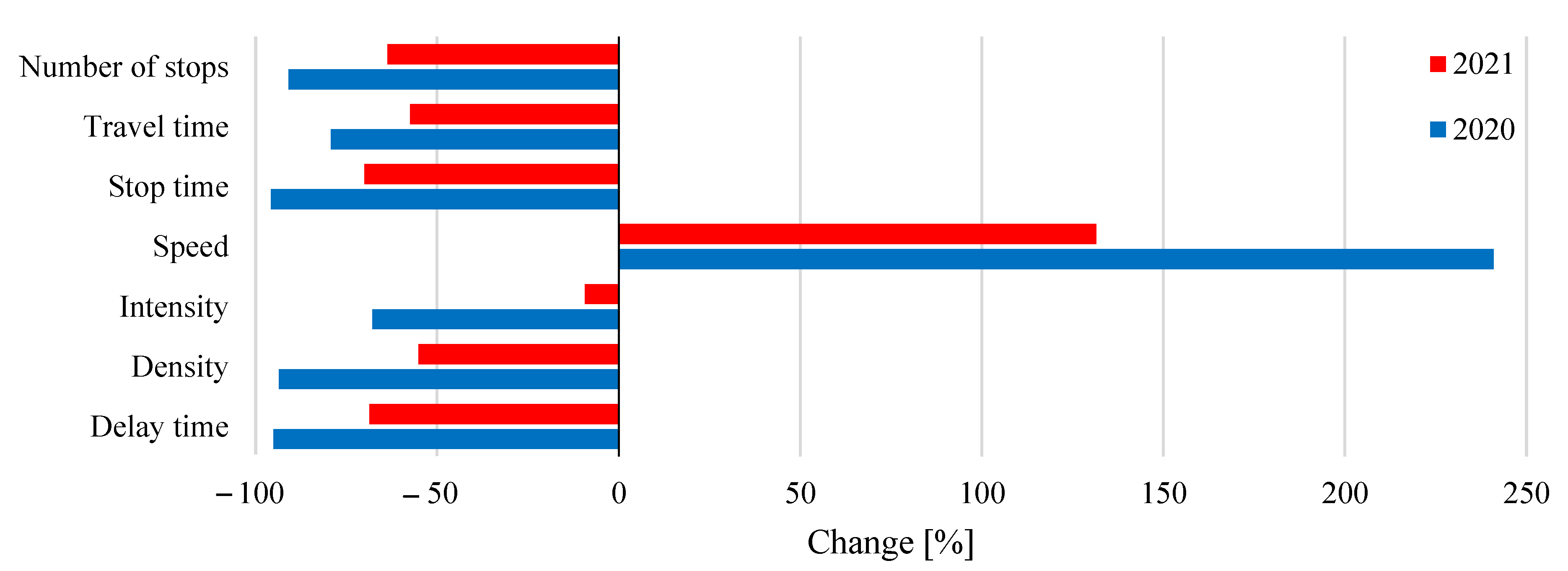
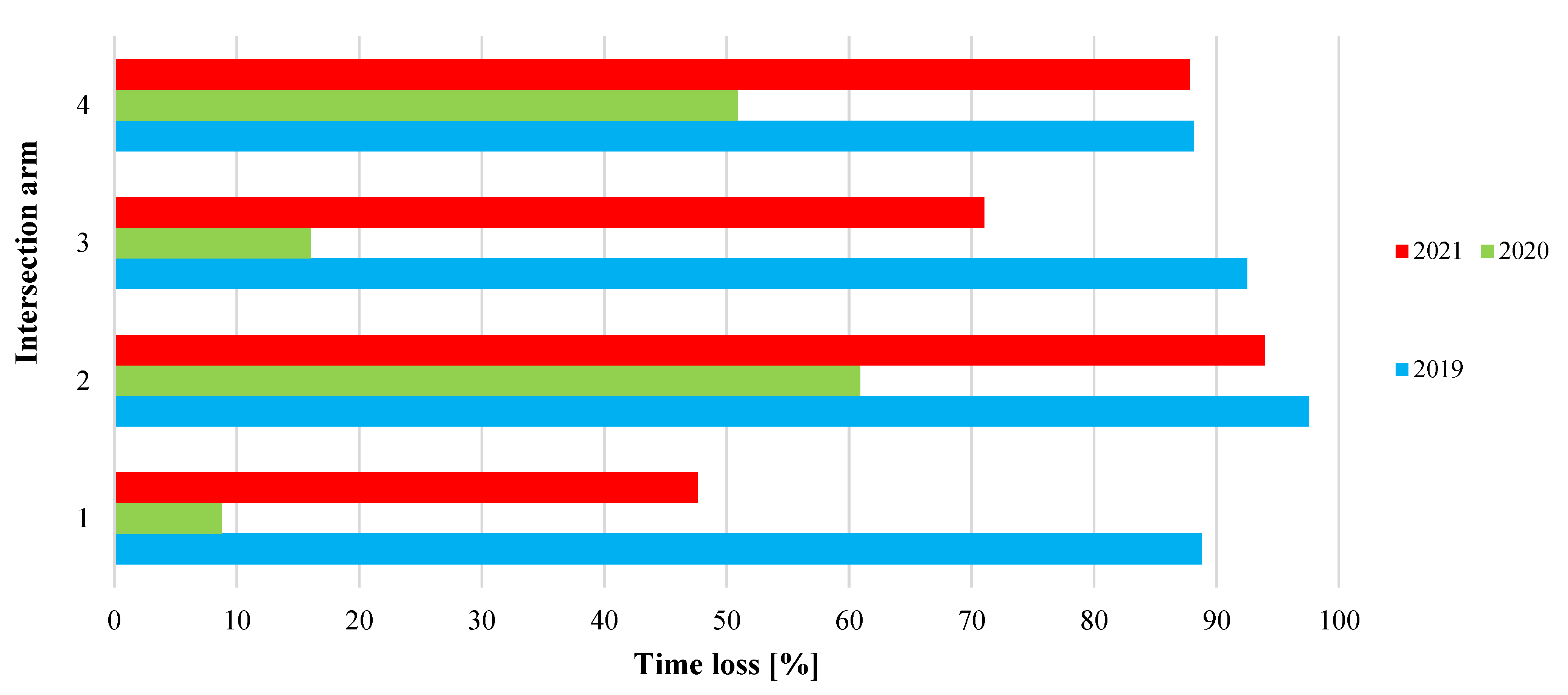
3.1. Traffic Parameters

Table 2 shows the values of traffic parameters as the output of the simulation in 2019, 2020 and 2021 at the intersection.

The highest values of traffic intensity, density, travel time, delay time and the lowest average speed of vehicles at the intersection occurred in 2019. After the introduction of restrictions related to COVID-19, the traffic intensity decreased by almost 70% (2020). On the other hand, the highest average speed was found in 2020, which increased by approximately 241%. Other parameters decreased on average between 79 and 96% compared to 2019. The highest decrease was recorded for the delay time and stop time. In 2021 (compared to 2019), there was a positive change in the decline of the monitored parameters between 9% and 70% (speed increased by almost 132%). Even in this case, the highest decrease was achieved by the delay time and travel time. The introduction of restrictions against the spread of COVID-19 had a positive effect on the traffic situation at the intersection. The percentage change was graphically processed from the monitored parameters and is shown in Figure 4.

The zero axis represents the values of 2019 and reflects the change due to pandemic restrictions. The highest increase was in the speed of vehicles due to the decrease in average traffic intensity. The vehicles passed the intersection smoothly without stopping. At the same time, the number of stops at the intersection decreased, which led to a lower production of pollutants.

After evaluating the changes in traffic at the intersection due to COVID-19 restrictions, we made a comparison between the vehicle categories. As bicycles and motorcycles accounted for only 1% of the total traffic, they were excluded from this analysis. We examined changes for passenger cars, trucks, buses and heavy trucks.

Figure 5 shows the changes in the dependences of the basic characteristics of the traffic flow. The fundamental diagram (FD) describes a well-defined equation curve for traffic flow speeds and density in steady-state traffic. The traffic flow model is based on the utilization of the continuity equation for the flow of an ideal fluid. The principles of fluid dynamics are then used to derive the equations between the basic characteristics of the traffic flow (speed, density, and intensity). The continuity equation and the equation of state (speed density and intensity density) are the basic equations of traffic flow [56]:

$$M=D·v.$$

(4)

where:

M—intensity (veh/h);

D—density (veh/km);

v—speed (km/h).

Using the equation that defines M, D and s at a given point x and time t, we can evaluate the system by measuring such delays, travel time, etc. The assumption is that vehicles flow from left to right, and the continuity equation can be written as:

$$\frac{\partial D\left(x, t\right)}{\partial t}+\frac{\partial M\left(x, t\right)}{\partial x}=0$$

(5)

FD is crucial for the study of characteristics and dynamics of traffic flow in various spatial scales using methods of analysis, modelling and simulation [56]. We created FDs for each mentioned year and compared them. The results represent an average hour from the simulation.

A decrease in traffic intensity is a predictor of a higher traffic speed and a lower density. Thus, according to theoretical estimates, a linear relationship between these characteristics is expected. In 2019, the density was approximately 20 veh/h at a speed of 17 km/h. The speed values were from 15 to 42 km/h and the density from 8 to 25 veh/h. With this variance, the linear relationship is well visible as in 2021. However, in this case, the speed variance is 17 km/h, and the density has reached a variance of 7.5 veh/h. Speed and density variance values decreased by 37% and 56% compared to 2019. However, in 2020, after the introduction of pandemic restrictions, the speed variance was only 4 km/h, and the density was only 0.3 veh/h. This fact is also related to the other two dependencies. As the intensity decreased, the speed increased and the density decreased. The rapid increase in the intensity caused traffic congestion, which is currently a major problem. Figure 6 shows the change in terms of decreases/increases in simulated characteristics depending on individual vehicle categories. The most significant decrease in average intensity was recorded for buses in both years. This fact could be due to a high decrease in demand for public transport. The delay time decreased for all vehicle categories by more than 69% in 2020 and 2021.

The delay time is the most important parameter in terms of traffic quality. Travel time is one of the largest categories of transport costs, and saving time is often considered to be the largest benefit in transport projects such as road improvements and public transport [57]. Therefore, in the following section, we focus on the analysis of time loss.

From the travel time and delay time, the time loss was determined for the entire intersection, but also for individual arms. The delay time for each vehicle category is given in the Annex. Saving travel time is one of the effects not appreciated by the market, which plays an important role in projects in the transport sector. The time loss was determined as the ratio between the average travel time and the delay time in each direction and describes the quality of traffic in the monitored section. The time loss for 2019 was almost 83.5%. In 2020, its value decreased significantly to 19.8%, but in 2021 it increased again to 61.3%.

Figure 7 shows the differences between the time loss in each year for individual arms. The highest time loss was recorded for arm 2, where the highest share of vehicles was (2019), and on arm 3, where vehicles use only one lane for all directions. This means that the vehicles limit each other, and congestion is formed, reaching as far as the city. Vehicles waiting to pass through an intersection produce higher emissions by constantly decelerating and accelerating. In Slovakia, the state of the epidemic began in mid-March 2020. The introduction of restrictions closed schools, and many people worked from home. Hence, the share of cars at the intersection decreased. Thus, it is possible to see a significant decrease in time loss for individual arms (green color). The highest decrease was for arms 1 and 3 for both years (2020 and 2021). This decrease was mainly due to the reduction in the number of cars, as these arms lead to residential areas. On the other hand, a high number of trucks were found on arms 2 and 4. Therefore, the decrease in time loss for these arms is not so significant and reached a value of 37 and 38% less than in 2019. Although restrictions affecting mobility were in force in 2021, the time loss approached the values of 2019 (arms 2 and 4).

3.2. Emissions Produced

In the transport sector and other sectors where fossil fuels are used, there is local air pollution with harmful gases. During the COVID-19 pandemic, transport demand decreased, resulting in a significant reduction not only in traffic delays, but also in energy consumption and emissions production. The Aimsun fuel consumption model assumes that each vehicle is either idle, at a constant speed, accelerating or decelerating. The condition of each vehicle is determined, and the model then calculates the fuel consumed for that condition using the appropriate formula.

Another important assessment relates to fuel consumption and air pollution. The estimation of the mentioned parameters results from the outputs of the entire length of the simulation (12 h). After the introduction of the measures (2020 and 2021), the traffic intensity decreased significantly, and the vehicles had the lowest number of stops and smoother driving (their acceleration was minimal), which reflects the average speed at the intersection. Table 3 summarizes the estimated production of emissions and fuel consumption as a simulation output.

Table 3 shows that the restrictions had a positive effect on the production of pollutants. By reducing traffic intensity, fuel consumption fell by more than 83% in 2020. By 2021, a decrease in consumption of 50% was recorded. Thus, when recalculated per vehicle, the average consumption for 2019 was estimated at 0.55 L. In 2020, this value decreased to 0.28 L (−49%), and in 2021 it reached 0.37 L (−32.7%). The following

Table 4. Estimation of emissions produced by vehicles during the simulation.

Emission	Type Vehicle	2019	2020	Change (%)	2021	Change (%)
CO2	All	62,974.6	4564.7	−92.8	34,868.8	−44.6
	Car	45,623.1	2027.0	−95.6	25,346.9	−44.4
	Truck	2209.6	233.8	−89.4	361.4	−83.6
	Bus	118.9	63.5	−46.5	218.4	83.7
	Heavy truck	15,023.1	2240.3	−85.1	8942.2	−40.5
NOX	All	658.9	33.9	−94.9	361.8	−45.1
	Car	467.8	5.9	−98.7	259.0	−44.6
	Truck	24.2	2.6	−89.4	1.2	−95.2
	Bus	2.3	0.6	−71.9	0.6	−75.4
	Heavy truck	166.3	24.8	−85.1	99.4	−40.2
PM	All	16.3	0.5	−96.8	7.5	−54.2
	Car	12.2	0.3	−97.4	5.8	−52.5
	Truck	0.6	0.0	−95.5	0.1	−82.1
	Bus	0.1	0.0	−88.4	0.0	−49.2
	Heavy truck	3.5	0.2	−94.9	1.5	−55.6

represents % changes of emission production between individual years for all vehicle categories.

Although passenger cars make up the bulk of the traffic flow, trucks achieved a higher fuel consumption (Figure 8). This could be due to the length of the arms, which could also be factored into calculations of fuel consumption and emissions. The following Figure 8 describes the estimated fuel consumption for each vehicle category.

In 2019 and 2021, the total fuel consumption during the simulation increased for all vehicle categories. In both cases, this increase could be due to the higher traffic intensity of randomly entering vehicles. The highest fuel consumption was achieved by heavy trucks in all three simulated years. On the contrary, in 2020, the total fuel consumption of vehicles was around 30 L. The fuel consumption of heavy trucks in this year differed by 35% from passenger cars. In 2019 and 2021, the differences in fuel consumption between heavy trucks and passenger cars were 15% and 25%. This difference could be due to a larger number of cars, in contrast to 2020, when this number decreased as a result of the restrictions. The total number of vehicles entering the simulation is given in the Annex. In addition to this, the distance travelled by the vehicles during the simulation is also important. In 2019, vehicles drove a total of 50,204 km for a 12 h simulation of the intersection. The average fuel consumption reached 0.55 L per vehicle. In 2020, the average fuel consumption was 0.12 L per vehicle, and the total length travelled by vehicles was 16,593 km. In 2021, fuel consumption was 0.16 L per vehicle, and vehicles travelled a total of 47,065 km.

In addition to the total fuel consumption, we compared the estimated emissions production in kg for individual vehicle categories—Figure 9, Figure 10 and Figure 11.

We compared the three emissions produced—CO₂, NOx and PM. The main human activity that releases CO₂ is the burning of fossil fuels (coal, natural gas and oil) for energy and transport purposes. Nitrogen oxides (NOx) are also formed when fuel is burned at high temperatures. In transport, the burning of fossil fuels for the transport of people and goods in 2019 was the largest source of CO₂ emissions [58]. The pollutant CO₂ contributes to the creation of greenhouse gas emissions, leading to global warming. The last evaluated emission was particulate matter. Most PM is formed in the atmosphere due to the complex reactions of chemicals such as sulfur dioxide and nitrogen oxides, which are pollutants emitted by cars. The particles contain microscopic solids or droplets of liquid that are so small that they can be inhaled and cause serious health problems. The smaller the particles, the more dangerous they are. Soot is also one of these extremely dangerous particles. They arise from imperfect carbon combustion, e.g., in diesel engines. Delay time values for all vehicle categories in individual years are in the following Figure 12, Figure 13 and Figure 14.

The graphical comparison of the produced emissions shows the decrease in the emission estimate (see simulation outputs). In 2019, the capacity of the intersection was overloaded. This caused an increased number of stops and had a negative impact on the emissions produced. By reducing the number of vehicles in 2020, especially cars, the value of CO₂ decreased by 92% compared to 2019. Trucks reduced CO₂ production by more than 85%.

With the recovery of the economy and the growth in energy consumption, emissions began to rise in 2021. The intensity of all vehicles climbed to 75% of the traffic volume from 2019. On the other hand, the decrease in CO₂ did not only reach 25% but up to 44.6%.

Traffic at the intersection became smoother as the time of delay of vehicles reduced. Thus, the vehicles showed a much smaller number of accelerations and decelerations. The number of stops per vehicle decreased by 10 times. This fact can also be seen between 2019 and 2021. There was no significant difference in the number of heavy trucks. However, NOx production decreased by more than 45% and by 40% for heavy trucks. Although, the difference in the number of vehicles was only 5%. For 2020, this decrease was almost 95% and reached its lowest value for cars (98%). The reason was the high decrease in the number of cars due to work from home and the closure of schools. The NOx values in the observed period in 2020 in Slovakia decreased by more than 27% compared to 2019 [45].

The positive impact of the restrictions on the quality of traffic at the intersection is due to the increased fluidity of the traffic flow (lower intensity and higher vehicle speed). In addition, it can be observed that the strict restrictions adopted have also been beneficial for humans—with the advantages of clean air. As in previous cases, PM values fell by almost 98% in 2020 and by 54% in 2021. However, in 2020 the highest decrease was recorded by passenger cars—97.4%. However, in 2021, heavy trucks achieved the highest decline, 3% lower than passenger cars.

These simulation results show that by reducing the traffic intensity, it is possible to increase the traffic flow at intersections. This leads to a reduction in the delay time and stop time of the vehicles. Additionally, it is possible to reduce emissions in this way. These parameters have fallen the most—by more than 81%. The impact on delay time is the most significant result of changes in demand. A decrease in the traffic intensity by 68% (2020) brought about a decrease in fuel consumption by 83.6% and a decrease in emissions by 88%. In the case of the decrease in traffic intensity of less than 10% (year 2021), fuel consumption decreased by 39.6%, and emissions by more than 48%. These results are reflected from several factors, e.g., the composition of the traffic flow, its speed, etc.

4. Discussion

The results of this research show that reducing transport demand is a very effective method to reduce traffic congestion and air pollution. For example, lifestyle changes, the increasing dependence on e-commerce, and the home office have reduced unnecessary travel [59]. The social distance initiatives adopted by most governments have yielded some positive results for the global climate. Not all of these changes have a positive impact on greenhouse gas emissions and other aspects of sustainability. According to several studies [31,60,61,62], the largest decrease in traffic intensity occurred in 2020 during the first wave of the pandemic. The authors of previous studies [31,60,61,62] report up to a 65% reduction in traffic intensity in France and Spain. In Greece, traffic intensity fell by more than 80% during the most severe period of the pandemic [63], and the US reported a decrease of almost 48% [64]. In our study, we recorded a reduction in the traffic intensity of more than 68%. In 2021, traffic intensity did not reach such a significant decrease. It decreased by an average of 35% compared to 2019. An international research team stated an extraordinary decrease in CO₂ emissions (8.8%) compared to 2019 in the same period [40]. In a study from the USA [65], there was a significant reduction in traffic intensity (71% fewer cars and 46% fewer trucks) during the restrictions and lockdown.

The estimate of fuel consumption showed decreases of more than 83% (2020) and 40% (2021) due to the pandemic in our study. Vehicle emissions (CO₂, NOx, PM) at the intersection fell by 88.4% and 48.6% on average. The estimate of fuel consumption and produced emissions would be more accurate if we also had data on the shares of individual emission limits in the traffic flow.

Nevertheless, it is not possible to say with certainty that this pandemic will permanently affect climate change. In terms of the production of emissions, studies do not indicate how long it will take to reduce them due to the economic damage caused by the pandemic [66]. On the other hand, there are efforts being made to reduce CO₂ emissions in other ways than the current impact of the pandemic. There are many alternative ways to reduce the negative effects of transport on the environment and human health. The authors of the study [67] focused on CO₂ reduction through liquefied natural gas (LNG) vehicles, and the authors of the study [68] focused on LPG vehicles from economic, emissions production and safety perspectives. This can be important for trucks but also for public transport. The pandemic has had a very negative effect on public transport. Public transport demand significantly decreased, and people have begun to prefer individual car transport, especially for fear of possible contagion. The risk of contagion can be very high due to the length of the trip and other characteristics during the trip. Therefore, studies have been carried out focusing on proposals for preventive and control restrictions for public transport facilities [69,70]. Some research predicts a steady decrease in demand for public transport due to the pandemic [4,71,72]. People’s daily mobility has been disrupted, and this has affected their travel habits. Various studies have shown a significant reduction in travel time, as well as travelled distance [73], but also a change in the mode of transport, especially public transport [74,75]. Further research is needed to determine the long-term effects of a pandemic.

The systematic analysis we conducted makes it possible to obtain typical characteristics of transport variability during the day, and can be used to create and manage transport models. The restrictions were reflected in the transport demand and pointed to changes in mobility. Further research is needed into new transport demand models able to understand the changed scenario (home office and online learning). Transport policymakers should also consider the advantages and disadvantages of this scenario in the future. How could a positive change (reduction in negative effects on the environment resulting from a decrease in traffic volume) manifest itself in a negative expression, e.g., on the psyche of the people.

5. Conclusions

Our study aimed to determine the impact of COVID-19 restrictions on the traffic situation at a signal-controlled intersection. We compared the same period (average working day in March) in the years 2019, 2020 and 2021. Continuous measurement of the traffic situation allows for the creation of a comprehensive picture and analysis of traffic fluctuations during the day, week, or another time period. We obtained the data from the National Traffic Information Center and by video detection at the intersection. Several simulations were performed in Aimsun to verify the impact of the COVID-19 restrictions on road traffic. In addition to changes in the basic characteristics of the traffic flow, we also recorded changes in fuel consumption and the production of emissions. The findings suggest that reducing the number of vehicles on the road is a very effective tool. The results showed that the mobility of the population decreased sharply because of the restrictions, which caused a significant decrease in the number of vehicles at the intersection. This reduction represented an almost 70% decrease in 2020. The following year (2021), the decrease in intensity was not so significant. The results of this paper also show that reducing transport demand is a very effective way to reduce congestion and air pollution. In any case, it is possible to observe changes in the traffic situation at the intersection, which affected the daily intensity of vehicles. The decrease in the number of vehicles represents a positive change for society in the form of reduced noise and vibration, but also lower amounts of emissions produced as vehicles pass smoothly through the intersection.

Several studies have described the impact of the pandemic and the state of emergency with regard to all modes of transport in the world. The demand for transport has fallen sharply as a result of the pandemic. Transport policymakers should therefore consider reducing post-pandemic transport demand by increasing the share of the home office, carsharing, the use of public transport, or the use of new technologies. On the one hand, such changes in travel could have significant benefits for the transport system. We would like to focus further research on changing the type of intersection. How this change will affect vehicles delay times, fuel consumption and emissions. In addition, we want to examine how people’s behavior in choosing a vehicle has changed in connection with the COVID-19 pandemic. We expect an increased interest in reducing emissions. Likewise, we would like to point out the need to build a bypass (near this locality) and its impact on the production of emissions and the diversion of transit traffic.

On the other hand, we cannot expect people to travel less and not use their vehicles right after the pandemic has ended. This change will only occur over a longer time. Measures and restrictions to motivate people to travel by public transport or shared mobility services play an important role. We believe that maintaining lower demand and reducing traffic intensity will bring sustainable environmental benefits.

References

1. ACEA: Motor Vehicle Registrations in The Eu, by Country and per Vehicle Type. Available online: https://www.acea.auto/figure/motor-vehicle-registrations-in-eu-by-country-and-per-vehicle-type/ (accessed on 21 December 2021).
2. Ou, H.; Tang, T.-Q. Impacts of moving bottlenecks on traffic flow. Phys. A Stat. Mech. Its Appl. 2018, 500, 131–138. [Google Scholar] [CrossRef]
3. Regragui, Y.; Moussa, N. Investigating the impact of real-time path planning on reducing vehicles traveling time. In Proceedings of the 2018 International Conference on Advanced Communication Technologies and Networking (CommNet), Marrakech, Morocco, 2–4 April 2018. [Google Scholar]
4. Borkowski, P.; Jażdżewska-Gutta, M.; Szmelter-Jarosz, A. Lockdowned: Everyday mobility changes in response to COVID-19. J. Transp. Geogr. 2020, 90, 102906. [Google Scholar] [CrossRef]
5. Simoni, M.D.; Marcucci, E.; Gatta, V.; Claudel, C.G. Potential last-mile impacts of crowdshipping services: A simulation-based evaluation. Transportation 2020, 47, 1933–1954. [Google Scholar] [CrossRef]
6. Afrin, T.; Yodo, N. A Survey of Road Traffic Congestion Measures towards a Sustainable and Resilient Transportation System. Sustainability 2020, 12, 4660. [Google Scholar] [CrossRef]
7. Cződörová, R.; Dočkalik, M.; Gnap, J. Impact of COVID-19 on bus and urban public transport in SR. Transp. Res. Procedia 2021, 55, 418–425. [Google Scholar] [CrossRef]
8. Liao, Q.; Cowling, B.J.; Wu, P.; Leung, G.M.; Fielding, R.; Lam, W.W.T. Population Behavior Patterns in Response to the Risk of Influenza A(H7N9) in Hong Kong, December 2013–February 2014. Int. J. Behav. Med. 2015, 22, 672–682. [Google Scholar] [CrossRef] [PubMed]
9. Lum, L.H.W.; Tambyah, P.A. Outbreak of COVID-19—An urgent need for good science to silence our fears? Singap. Med. J. 2020, 61, 55–57. [Google Scholar] [CrossRef] [PubMed]
10. Kraemer, M.U.G.; Chia-Hung, Y.; Bernardo, G.; Chieh-Hsi, W.; Brennan, K.; David, M.P. The effect of human mobility and control measures on the COVID 19 epidemic in China. Science 2020, 368, 493–497. [Google Scholar] [CrossRef] [PubMed] [Green Version]
11. Cui, Z.; Meixin, Z.; Shuo, W.; Pengfei, W.; Yang, Z.; Qianxia, C.; Cole, K.; Yinhai, W. Traffic performance score for measuring the impact of COVID-19 on urban mobility. arXiv 2020, arXiv:2007.00648. [Google Scholar]
12. Heiler, G.; Tobias, R.; Jan, H.; Mohammad, F.; Aida, O.; Allan, H.; Farid, K. Country-wide mobility changes observed using mobile phone data during COVID-19 pandemic. arXiv 2020, arXiv:2008.10064. [Google Scholar]
13. Alipour, J.-V.; Fadinger, H.; Schymik, J. My home is my castle—The benefits of working from home during a pandemic crisis. J. Public Econ. 2021, 196, 104373. [Google Scholar] [CrossRef]
14. Askitas, N.; Tatsiramos, K.; Verheyden, B. Lockdown Strategies, Mobility Patterns and COVID-19. IZA Discussion Papers 2020; Institute of Labor Economics (IZA): Bonn, Germany, 2020; p. 13293. [Google Scholar]
15. Epstein, J.M.; Goedecke, D.M.; Yu, F.; Morris, R.J.; Wagener, D.K.; Bobashev, G.V. Controlling Pandemic Flu: The Value of International Air Travel Restrictions. PLoS ONE 2007, 2, e401. [Google Scholar] [CrossRef] [PubMed]
16. Bönisch, S.; Wegscheider, K.; Krause, L.; Sehner, S.; Wiegel, S.; Zapf, A.; Moser, S.; Becher, H. Effects of Coronavirus Disease (COVID-19) Related Contact Restrictions in Germany, March to May 2020, on the Mobility and Relation to Infection Patterns. Front. Public Health 2020, 8, 568287. [Google Scholar] [CrossRef]
17. Hsiehchen, D.; Espinoza, M.; Slovic, P. Political partisanship and mobility restriction during the COVID-19 pandemic. Public Health 2020, 187, 111–114. [Google Scholar] [CrossRef] [PubMed]
18. Bonaccorsi, G.; Pierri, F.; Cinelli, M.; Flori, A.; Galeazzi, A.; Porcelli, F.; Schmidt, A.L.; Valensise, C.M.; Scala, A.; Quattrociocchi, W.; et al. Economic and social consequences of human mobility restrictions under COVID-19. Proc. Natl. Acad. Sci. USA 2020, 117, 15530–15535. [Google Scholar] [CrossRef]
19. Fukumoto, K.; McClean, C.T.; Nakagawa, K. No causal effect of school closures in Japan on the spread of COVID-19 in spring 2020. Nat. Med. 2021, 27, 2111–2119. [Google Scholar] [CrossRef]
20. Musselwhite, C.; Avineri, E.; Susilo, Y. Editorial JTH 16 –The Coronavirus Disease COVID-19 and implications for transport and health. J. Transp. Health 2020, 16, 100853. [Google Scholar] [CrossRef] [PubMed]
21. Des Transport Publics, Union Internationale. Management of COVID-19 Guidelines for Public Transport Operators. Available online: https://www.uitp.org/publications/management-of-covid-19-guidelines-for-public-transport-operators/ (accessed on 22 December 2020).
22. Caraka, R.; Lee, Y.; Kurniawan, R.; Herliansyah, R.; Kaban, P.; Nasution, B.; Gio, P.; Chen, R.; Toharudin, T.; Pardamean, B. Impact of COVID-19 large scale restriction on environment and economy in Indonesia. Glob. J. Environ. Sci. Manag. 2020, 6, 65–84. [Google Scholar] [CrossRef]
23. Huang, X.; Ding, A.; Gao, J.; Zheng, B.; Zhou, D.; Qi, X.; Tang, R.; Wang, J.; Ren, C.; Nie, W.; et al. Enhanced secondary pollution offset reduction of primary emissions during COVID-19 lockdown in China. Natl. Sci. Rev. 2021, 8, 1–9. [Google Scholar] [CrossRef]
24. Pawar, D.S.; Yadav, A.K.; Akolekar, N.; Velaga, N.R. Impact of physical distancing due to novel coronavirus (SARS-CoV-2) on daily travel for work during transition to lockdown. Transp. Res. Interdiscip. Perspect. 2020, 7, 100203. [Google Scholar] [CrossRef] [PubMed]
25. Deponte, D.; Fossa, G.; Gorrini, A. Shaping space for ever-changing mobility. COVID-19 lesson learned from Milan and its region. TeMA J. Land Use Mobil. Environ. J. Land Use Mobil. Environ. 2020, 133–149. [Google Scholar] [CrossRef]
26. Tanveer, H.; Balz, T.; Cigna, F.; Tapete, D. Monitoring 2011–2020 Traffic Patterns in Wuhan (China) with COSMO-SkyMed SAR, Amidst the 7th CISM Military World Games and COVID-19 Outbreak. Remote Sens. 2020, 12, 1636. [Google Scholar] [CrossRef]
27. Shi, Z.; Fang, Y. Temporal relationship putbound traffic from Wuhan and the 2019 coronavirus disease (COVID-19) incidence in China. MedRxiv 2020. [Google Scholar] [CrossRef] [Green Version]
28. Lai, I.-C.; Brimblecombe, P. Long-range Transport of Air Pollutants to Taiwan during the COVID-19 Lockdown in Hubei Province. Aerosol Air Qual. Res. 2021, 21, 200392. [Google Scholar] [CrossRef]
29. Kanniah, K.D.; Zaman, N.A.F.K.; Kaskaoutis, D.G.; Latif, M.T. COVID-19’s impact on the atmospheric environment in the Southeast Asia region. Sci. Total Environ. 2020, 736, 139658. [Google Scholar] [CrossRef] [PubMed]
30. Şahin, A. The Effects of COVID-19 Measures on Air Pollutant Concentrations at Urban and Traffic Sites in Istanbul. Aerosol Air Qual. Res. 2020, 20, 1874–1885. [Google Scholar] [CrossRef]
31. Macioszek, E.; Kurek, A. Extracting Road Traffic Volume in the City before and during COVID-19 through Video Remote Sensing. Remote Sens. 2021, 13, 2329. [Google Scholar] [CrossRef]
32. Polednik, B. COVID-19 lockdown and particle exposure of road users. J. Transp. Health 2021, 22, 101233. [Google Scholar] [CrossRef] [PubMed]
33. Pullano, G.; Valdano, E.; Scarpa, N.; Rubrichi, S.; Colizza, V. Population mobility reductions during COVID-19 epidemic in France under lockdown. medRxiv 2020. [Google Scholar] [CrossRef]
34. Ravina, M.; Esfandabadi, Z.S.; Panepinto, D.; Zanetti, M. Traffic-induced atmospheric pollution during the COVID-19 lockdown: Dispersion modeling based on traffic flow monitoring in Turin, Italy. J. Clean. Prod. 2021, 317, 128425. [Google Scholar] [CrossRef] [PubMed]
35. Carrington, D. UK Road Travel Falls to 1955 Levels as COVID-19 Lockdown Takes Hold. The Guardian, (3 April 2020). Available online: https://www.theguardian.com/uk-news/2020/apr/03/uk-road-travel-falls-to-1955-levels-as-covid-19-lockdown-takes-hold-coronavirus-traffic (accessed on 20 November 2021).
36. Du, J.; Rakha, H.A.; Filali, F.; Eldardiry, H. COVID-19 pandemic impacts on traffic system delay, fuel consumption and emissions. Int. J. Transp. Sci. Technol. 2020, 10, 184–196. [Google Scholar] [CrossRef]
37. Mendoza, D.L.; Benney, T.M.; Ganguli, R.; Pothina, R.; Krick, B.; Pirozzi, C.S.; Crosman, E.T.; Zhang, Y. Understanding the relationship between social distancing policies, traffic volume, air quality, and the prevellence of COVID-19 outcomes in urban neighborhoods. Phys. Soc. 2020, 1–34. [Google Scholar] [CrossRef]
38. Google, 2020. Commnuity Mobility Report. Available online: https://www.google.com/covid19/mobility/?fbclid=IwAR1nnjn3vNyO4qcnMtkcZBN6FVuL1tpFL-NtI4_nKkfVHU-gaM_OhrG9U1w (accessed on 21 November 2021).
39. Kubaľák, S.; Kalašová, A.; Hájnik, A. The Bike-Sharing System in Slovakia and the Impact of COVID-19 on This Shared Mobility Service in a Selected City. Sustainability 2021, 13, 6544. [Google Scholar] [CrossRef]
40. Romero, V.; Stone, W.D.; Ford, J.D. COVID-19 indoor exposure levels: An analysis of foot traffic scenarios within an academic building. Transp. Res. Interdiscip. Perspect. 2020, 7, 100185. [Google Scholar] [CrossRef] [PubMed]
41. Bao, R.; Zhang, A. Does lockdown reduce air pollution? Evidence from 44 cities in northern China. Sci. Total Environ. 2020, 731, 139052. [Google Scholar] [CrossRef] [PubMed]
42. Sharma, S.; Zhang, M.; Anshika; Gao, J.; Zhang, H.; Kota, S.H. Effect of restricted emissions during COVID-19 on air quality in India. Sci. Total Environ. 2020, 728, 138878. [Google Scholar] [CrossRef] [PubMed]
43. Tobías, A.; Carnerero, C.; Reche, C.; Massagué, J.; Via, M.; Minguillón, M.C.; Alastuey, A.; Querol, X. Changes in air quality during the lockdown in Barcelona (Spain) one month into the SARS-CoV-2 epidemic. Sci. Total Environ. 2020, 726, 138540. [Google Scholar] [CrossRef] [PubMed]
44. Preiss, P.V. Challenges facing the COVID-19 pandemic in Brazil: Lessons from short food supply systems. Agric. Hum. Values 2020, 37, 571–572. [Google Scholar] [CrossRef] [PubMed]
45. Harantová, V.; Hájnik, A.; Kalašová, A. Comparison of the Flow Rate and Speed of Vehicles on a Representative Road Section before and after the Implementation of Measures in Connection with COVID-19. Sustainability 2020, 12, 7216. [Google Scholar] [CrossRef]
46. Cernický, Ľ.; Kalašová, A.A. The application of telematic technologies in Slovakia—The possibility of improving road safety in the Slovak Republic. In The Application of Telematic Technologies in Slovakia–the Possibility of Improving Road Safety in the Slovak Republic; Cernicky, L., Kalasova, A., Eds.; Zeszyty Naukowe, Transport/Politechnika Śląska: Katowice, Poland, 2015; Volume 86, pp. 7–11. [Google Scholar]
47. Palúch, J.; Čulík, K.; Kalašová, A. Modeling of Traffic Conditions at the Circular Junction in the City of Hlohovec. Roundabouts Safe Mod. Solut. Transp. Netw. Syst. 2018, 65–76. [Google Scholar] [CrossRef]
48. Treiber, M.; Kesting, A. Traffic Flow Dynamics. Traffic Flow Dynamics: Data, Models and Simulation; Springer: Berlin/Heidelberg, Germany, 2013; p. 503. ISBN 978-3-642-32459-8. [Google Scholar]
49. TSS—Transport simulation systems. Available online: https://www.aimsun.com/?gclid=Cj0KCQiAyoeCBhCTARIsAOfpKxjXRPTcugCb13FikvdXQx67cR_fHScguDZj82X-qDJttV9vR0rjE38aAlAsEALw_wcB (accessed on 12 December 2020).
50. Du, J.; Rakha, H. Preliminary investigation of COVID-19 impact on transportation system delay, energy consumption and emission levels. Transp. Find. 2020, 14103. [Google Scholar] [CrossRef]
51. Panis, L.I.; Broekx, S.; Liu, R. Modelling instantaneous traffic emission and the influence of traffic speed limits. Sci. Total Environ. 2006, 371, 270–285. [Google Scholar] [CrossRef] [PubMed]
52. Šarkan, B.; Jaśkiewicz, M.; Kubiak, P.; Tarnapowicz, D.; Loman, M. Exhaust Emissions Measurement of a Vehicle with Retrofitted LPG System. Energies 2022, 15, 1184. [Google Scholar] [CrossRef]
53. Smieszek, M.; Mateichyk, V.; Dobrzanska, M.; Dobrzanski, P.; Weigang, G. The Impact of the Pandemic on Vehicle Traffic and Roadside Environmental Pollution: Rzeszow City as a Case Study. Energies 2021, 14, 4299. [Google Scholar] [CrossRef]
54. Lee, G.; Kim, W.; Oh, H.; Youn, B.D.; Kim, N.H. Review of statistical model calibration and validation—from the perspective of uncertainty structures. Struct. Multidiscip. Optim. 2019, 60, 1619–1644. [Google Scholar] [CrossRef]
55. Lu, X.Y.; Lee, J.; Chen, D.; Bared, J.; Dailey, D.; Shladover, S.E. Freeway micro-simulation calibration: Case study using aimsun and VISSIM with detailed field data. In Proceedings of the 93rd Annual Meeting of the Transportation Research Board, Washington, DC, USA, 12–16 January 2014. [Google Scholar]
56. Zhang, J.; Qu, X.; Wang, S. Reproducible generation of experimental data sample for calibrating traffic flow fundamental diagram. Transp. Res. Part A Policy Pr. 2018, 111, 41–52. [Google Scholar] [CrossRef]
57. Kováčiková, T.; Lugano, G.; Pourhashem, G. From Travel Time and Cost Savings to Value of Mobility. In Proceedings of the International Conference on Reliability and Statistics in Transportation and Communication, Riga, Latvia, 18–21 October 2017; pp. 35–43, ISBN 978-3-319-74453-7. [Google Scholar] [CrossRef]
58. Liu, Z.; Ciais, P.; Deng, Z.; Lei, R.; Davis, S.J.; Feng, S.; Zheng, B.; Cui, D.; Dou, X.; He, P.; et al. COVID-19 causes record decline in global CO2 emissions. arXiv 2020, arXiv:2004.13614. [Google Scholar]
59. Echegaray, F. Anticipating the Post-COVID-19 World: Implications for Sustainable Lifestyles. Available online: http://marketanalysis.com.br/wp-content/uploads/2020/06/Anticipating-the-post-Covid-19-world_MARKET-ANALYSIS2.pdf (accessed on 4 January 2022).
60. Vingilis, E.; Beirness, D.; Boase, P.; Byrne, P.; Johnson, J.; Jonah, B.; Mann, R.E.; Rapoport, M.J.; Seeley, J.; Wickens, C.M.; et al. Coronavirus disease 2019: What could be the effects on Road safety? Accid. Anal. Prev. 2020, 144, 105687. [Google Scholar] [CrossRef] [PubMed]
61. Pullano, G.; Valdano, E.; Scarpa, N.; Rubrichi, S.; Colizza, V. Evaluating the effect of demographic factors, socioeconomic factors, and risk aversion on mobility during the COVID-19 epidemic in France under lockdown: A population-based study. Lancet Digit. Health 2020, 2, e638–e649. [Google Scholar] [CrossRef]
62. European Transport Safety Council. COVID-19: Cities Adapting Road Infrastructure and Speed Limits to Enable Safer Cycling and Walking. Available online: https://etsc.eu/covid-19-huge-drop-in-traffic-in-europe-but-impact-on-road-deaths-unclear/ (accessed on 4 January 2022).
63. Katrakazas, C.; Michelaraki, E.; Sekadakis, M.; Yannis, G. A descriptive analysis of the effect of the COVID-19 pandemic on driving behavior and road safety. Transp. Res. Interdiscip. Perspect. 2020, 7, 100186. [Google Scholar] [CrossRef]
64. Dutheil, F.; Baker, J.S.; Navel, V. COVID-19 as a factor influencing air pollution? Environ. Pollut. 2020, 263, 114466. [Google Scholar] [CrossRef] [PubMed]
65. Hudda, N.; Simon, M.C.; Patton, A.P.; Durant, J.L. Reductions in traffic-related black carbon and ultrafine particle number concentrations in an urban neighborhood during the COVID-19 pandemic. Sci. Total. Environ. 2020, 742, 140931. [Google Scholar] [CrossRef] [PubMed]
66. Paital, B.; Das, K.; Parida, S.K. Inter nation social lockdown versus medical care against COVID-19, a mild environmental insight with special reference to India. Sci. Total. Environ. 2020, 728, 138914. [Google Scholar] [CrossRef] [PubMed]
67. Gnap, J.; Dočkalik, M. Impact of the operation of LNG trucks on the environment. Open Eng. 2021, 11, 937–947. [Google Scholar] [CrossRef]
68. Synák, F.; Čulík, K.; Rievaj, V.; Gaňa, J. Liquefied petroleum gas as an alternative fuel. Transp. Res. Procedia 2019, 40, 527–534. [Google Scholar] [CrossRef]
69. Shen, J.; Duan, H.; Zhang, B.; Wang, J.; Ji, J.; Wang, J.; Pan, L.; Wang, X.; Zhao, K.; Ying, B.; et al. Prevention and control of COVID-19 in public transportation: Experience from China. Environ. Pollut. 2020, 266, 115291. [Google Scholar] [CrossRef] [PubMed]
70. Gutiérrez, A.; Miravet, D.; Domènech, A. COVID-19 and urban public transport services: Emerging challenges and research agenda. Cities Health 2020, 1–4. [Google Scholar] [CrossRef]
71. Moslem, S.; Campisi, T.; Szmelter-Jarosz, A.; Duleba, S.; Nahiduzzaman, K.; Tesoriere, G. Best–Worst Method for Modelling Mobility Choice after COVID-19: Evidence from Italy. Sustainability 2020, 12, 6824. [Google Scholar] [CrossRef]
72. Barbieri, D.M.; Lou, B.; Passavanti, M.; Hui, C.; Hoff, I.; Lessa, D.A.; Sikka, G.; Chang, K.; Gupta, A.; Fang, K.; et al. Impact of covid-19 pandemic on mobility in ten countries and associated perceived risk for all transport modes. PLoS ONE 2021, 16, e0245886. [Google Scholar] [CrossRef] [PubMed]
73. Molloy, J.; Schatzmann, T.; Schoeman, B.; Tchervenkov, C.; Hintermann, B.; Axhausen, K.W. Observed impacts of the COVID-19 first wave on travel behaviour in Switzerland based on a large GPS panel. Transp. Policy 2021, 104, 43–51. [Google Scholar] [CrossRef]
74. Scorrano, M.; Danielis, R. Active mobility in an Italian city: Mode choice determinants and attitudes before and during the COVID-19 emergency. Res. Transp. Econ. 2021, 86, 101031. [Google Scholar] [CrossRef]
75. Aloi, A.; Alonso, B.; Benavente, J.; Cordera, R.; Echániz, E.; González, F.; Ladisa, C.; Lezama-Romanelli, R.; López-Parra, Á.; Mazzei, V.; et al. Effects of the COVID-19 Lockdown on Urban Mobility: Empirical Evidence from the City of Santander (Spain). Sustainability 2020, 12, 3870. [Google Scholar] [CrossRef]
Figure 1. The intersection with marked arms and its management phases.
Energies 15 02020 g001
Figure 2. The daily traffic volume distribution of the average workday in individual years.
Energies 15 02020 g002
Figure 3. Modelled intersection in Aimsun and traffic simulation.
Energies 15 02020 g003
Figure 4. Percentage changes of monitored parameters compared to 2019.
Energies 15 02020 g004
Figure 5. Basic characteristics of the traffic flow in 2019 (a), 2020 (b), and 2021 (c).
Energies 15 02020 g005
Figure 6. Changes in monitored characteristics compared to 2019 for individual vehicle categories.
Energies 15 02020 g006
Figure 7. Time loss for individual arms of the intersection.
Energies 15 02020 g007
Figure 8. Course of fuel consumption for individual vehicle categories in 2019 (a), 2020 (b), and 2021 (c).
Energies 15 02020 g008aEnergies 15 02020 g008b
Figure 9. Estimation of CO2 production during the simulation.
Energies 15 02020 g009
Figure 10. Estimation of NOx production during the simulation.
Energies 15 02020 g010
Figure 11. Estimation of PM production during the simulation.
Energies 15 02020 g011
Figure 12. Delay time for each vehicle category—2019.
Energies 15 02020 g012
Figure 13. Delay time for each vehicle category—2020.
Energies 15 02020 g013
Figure 14. Delay time for each vehicle category—2021.
Energies 15 02020 g014