A Study of the Vibration Characteristics of Flexible Mechanical Arms for Pipe String Transportation in Oilfields

Abstract

During the drilling and repairing of wells, the pipe string transfer equipment has a high work frequency. The movement accuracy, response speed, and controllability of the equipment have significant impacts on the stability. In this paper, we propose an analysis method of mechanical arms to lift pipe strings using a rigid–flexible coupling model. With the mechanical arm as a flexible body and the mechanical hand as a rigid body, a numerical calculation model of the rigid-flexible coupling of the system was established based on the Lagrangian equation. ADAMS and Ansys software were applied to numerical simulations of this system to investigate the lifting characteristics, the influence of the operation parameters and structure parameters, and the contact collision analysis of the mechanical arm. The conditions of rigid–flexible modeling for the multi-body system and the main factors affecting the vibration characteristics of the flexible arm are described. We conclude that the arm should be modeled as a rigid body if the structure parameter [w/l] (elastic deformation/length) is between 1/650 and 1/1000, the system can be modeled as a rigid–flexible coupling if [w/l] is between 1/400 and 1/650, and the arm should be modeled as a flexible body and the influence and compensation of the control method should be considered if [w/l] is between 1/250 and 1/400.

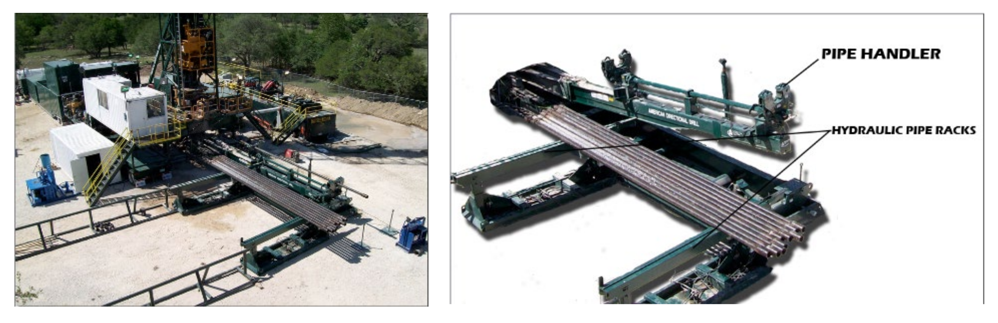
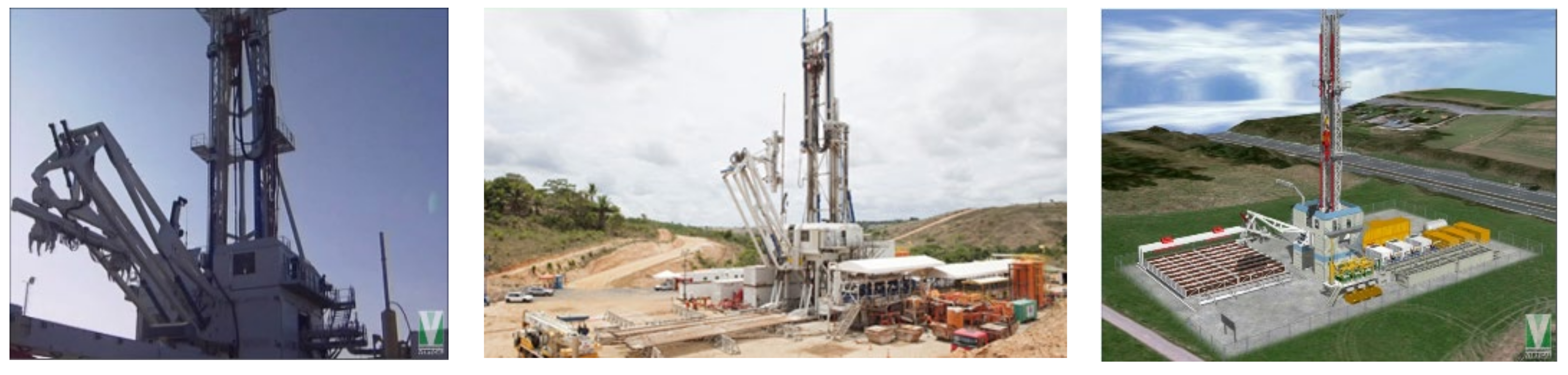
1. Introduction

During the drilling and repairing of wells, the round trip and discharge operations of the drilling rod, casing, and pipe string are usually carried out. Especially in the round-trip process, the discharge operation of a drill string needs to be repeated many times. The characteristics of this kind of equipment are a large work scope and harsh environment. Because the length of the large arm is related to the derrick, the elastic deformation, vibration, and parameters of the arm in the “flexible macro-rigid micro” system [1,2] during the rotation operation will affect the movement accuracy, response speed, controllability, etc., which is the core issue of pipe string moving devices [3,4,5].

Figure 1 shows a string transportation system with the mechanical arm of the gear rack rig of horizontal well drillers (HWDs). The system can grab and lift different sizes of string (drill rod, casing, and drill collar), as well as cooperate with the gear rack rig well, which makes it suitable for small- and medium-sized rigs with low rig heights. The Terra Invader 350 rig of HERRENKNECHT VERTICAL is shown in Figure 2. The base of the discharge system of the rig is fixed to the second deck. It has high automation with a remote control. The second floor may be built high and is most suitable for a deep well rig.

The core issues of the flexible mechanical arm are modeling and solving. The dynamics of multi-body systems were first researched in the 1960s. Only after the 1980s did the study of multi-body system dynamics focus on multi-flexible systems [6]. There are two main modeling methods of flexible mechanism dynamics [7,8] namely vector mechanics methods and analytical mechanics methods. Early studies were mainly focused on the Newton–Euler [9] method. In addition, the Lagrange equation, Hamilton [10,11] principle, and Kane equation have been widely used in the analysis of flexible robot dynamics. Naganathan [12] proposed the kinetic model of the planar flexible mechanism with the Newton–Euler method and Timoshenko beam theory. This method was used to model the flexible mechanism by Kane and Huston, among others. The Lagrange equation and the Hamilton principle use energy to establish the dynamic equation, which can avoid the internal force between adjacent bodies; it is suitable for the simple dynamic analysis of flexible many-body systems. Luca [13] established a closed dynamic equation for a planar flexible robot with the Lagrange equation. Benati proposed the modeling method of general flexible many-body systems based on the Hamilton principle.

In the research areas of flexible robot dynamics and FEM, finite element kinematic and dynamic formulation was successfully developed by Chu A My [14,15] and validated for a flexible robot via the use of a transformation matrix to describe the kinematics of both the joint motion and the link deformation. The authors of [16] developed a new mathematical approach for the dynamic modeling of a general flexible/rigid robot. The proposed approach is applicable to both flexible robots and hybrid flexible/rigid robots. The authors of [17] proposed a systematic algorithm capable of deriving the equations of motion of N-flexible link manipulators with revolute–prismatic joints. The coupling effects due to the simultaneous rotating and reciprocating motions of the flexible arms, as well as the dynamic interactions between large movements and small deflections are also included. Additionally, the effects of gravity and the longitudinal, transversal, and torsional vibrations were considered in the formulations. The authors of [18] presented a systematic modeling procedure based on homogeneous transformation matrices for spatial multilink flexible manipulators with both revolute and prismatic joints. A model-based decoupling control law was used to compare the dynamic responses of the manipulator system.

The coupling of the pipe string transportation device mainly comprises the rigid–flexible coupling dynamics of the mechanical arm and hands [19,20,21]. Based on the “flexible macro-rigid micro” finite element model, we carried out the modeling and numerical simulation of rigid–flexible coupling to investigate the influence of operating parameters and structure parameters on lifting characteristics and to reveal the rigid–flexible coupling mechanism [22]. We described the main factors affecting the vibration characteristics of a flexible arm and modeling conditions of a multi-body system. The results obtained from the simulation will have practical significance in design improvement and the control of the mechanism.

2. Methodology

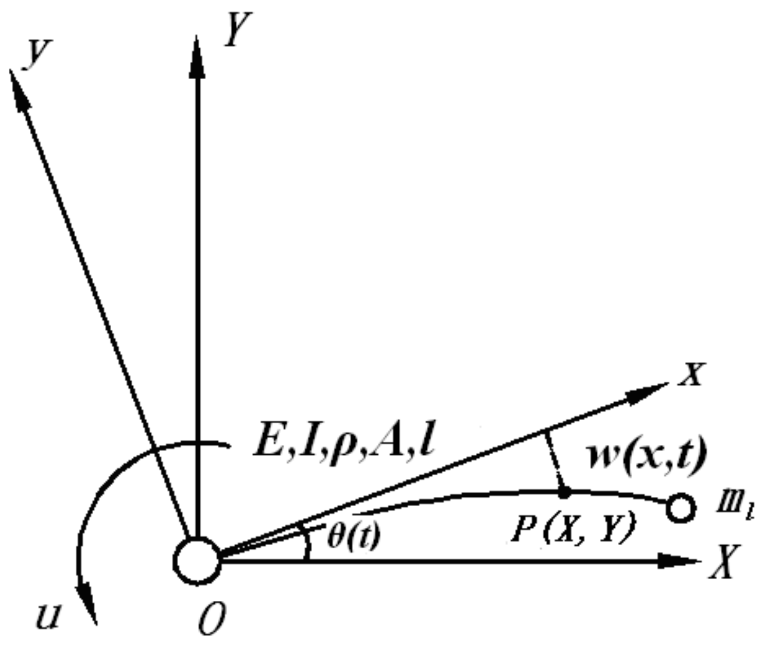
2.1. Kinematics Equation of a Mechanical Arm

The following assumptions were made for the flexible mechanical arm:

(1)

On the premise of small deformation, the influence of shear deformation and the rotational inertia of the section about the neutral axis was ignored;

(2)

The radius of the rotating shaft was ignored;

(3)

The rotating shaft was rigid, and the joint between the beam and the rotating shaft was the hinge support boundary condition;

(4)

The size of the end manipulator was ignored and considered a particle.

A mathematical model of the flexible mechanical arm was built and is shown in Figure 3.

In the figure, XOY is the fixed coordinate system, xOy is the dynamic coordinate system, w(x,t) is the elastic deformation at any point P(X,Y) at time t on the flexible arm, l is the length of the flexible arm, E is the elastic modulus of the material, I is the moment of inertia of the section to the neutral axis, ρ is the arm’s density, θ is the rigid body angle of the flexible arm, m_l is the concentrated mass, and u is the control torque.

For elastic deformation w(x,t), the mode analysis method of dynamic substructure [23] is used to describe the elastic deformation with the modal coordinates. The curved free vibration differential equation [24] is as follows:

$$\rho A\frac{{\partial }^{2}w(x,t)}{\partial t^2}+EI\frac{{\partial }^{4}w(x,t)}{\partial x^4}=0$$

(1)

where

w(x,t) = W(x)q(t)

(2)

where W(x) is the vibration amplitude function at x and q(t) is a time function describing the motion.

Equation (2) can be substituted into Equation (1) to obtain

$$\rho AW(x)\frac{d^{2}q(t)}{d{t}^2}+EI\frac{d^{4}W(x)}{d{x}^4}q(t)=0$$

(3)

or

$$\frac{W^{(4)}(x)}{W(x)}=-\frac{\rho A}{EI}\cdot \frac{\ddot{q}(t)}{q(t)}$$

(4)

Equation (4) holds only if both sides are equal to a constant independent of time and space; this is recorded as λ⁴.

$${\omega }^2=\frac{EI}{\rho A}{\lambda }^4$$

Then, two independent ordinary differential equations can be obtained:

$$\frac{d^{4}W(x)}{d{x}^4}-{\lambda }^{4}W(x)=0$$

(5)

$$\frac{d^{2}q(t)}{d{t}^2}+{\omega }^{2}q(t)=0$$

(6)

By solving Equations (5) and (6), the free vibration solution of the flexible arm can be obtained as follows:

$$W(x)=a_1\sin \lambda x+a_{2}sh\lambda x+a_3\cos \lambda x+a_{4}ch\lambda x$$

(7)

$$q(t)=b_1\cos \omega t+b_2\sin \omega t$$

(8)

The main components of the mechanical arm are simplified, and its mass and position distribution are as shown in Figure 4. The load on the arm includes the mass of the arm itself m_k, the mass of mechanical hands m_n and m_l, and the string mass m_p. Based on boundary conditions, the calculations can be continued as follows.

At hinged end, the deflection is 0 and the bending moment is u; then,

$$w\left(0,t\right)=0$$

(9)

$$EI\frac{{\partial }^{2}w(0,t)}{\partial x^2}=u$$

(10)

where $u=(m_{l}l\frac{{\partial }^{2}w(l,t)}{\partial t^2}+m_{n}n\frac{{\partial }^{2}w(n,t)}{\partial t^2}+m_{k}k\frac{{\partial }^{2}w(k,t)}{\partial t^2}+m_{p}k\frac{{\partial }^{2}w(p,t)}{\partial t^2})\cos \theta$.

At the free end, the bending moment is 0 and has shear balance, so

$$EI\frac{{\partial }^{2}w(l,t)}{\partial x^2}=0$$

(11)

$$EI\frac{{\partial }^{3}w(l,t)}{\partial x^3}=m_l\frac{{\partial }^{2}w(l,t)}{\partial t^2}\cos \theta$$

(12)

Thus, the inherent frequency is

$${\omega }_i={(\frac{{\lambda }_i}{l_1})}^2\sqrt{\frac{EI}{\rho A}}{,}_{{}_{}}{}_{}i=1,2,\cdots$$

(13)

where l₁ is the average value of l, n, k, and p. By solving Equations (9)–(12), the vibration shape function can be expressed as

$$\begin{array}{r}{W}_i\left(x\right)=K[\left(\cos {\lambda }_{i}x-ch{\lambda }_{i}x\right)+\frac{(X_4-X_3)sh{\lambda }_{i}l-X_2(ch{\lambda }_{i}l+\cos {\lambda }_{i}l)}{X_{1}sh{\lambda }_{i}l+X_2\sin {\lambda }_{i}l}\sin {\lambda }_{i}x+\\ \frac{(X_4-X_3)\sin {\lambda }_{i}l+X_1(ch{\lambda }_{i}l+\cos {\lambda }_{i}l)}{X_{1}sh{\lambda }_{i}l+X_2\sin {\lambda }_{i}l}sh{\lambda }_{i}x]\end{array}$$

(14)

where

$$\begin{array}{l}{X}_1=m_{l}l\sin \lambda l+m_{n}n\sin \lambda n+m_{k}k\sin \lambda k+m_{p}p\sin \lambda p\\ X_2=m_{l}lsh\lambda l+m_{n}nsh\lambda n+m_{k}ksh\lambda k+m_{p}psh\lambda p\\ X_3=m_{l}l\cos \lambda l+m_{n}n\cos \lambda n+m_{k}k\cos \lambda k+m_{p}p\cos \lambda p\\ X_4=m_{l}lch\lambda l+m_{n}nch\lambda n+m_{k}kch\lambda k+m_{p}pch\lambda p\end{array}$$

Then, the relative elastic deformation can be described as

$$w(x,t)={\displaystyle \sum _{i=1}^{\infty }{W}_i}(x)q_i(t)$$

(15)

where W_i(x) is the vibration mode function and q_i(t) represents the modal coordinates.

In practice, a higher precision can also be obtained by retaining an appropriate finite modal [25]. Thus, Equation (15) can be written as

$$w(x,t)={\displaystyle \sum _{i=1}^N{W}_i}(x)q_i(t)$$

(16)

where N is the former N order mode used.

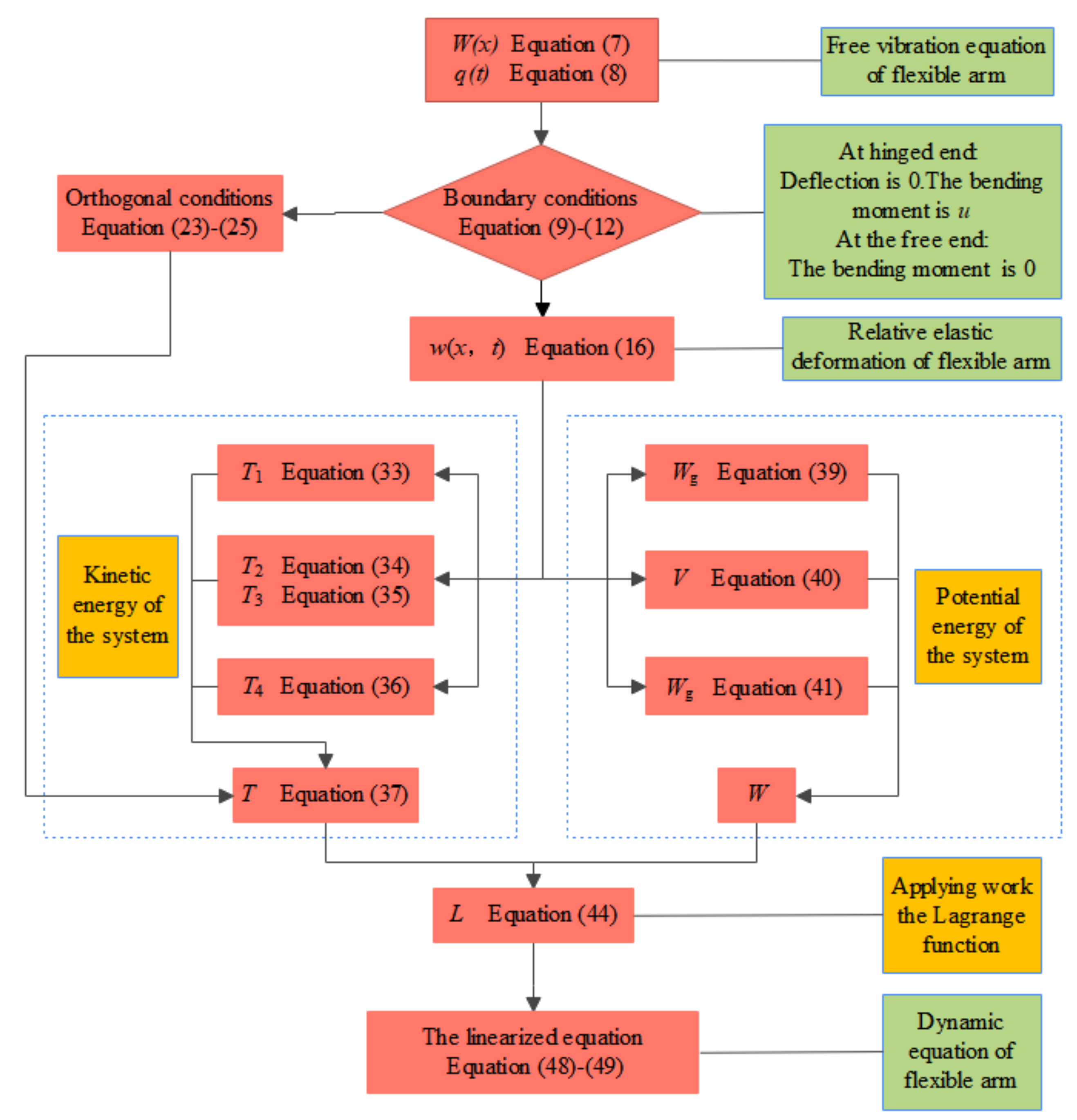
2.2. Dynamic Equation of a Mechanical Arm

We ignored the weight of the hydraulic cylinder and regarded the two mechanical hands and string as a whole, the mass of which (m) can derived as m = m_n + m_k + m_p.

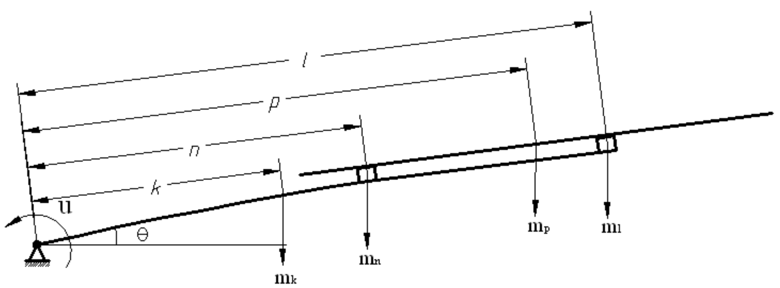
2.2.1. External Load of the Flexible Arm

1.

Single-point force and torque

The single-point force and torque are expressed in the generalized coordinates K:

$$F_K={[0,-mg,0]}^T,T_K={[0,0,0]}^T$$

(17)

Generalized force $Q={\left[Q_T{{}_{}}_{}{Q}_R{{}_{}}_{}{Q}_M\right]}^T$ comprises generalized flat forces, generalized torque, and generalized modal force. Here,

$$Q_T=F_K={[0,-mg,0]}^T$$

(18)

Because of T_K = 0, $Q_R={\left[\begin{array}{ccc}0& 0& 0\end{array}\right]}^T$ and $Q_M={\left[\begin{array}{ccc}0& \dots & 0\\ ⋮& \ddots & ⋮\\ 0& \cdots & 0\end{array}\right]}^T$, so

$$Q={\left[\begin{array}{c}-mg\\ 0\\ ⋮\\ 0\end{array}\right]}^{}$$

(19)

2.

Distributed load

The equation of motion [26] is

$$M\ddot{x}+Kx=F$$

where M and K are the mass and stiffness matrices, respectively, of finite elements on the flexible body, and x and F are the freedom and load vectors, respectively, of the physical nodes [27].

Using Equation (5) of the separation variable method, we can obtain

$$\rho A{\omega }_i{}^2{W}_i(x)=EI\frac{d^{4}W(x)}{d{x}^4}$$

(20)

We then multiply both sides of Equation (20) by W_j(x) and integrate with respect to x along arm length. Via the sub-step integration method [28], we can obtain:

$$\begin{array}{l}\rho A{\omega }_i{}^2{\displaystyle {\int }_0^l{W}_i(x)W_j(x)}dx=EI{\displaystyle {\int }_0^l\frac{d^4{W}_i(x)}{d{x}^4}}{W}_j(x)dx\\ \begin{array}{c}=EI[W_j(x)\frac{d^3{W}_i(x)}{d{x}^3}\left|{}_0^l\right.-\frac{d{W}_j(x)}{dx}\frac{d^2{W}_i(x)}{d{x}^2}\left|{}_0^l\right.]\end{array}+EI{\displaystyle {\int }_0^l\frac{d^2{W}_i(x)}{d{x}^2}}\frac{d^2{W}_j(x)}{d{x}^2}dx\end{array}$$

(21)

Equations (9)–(12) are substituted into Equation (21) to obtain

$$EI{\displaystyle {\int }_0^l\frac{d^2{W}_i(x)}{d{x}^2}}\frac{d^2{W}_j(x)}{d{x}^2}dx=2{\omega }_i{}^2[\rho A{\displaystyle {\int }_0^l{W}_i(x)W_j(x)dx+m_l{W}_i(l)W_j(l)+}{m}_n{W}_i(n)W_j(n)+m_p{W}_i(p)W_j(p)]$$

(22)

Because i and j are arbitrary, when i≠j,ω_i≠ω_j,

$$\rho A{\displaystyle {\int }_0^l{W}_i(x)W_j(x)dx+m_l{W}_i(l)W_j(l)+}{m}_n{W}_i(n)W_j(n)+m_p{W}_i(p)W_j(p)=0$$

(23)

and

$$EI{\displaystyle {\int }_0^l\frac{d^2{W}_i(x)}{d{x}^2}}\frac{d^2{W}_j(x)}{d{x}^2}dx=0$$

(24)

Equations (23) and (24) are the orthogonal conditions of the intrinsic vibration function of the flexible mechanical arms with a concentrated mass at the end.

When $i=j$ in Equation (22), we obtain

$$EI{\displaystyle {\int }_0^l[\frac{d^2{W}_i(x)}{d{x}^2}}{]}^{2}dx=2{\omega }_i{}^2[\rho A{\displaystyle {\int }_0^l{W}_i{}^2(x)dx+m_l{W}_i{}^2(l)+}{m}_n{W}_i{}^2(n)+m_p{W}_i{}^2(p)]$$

(25)

where

$$2[\rho A{\displaystyle {\int }_0^l{W}_i{}^2(x)dx+m_l{W}_i{}^2(l)+}{m}_n{W}_i{}^2(n)+m_p{W}_i{}^2(p)]=M_i$$

(26)

$$EI{\displaystyle {\int }_0^l[\frac{d^2{W}_i(x)}{d{x}^2}}{]}^{2}dx=K_i$$

(27)

Following Equation (25), we can obtain

$$K_i={\omega }_i{}^2{M}_i$$

(28)

where $M_i$ and $K_i$ are the generalized mass and generalized stiffness, respectively, of the ith mode of the flexible mechanical arm.

2.2.2. Energy of the System

1.

Kinetic energy of the system

The total kinetic energy T of the rigid–flexible coupling system includes the kinetic energy of the flexible arm T₁, the kinetic energy of two masses T₂ and T₃, and the kinetic energy of the string T₄:

$$T=T_1+T_2+T_3+T_4$$

(29)

Considering the position, orientation, and mode of the node before and after the deformation, the generalized coordinates of the arm can be represented as [29]

$$\xi ={[\theta ,q_1,\cdots ,q_N]}^T$$

(30)

The velocity formula is expressed in the time derivative $\dot{\xi }$ as

$$v_P=\left[I_{}{}_{}-A\left(s_P+u_P\right)B_{}{}_{}A{\Phi }_P\right]\dot{\xi }$$

(31)

Thus,

$$v_p{}^2=(x^2+w^2(x,t)){\dot{\theta }}^2+{\dot{w}}^2(x,t)-2\dot{\theta }x\dot{w}(x,t)$$

(32)

Equation (32) can be used to calculate T₁, and the kinetic energy of the flexible arm can be obtained as

$$T_1=\frac{1}{2}\rho A{\displaystyle {\int }_0^l[(x^2+w^2(x,t)){\dot{\theta }}^2+{\dot{w}}^2(x,t)-2\dot{\theta }x\dot{w}(x,t)]}dx$$

(33)

The kinetic energy of the two concentrated masses at the end is

$$T_2=\frac{1}{2}{m}_n[(n^2+w^2(n,t)){\dot{\theta }}^2+{\dot{w}}^2(n,t)-2\dot{\theta }n\dot{w}(n,t)]$$

(34)

$$T_3=\frac{1}{2}{m}_l[(l^2+w^2(l,t)){\dot{\theta }}^2+{\dot{w}}^2(l,t)-2\dot{\theta }l\dot{w}(l,t)]$$

(35)

The kinetic energy of the string is

$$T_4=\frac{1}{2}{m}_n[(n^2+w^2(n,t)){\dot{\theta }}^2+{\dot{w}}^2(n,t)-2\dot{\theta }n\dot{w}(n,t)]$$

(36)

Equation (16) can be substituted into Equations (33)–(36); then, the total kinetic energy of the flexible arm can be obtained with orthogonal condition Equations (23)–(25).

$$\begin{array}{l}T=\frac{1}{2}(\rho A{\displaystyle {\int }_0^l{x}^{2}dx+m_l{l}^2+m_n{n}^2+}{m}_p{p}^2){\dot{\theta }}^2+\frac{1}{4}{\displaystyle \sum _{i=1}^N{M}_i[\frac{d{q}_i(t)}{dt}}{]}_{}^2+\frac{1}{4}{\dot{\theta }}^2{\displaystyle \sum _{i=1}^N{M}_i{[q_i(t)]}^2}\\ {{}_{}}_{}{}_{}-\dot{\theta }{\displaystyle \sum _{i=1}^N[\rho A{\displaystyle {\int }_0^{l}x{W}_i(x)}dx+m_{l}l{W}_i(l)+m_{n}n{W}_i(n)+m_{p}p{W}_i(p)]}\frac{d{q}_i(t)}{dt}\end{array}$$

(37)

2.

Potential energy of the system

The total potential energy of the system includes the potential energy of the flexible arm W₁ and the potential energy of the two hands and pipe string W₂. W₁ is also divided into gravity and elastic potential energy:

$$W_1=W_g+V$$

(38)

$$W_g={\displaystyle {\int }_W\rho r_p}\cdot gdW={\displaystyle {\int }_0^l\rho Agx\sin (\theta +\widehat{\theta })}dx$$

(39)

where $\widehat{\theta }=\arctan \left(\frac{w(x,t)}{x}\right)$.

The elastic potential energy of the flexible arm can be calculated with Equation (27):

$$\begin{array}{l}V=\frac{1}{2}{\xi }^{T}K\xi \\ {{}_{}}_{}{}_{}=\frac{1}{2}EI{\displaystyle {\int }_0^l{[{\displaystyle \sum _{i=1}^N\frac{d^2{W}_i(x)}{d{x}^2}}{q}_i(t)]}^2}dx\\ {{}_{}}_{}{}_{}=\frac{1}{2}{\displaystyle \sum _{i=1}^N{K}_i{[q_i(t)]}^2}\end{array}$$

(40)

$$W_2=mg\tilde{L}\sin (\theta +{\widehat{\theta }}_L^{})$$

(41)

where $\tilde{L}$ is the total center of gravity position of the mechanical hands and pipe string. We can obtain the total potential energy of the system with Equations (39)–(41):

$$\begin{array}{l}W=W_g+V+W_2\\ \begin{array}{c}={\displaystyle {\int }_0^l\rho Agx\sin (\theta +\widehat{\theta })}dx+\frac{1}{2}{\displaystyle \sum _{i=1}^N{K}_i{[q_i(t)]}^2}+mg\tilde{L}\sin (\theta +{\widehat{\theta }}_L^{})\end{array}\end{array}$$

(42)

Equations (37) and (42) are used in the Lagrangian function [30,31,32]:

$$L=T-W$$

(43)

Thus,

$$\begin{array}{l}L=\frac{1}{2}J{\dot{\theta }}^2+\frac{1}{4}{\displaystyle \sum _{i=1}^N{M}_i[\frac{d{q}_i(t)}{dt}}{]}_{}^2+\frac{1}{4}{\dot{\theta }}^2{\displaystyle \sum _{i=1}^N{M}_i{[q_i(t)]}^2}-\dot{\theta }{\displaystyle \sum _{i=1}^N[\rho A{\sigma }_i+m_{l}l{W}_i(l)+m_{n}n{W}_i(n)]}\frac{d{q}_i(t)}{dt}\\ {{}_{}}_{}{}_{}-\frac{1}{2}{\displaystyle \sum _{i=1}^N{K}_i{[q_i(t)]}^2}-{\displaystyle {\int }_0^l\rho Agx\sin (\theta +\widehat{\theta })}dx-mg\tilde{L}\sin (\theta +{\widehat{\theta }}_L^{})\end{array}$$

(44)

where

$$J=(\rho A{\displaystyle {\int }_0^l{x}^{2}dx+m_l{l}^2+m_n{n}^2})$$

(45)

$${\sigma }_i={\displaystyle {\int }_0^{l}x{W}_i(x)}dx$$

(46)

The Lagrange equation can then be applied [33]:

$$\left\{\begin{array}{l}\frac{d}{dt}\left(\frac{\partial L}{\partial \dot{\xi }}\right)-\frac{\partial L}{\partial \xi }+{\left[\frac{\partial \psi }{\partial \xi }\right]}^T\lambda =Q\\ \psi =0\end{array}\right.$$

(47)

The dynamics linearized equation can be obtained:

$$\left\{\begin{array}{c}J\ddot{\theta }-{\displaystyle \sum _{i=1}^N[\rho A{\sigma }_i+m_{l}l{W}_i(l)+m_{n}n{W}_i(n)+m_{p}p{W}_i(p)]{\ddot{q}}_i+{\displaystyle {\int }_0^l\cos (\theta +\widehat{\theta })\rho Agxdx}+mg\tilde{L}\cos (\theta +{\widehat{\theta }}_L)=mg}\\ -{\displaystyle \sum _{i=1}^N[\rho A{\sigma }_i+m_{l}l{W}_i(l)+m_{n}n{W}_i(n)+m_{p}p{W}_i(p)]\ddot{\theta }+\frac{1}{2}{M}_i{\ddot{q}}_i+K_i{q}_i=0}\end{array}\right.$$

(48)

This equation is then written as a matrix, as shown in Equation (49):

$$M\ddot{\xi }+K\xi =FQ$$

(49)

where $F={\left[1,0,\cdots 0\right]}^T$ and M is

$$\begin{array}{l}M=\left[\begin{array}{cc}J& -(\rho A{\sigma }_i+m_{l}l{W}_i(l)+m_{n}n{W}_i(n)+m_{p}p{W}_i(p))\\ -(\rho A{\sigma }_i+m_{l}l{W}_i(l)+m_{n}n{W}_i(n)+m_{p}p{W}_i(p))& \frac{1}{2}{M}_1\\ \cdots & \cdots \\ -(\rho A{\sigma }_i+m_{l}l{W}_i(l)+m_{n}n{W}_i(n)+m_{p}p{W}_i(p))& 0\end{array}\right.\\ \\ \begin{array}{ccc}\begin{array}{ccc}& & \end{array}& & \end{array}\begin{array}{cccc}& & & \end{array}\begin{array}{cccc}& & & \end{array}\left.\begin{array}{cc}\cdots & -(\rho A{\sigma }_i+m_{l}l{W}_i(l)+m_{n}n{W}_i(n)+m_{p}p{W}_i(p))\\ \cdots & 0\\ \cdots & \cdots \\ \cdots & \frac{1}{2}{M}_N\end{array}\right]\end{array}$$

(50)

The generalized stiffness array K is

$$K=\left[\begin{array}{cccc}[{\displaystyle {\int }_0^l\rho Agx\cos (\theta +{\widehat{\theta }}_{})dx+mg\tilde{L}\cos (\theta +{\widehat{\theta }}_L)]/\theta }& 0& \cdots & 0\\ 0& K_1& \cdots & 0\\ \cdots & \cdots & \cdots & \cdots \\ 0& 0& \cdots & K_N\end{array}\right]$$

(51)

The calculation flow chart is shown in Figure 5.

3. Modeling and Simulation of a Rigid–Flexible Coupling Mechanical Arm

The mechanical arm was meshed in Ansys and converted to an MNF modal neutral file. The neutral file was then used by ADAMS to analyze the modal and to set constraints and drive types [34]. Finally, the rigid–flexible coupling model was completed. The finite element model of the mechanical arm is shown in Figure 6.

The rigid–flexible coupling model of a pipe string transportation device was established in ADAMS. It is shown in Figure 7.

The lifting of the system will produce a complex rigid–flexible coupling vibration. Therefore, the lifting process comprises the continuous generation and degeneration of vibration.

In order to study the characteristics of the coupling system, the mechanism was simplified to three structures (circular, rectangular, and hollow rectangular section) and three rigid mass blocks, as shown in Figure 8. In this paper, they are called arm 1, arm 2, arm 3, block 1, block 2, and block 3, respectively. The research was mainly focused on the influence of lifting speed, the structure of the arm, different loads, drive type, and shock absorption on lifting characteristics.

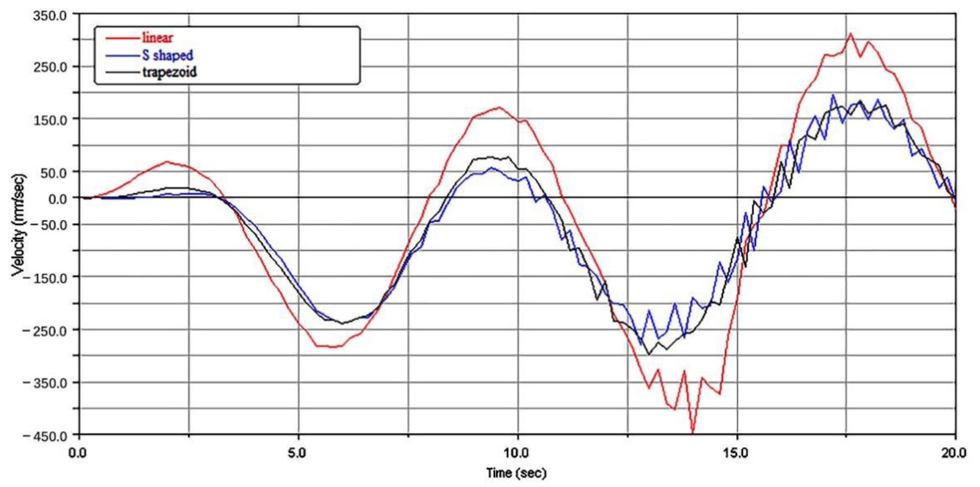
3.1. Simulation Experiment with Different Drive Types

3.1.1. Lifting Characteristics with Different Drive Types

In this simulation, arm 2 and block 2 were selected. According to the productive process, the angular speed drive of uniform speed, trapezoidal curve, and S-curve were adopted with no string and completed the lifting in 15 s to investigate the effect of the drive mode on the lifting characteristics.

The lifting process was completed in the vertical XY 2D plane. After the flexible mechanical arm rises to the vertical position, the vibration of the system is mainly the reciprocating vibration in the X direction. The displacement distribution of the flexible arm is shown in Figure 9. The velocity distribution at the end in the X direction is shown in Figure 10.

In the figure, the displacement of the target position appears as an obvious inflection point with the uniform speed drive. For the other drive, it appears as a smooth transition. It can be seen that the fixed-value drive possesses a large vibration and amplitude, and an S-curve allows for a better control effect than a trapezoidal curve.

A constant value drive will still lead to a large vibration amplitude in the system. All three types of drives were found to manifest as a combination of low-frequency vibration, small fluctuations, and a gradually increasing amplitude. The flexible arm vibration frequency was found to be the same in different driving modes.

It can be concluded that the more gradual a system drives, the stronger its ability to absorb the vibration and the smaller the vibration amplitude will be. For the control of a flexible arm, the mutation led to greater vibration and safety risks and decreased the system’s durability. The vibration frequency of the flexible arm was not found to be affected by each lifting mode. The calculation results of different structures and loads all presented the above-mentioned characteristics.

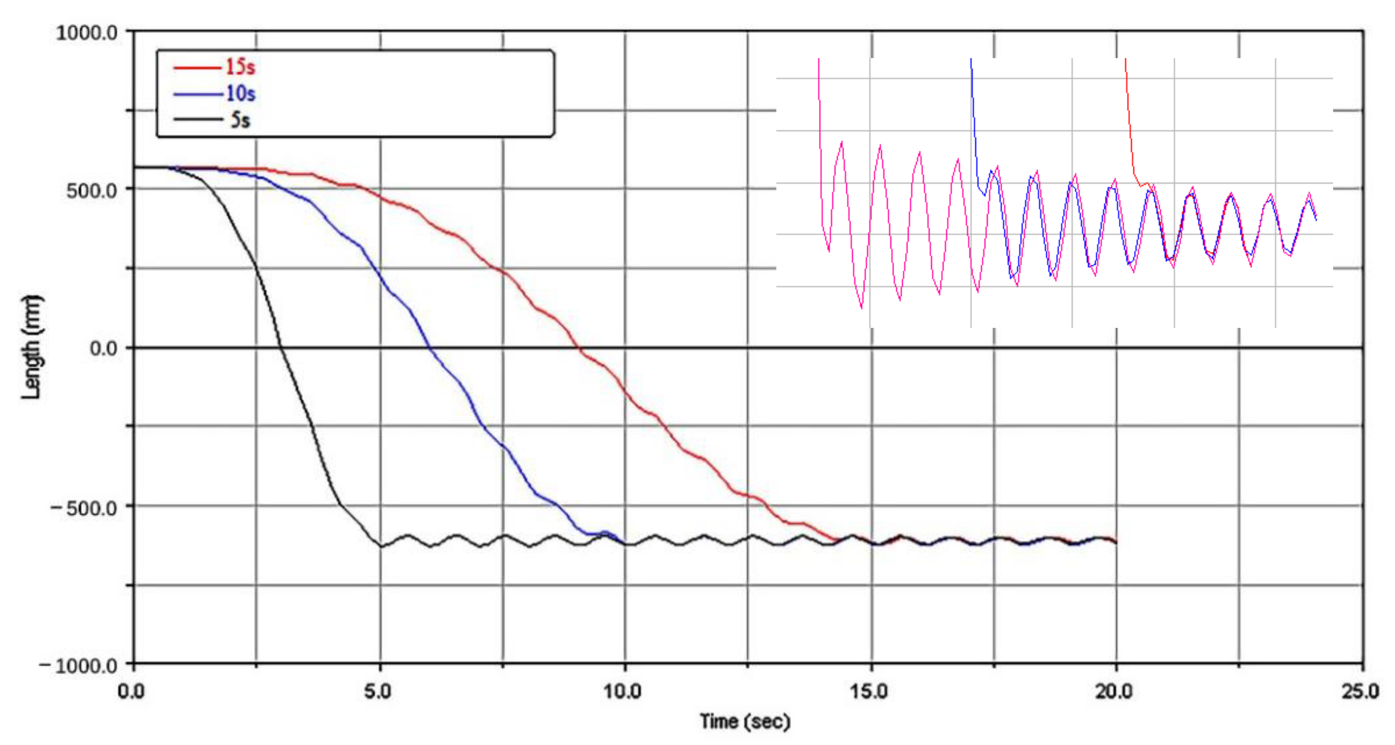
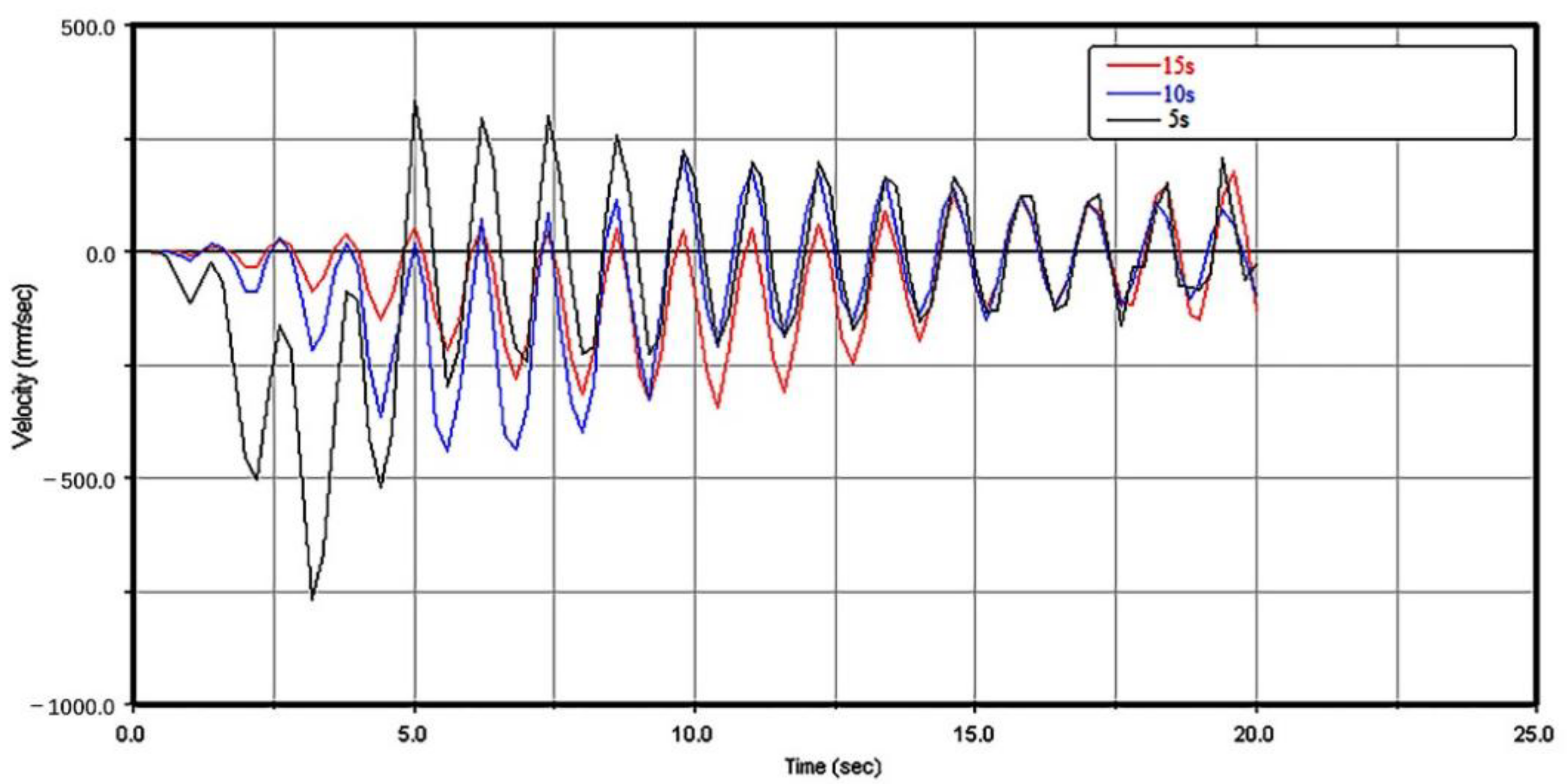
3.1.2. Lifting Characteristics with Different Drive Speeds

In this simulation, arm 1 and block 1 were selected. According to the productive process, lifting times of 15, 10, and 5 s were adopted with no string and the trapezoidal curve drive to investigate the effect of the drive speed on the lifting characteristics. The displacement distribution of different rise speeds is shown in Figure 11. The velocity distribution at the end in the X direction is shown in Figure 12.

It can be seen the larger the lifting speed, the smaller the amplitude, though the vibration frequency did not change. In the target position, a larger lifting speed led to a larger amplitude and a longer vibration decay time. The lifting speed had no effect on the vibration frequency because the inertia force had a significant impact when the lift speed was slightly slow. Therefore, the vibration amplitude of the flexible arm was large. After reaching the vertical position, the system was no longer affected by the lift speed and the vibration frequency was the inherent frequency of the arm.

It can be seen from the velocity diagram that rigid–flexible coupling led to plus–minus velocity alternation. The speed of the flexible arm rose smoothly and the vibration amplitude significantly increased with the rising velocity. The vibration frequency was also not affected by the lift speed. When the lifting time was shortened, the velocity gradient increased, which was not conducive to the stability of the mechanism.

3.2. Simulation Experiment with Different Structure Parameters

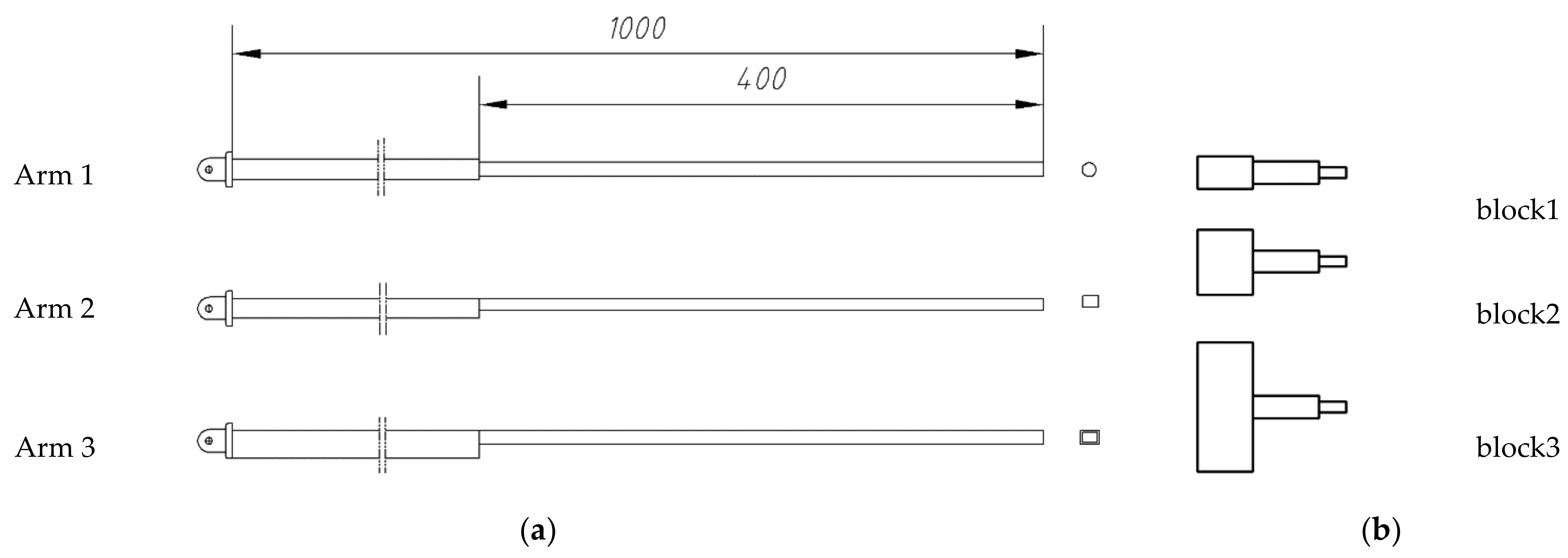
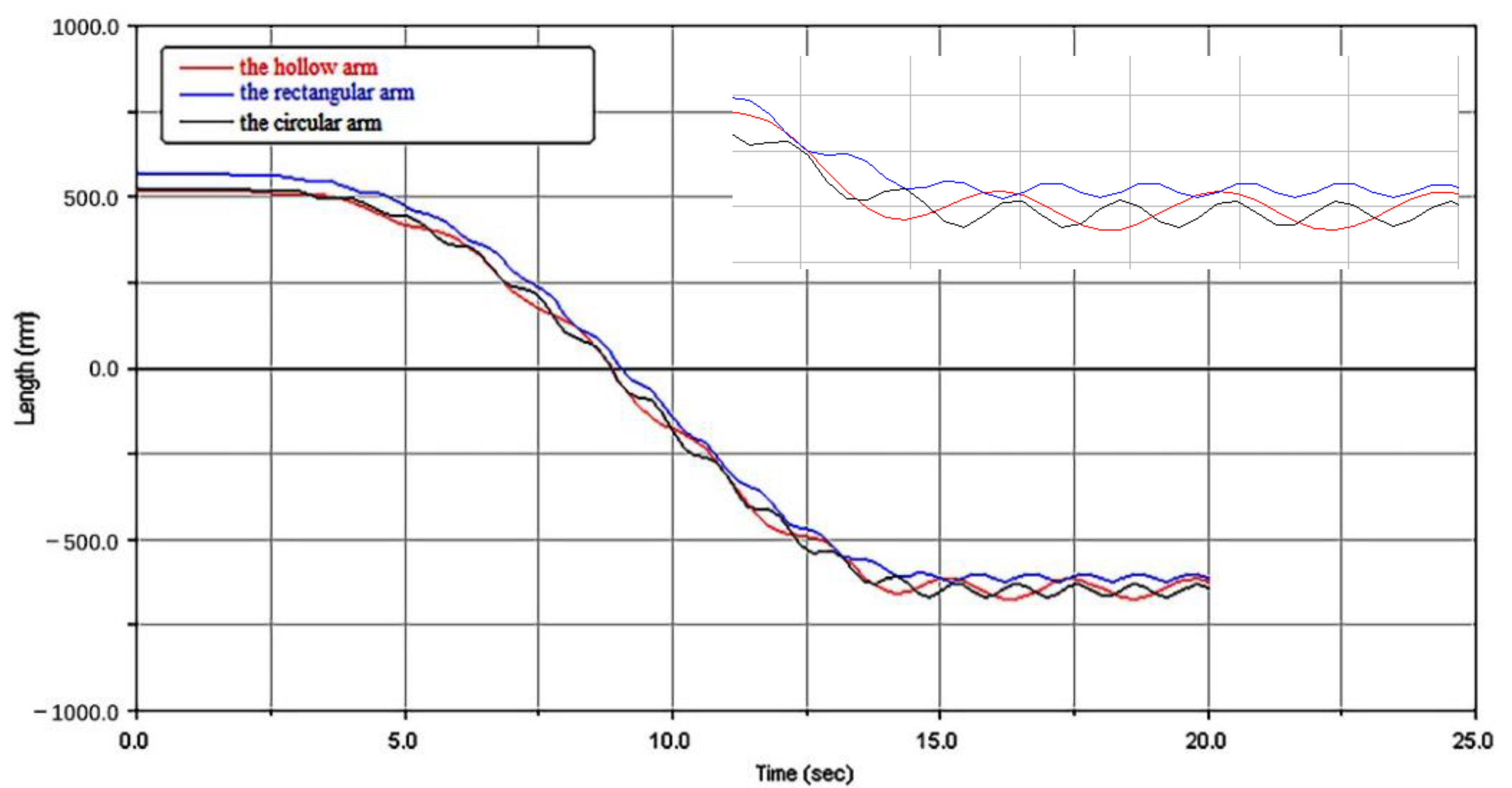
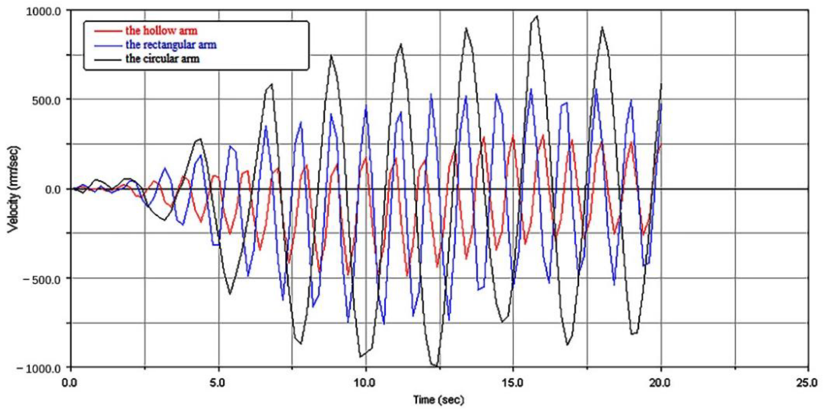
3.2.1. Lifting Characteristics with Different Section Structures

In this simulation, block 3 was selected. In total, three kinds of section structure were adopted with no string, 15 s of lifting time, and the trapezoidal curve drive to investigate their effects on the lifting characteristics. The circular section was found to have the smallest inertia moment (here defined as the inertia moment about the Z axis) and the smallest possible resistance to deformation, the solid rectangular section was found to have the second smallest inertia moment, and the hollow rectangular section was found to have the maximum inertia moment. Additionally, the stiffness of the circular section significantly differed from that of the other two sections. The displacement distribution of the mechanical arm is shown in Figure 13. The velocity distribution at the end in the X direction is shown in Figure 14.

The stiffness was better, the lifting amplitude was smaller, the vibration frequency was faster, and the decay time was shorter for the flexible arm when the inertia moment was large. Because it had strong resistance to deformation when the moment of inertia was large, the deflection at the end of the arm became smaller and the vibration frequency increased. In contrast, the system exhibited opposite vibration characteristics when the moment of inertia was small. At their target position, mechanical arms with a larger inertia moment will take a longer time to absorb vibration.

It can be seen from the velocity diagram that the absolute amplitude of the displacement and velocity increased when the inertia moment of the flexible arm was reduced. This is not conducive to the lifting stability of the mechanism. In addition, a larger inertia moment leads to a larger cross-section and mass, which requires a greater driving force. Therefore, an appropriate arm cross-section should be selected in the actual design.

3.2.2. Lifting Characteristics with Different Loads

In this simulation, arm 3 was selected. Mass blocks of 100, 206, and 412 g were adopted with no string, 15 s of lifting time, and a trapezoidal curve drive to investigate their effects on the lifting characteristics. The displacement distribution of the mechanical arm is shown in Figure 15. The velocity distribution at the end in the X direction is shown in Figure 16.

It can be seen that in the lifting process, the amplitude was larger, and the vibration frequency was smaller when the mass was larger. In the target position, the flexible arm had a larger vibration amplitude, smaller vibration frequency, and a longer decay time when the mass was larger. In contrast, the system exhibited the opposite vibration characteristics when terminal mass was small.

As can be seen from the velocity diagram, the rigid–flexible coupling led to plus–minus velocity alternation. When the end mass was smaller, the system presented a small fluctuation at a low frequency. When the end mass was larger, the absolute amplitude of the displacement and velocity was larger, thus requiring a larger driving force. This case should be avoided as much as possible for flexible arms.

3.3. Simulation Experiment with Hold Strings and Different-Sized Strings

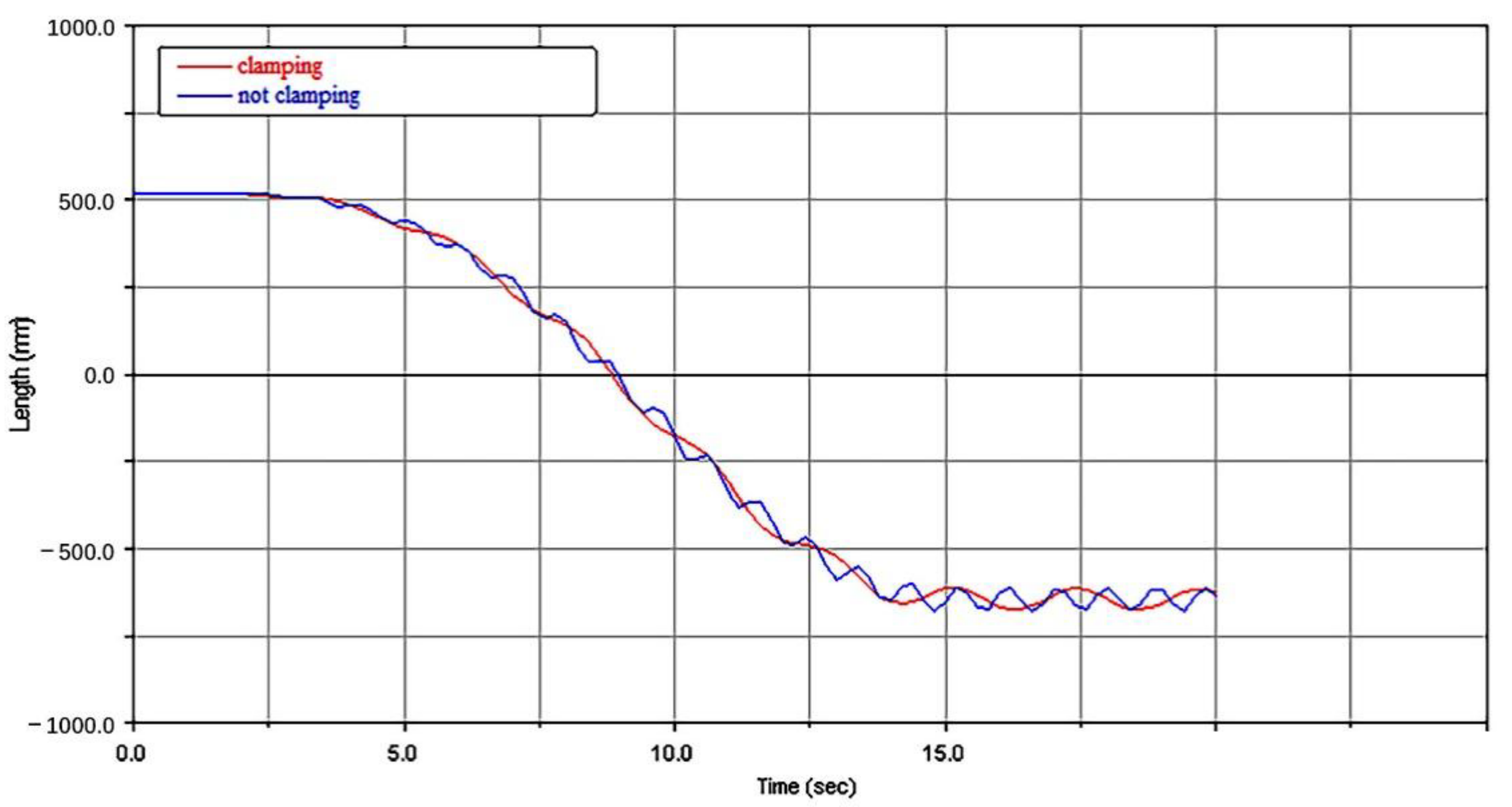
3.3.1. Lifting Characteristics with Clamp String

In this simulation, arm 3 and block 3 were selected. Two states of clamping string and not clamping string were adopted with 15 s of lifting time and the trapezoidal curve drive to investigate their effects on the lifting characteristics. A $2\raisebox{1ex}{$7$}\!\left/ \!\raisebox{-1ex}{$8$}\right.$ inch string was used in the simulation. The model was established with the similarity principle and input into ADAMS.

To determine whether a clamped string would lead to the same arm lifting characteristics with enlargement of the end load, we calculated the displacement distribution of the flexible arm, as shown in Figure 17.

The figure shows that the mechanical arm’s amplitude was larger, the vibration frequency was smaller, and the attenuation time was longer in the lifting process when the string was clamped. At the target position, the vibration amplitude continued. In contrast, the flexible arm without clamping presented a smaller amplitude and faster frequency, which is the same trend observed with an increasing end load. The degree of influence was found to be related to the structure of the arm and the load of the end mass. The clamping of the pipe string was found to have little influence on the end acceleration of the flexible arm.

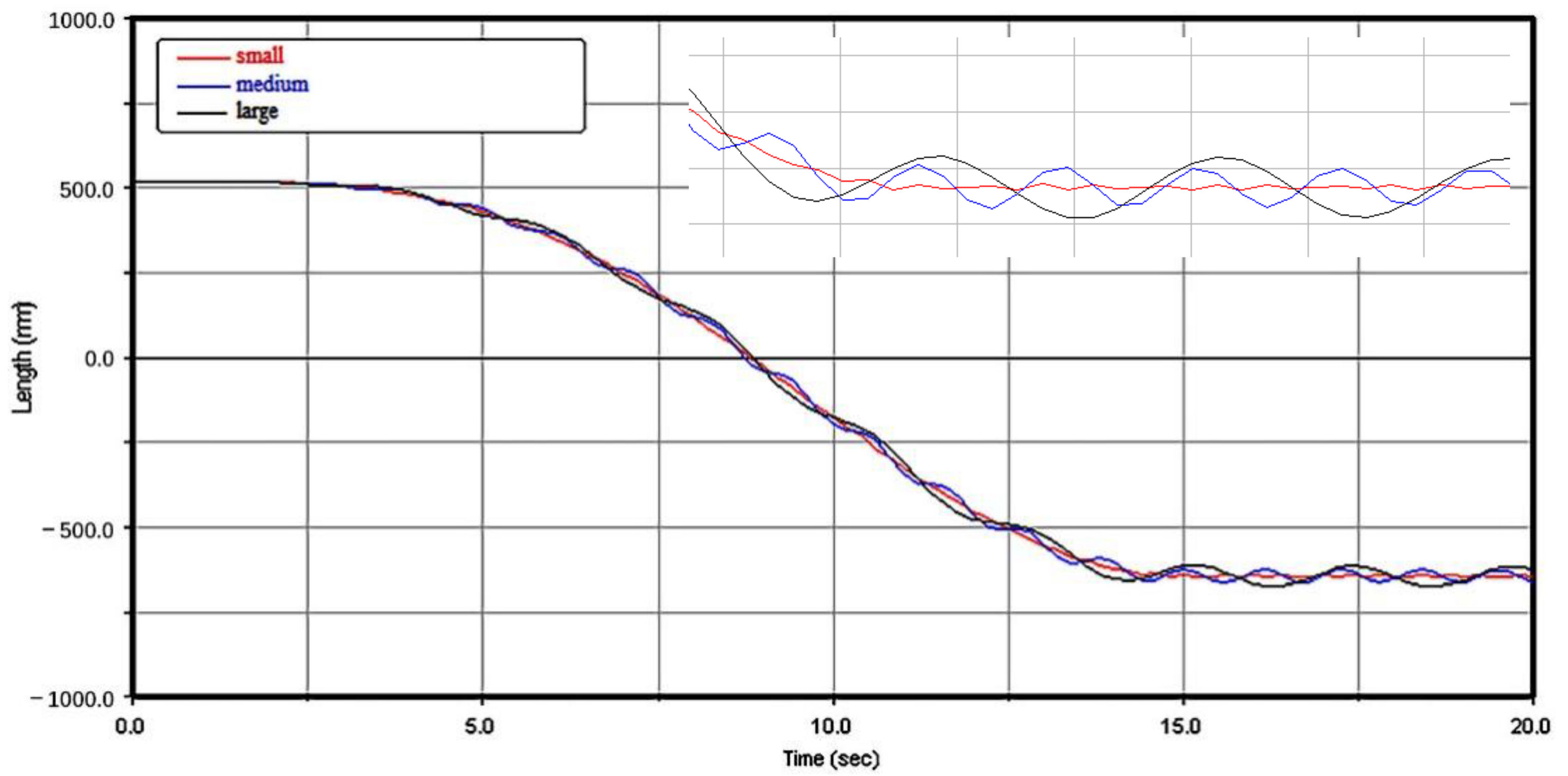
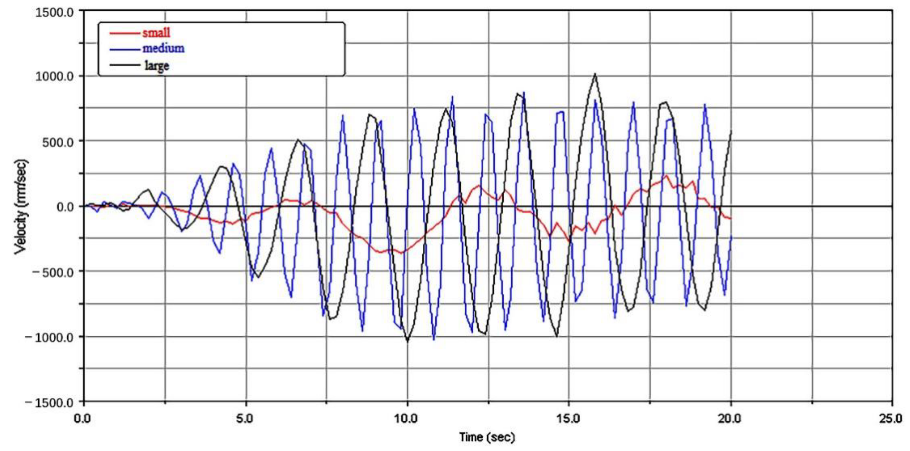
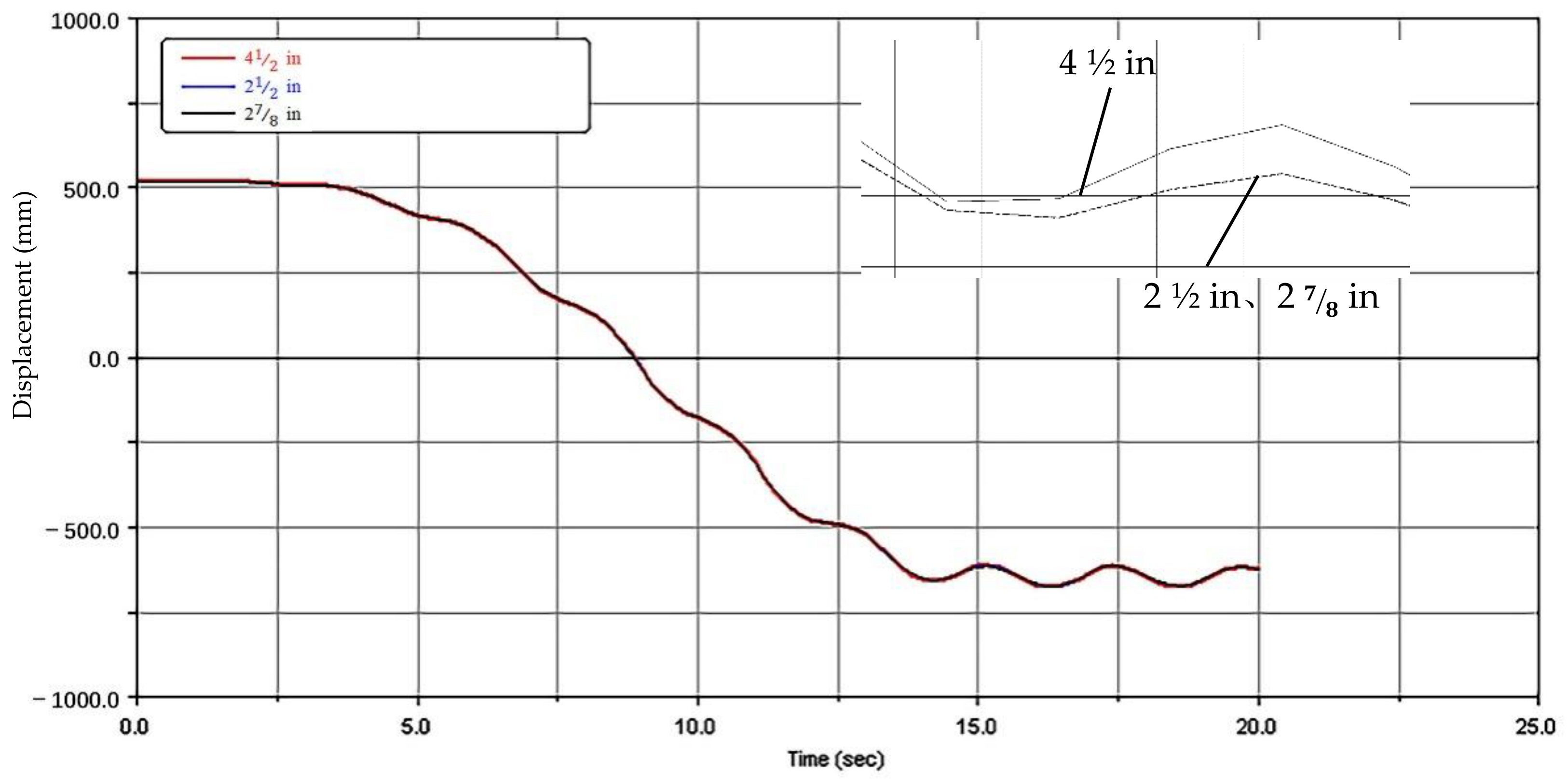
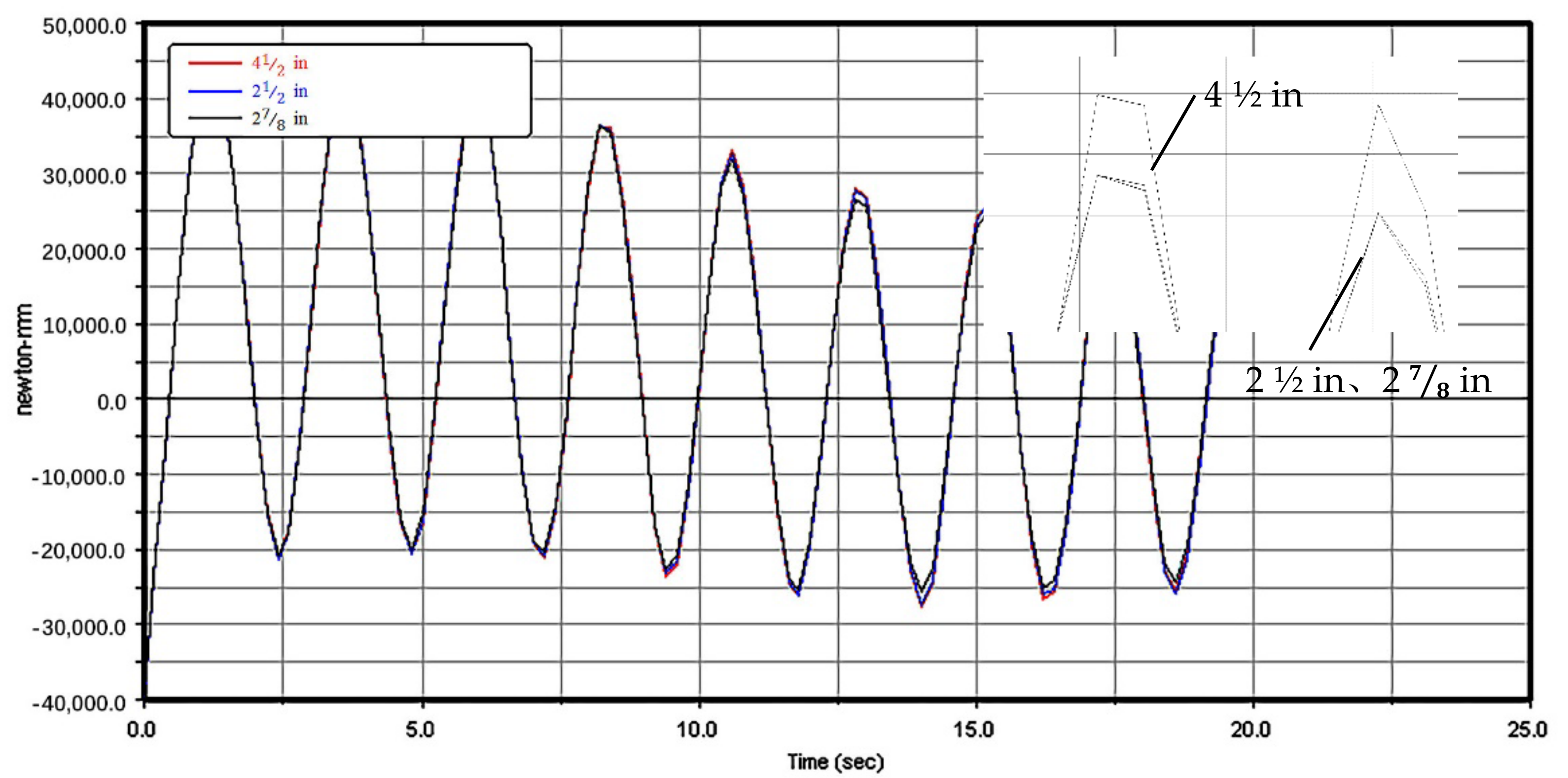
3.3.2. Lifting Characteristics with Different-Sized Strings

In this simulation, arm 3 and block 3 were selected. We adopted strings of $2\raisebox{1ex}{$1$}\!\left/ \!\raisebox{-1ex}{$2$}\right.$, $2\raisebox{1ex}{$7$}\!\left/ \!\raisebox{-1ex}{$8$}\right.$, and $4\raisebox{1ex}{$1$}\!\left/ \!\raisebox{-1ex}{$2$}\right.$ inches with 15 s of lifting time and the trapezoidal curve drive to investigate their effect on the lifting characteristics. The displacement and driving torque distributions for different sizes of string clamped the mechanical arm are shown in Figure 18 and Figure 19, respectively.

It can be seen that the displacement and driving torque curves of the flexible arm with different-sized strings presented only slight differences. The results of the $2\raisebox{1ex}{$1$}\!\left/ \!\raisebox{-1ex}{$2$}\right.$ and $2\raisebox{1ex}{$7$}\!\left/ \!\raisebox{-1ex}{$8$}\right.$ inch strings were the most similar. Specifically, the impact on the flexible arm inevitably increased as the string size increased. However, due to the large dead weight of the system, different pipe string sizes were shown to have little effect on lifting characteristics. Therefore, it is not necessary to change control parameters according to the size of strings.

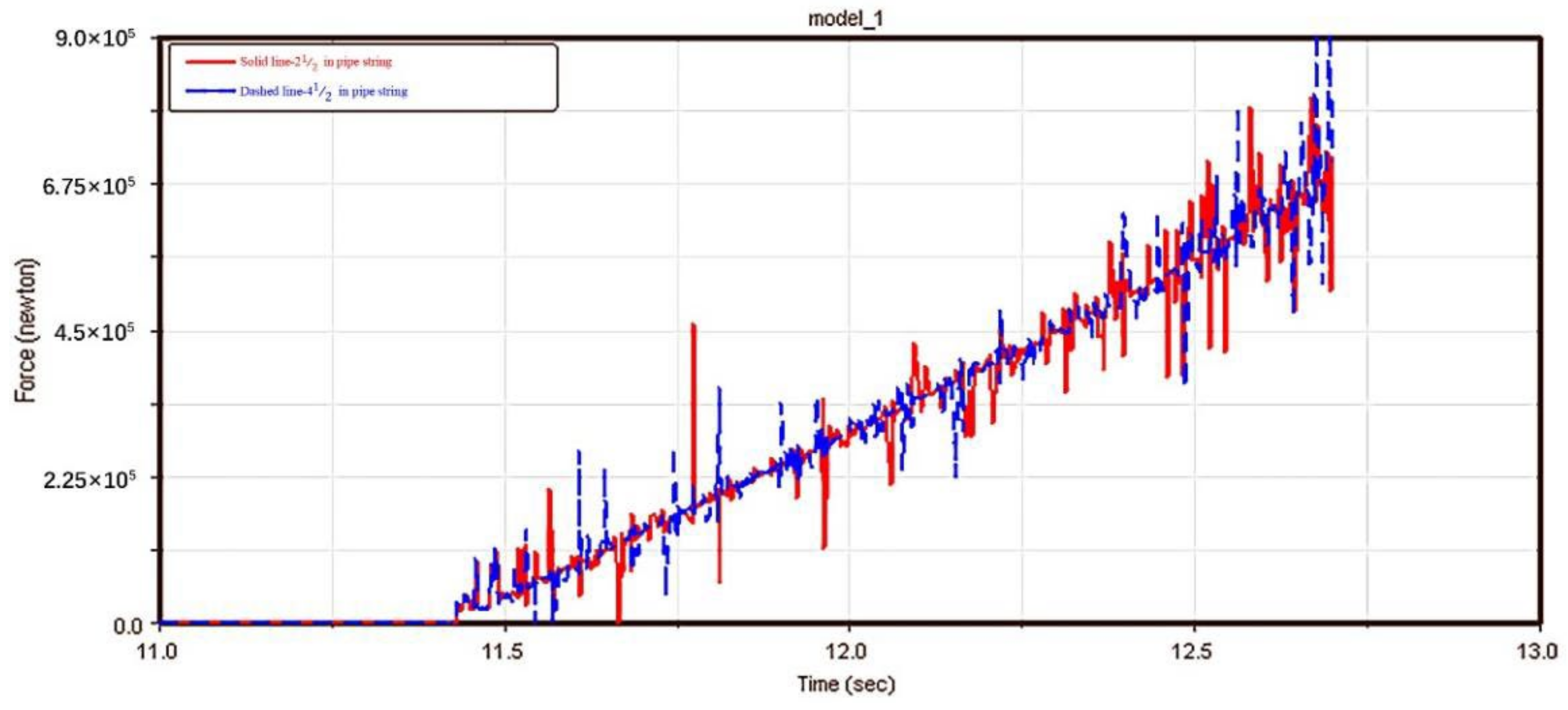
3.4. Contact Collision with Different-Sized Strings

In oil field work, the sizes of pipe string may be different. Accordingly, a $2\raisebox{1ex}{$7$}\!\left/ \!\raisebox{-1ex}{$8$}\right.$ inch string (about 121 kg) and a $4\raisebox{1ex}{$1$}\!\left/ \!\raisebox{-1ex}{$2$}\right.$ inch string (about 200 kg) were adopted for the contact collision simulation analysis of the mechanical arm and dampener [34]. The contact collision force curves are shown in Figure 20.

It can be seen from Figure 20 that the contact collision force did not significantly increase when the weight of the pipe string increased. Except for the slight increase in the collision force at a few points, the change of the collision force was small. The time and magnitude of each collision presented an irregular decay, and the change of string weight had little impact on the vibration characteristics of the system.

4. Discussion

Above all, when a beam moves at high speed in a large range, elastic deformation is inevitable. The error will be large if it is always modeled as a rigid body, especially for the mechanical arm in this article. In reference to experimental data [35], the author found that when elastic deformation was small or the stiffness requirement was not high, it was not necessary to model the system as a flexible body. Bound by [w/l] at 1/650, when [w/l] was in the range of 1/400–1/650, although the mechanism met the stiffness requirements, it was also necessary to model the arm as a flexible body. When [w/l] was between 1/250 and 1/400 because the mechanical arm was a cantilever beam and the allowable stiffness was small, the mechanism easily exceeded the yield limit and produced plastic deformation in the movement process. Accordingly, a mechanical arm must be modeled with a flexible body.

Operation parameters were found to directly affect the stiffness of the arm. Improper parameters can greatly increase the coupling of the movement, increase the elastic deformation, and even produce resonance to reduce the performance of the mechanism. In addition, the operation parameters were found to be related to the arm structure, design requirements, working environment, control systems, and other factors. In short, the only purpose of operation parameter optimization is to ensure that the mechanism runs smoothly and to minimize the impact vibration caused by the elastic deformation on the mechanical arm.

The experimental results show that acceleration is one of the most important operation parameters. Therefore, the following recommendations are provided. If the [w/l] is between 1/650 and 1/1000, the stiffness of the transfer arm is manageable, the driving mode may be trapezoidal, and the acceleration value in the start and stop process should not be greater than 7~8°/s² in order to ensure the controllability of the operation. When the [w/l] is between 1/400 and 1/650, a large elastic deformation may occur, the system can be driven with a trapezoidal curve, and the acceleration should not exceed 5°/s²; furthermore, if S-shaped curve control is adopted, the acceleration value can reach about 9°/s². When [w/l] is between 1/250 and 1/400, the mechanical arm is more flexible and less stiff. Vibration and impact easily occur in the movement process of the mechanism. S-shaped curve control can generally be adopted, and the value of acceleration should not be greater than 7~8°/s².

5. Conclusions

The objectives of this research on the vibration characteristics of a mechanical arm were to study its mechanism of action in order to understand and master its internal laws and to propose relevant technologies and measures to reduce vibration, reduce wear, improve life, and save energy in order to improve the economic and social benefits of the enterprise.

• Based on the theory of flexible dynamics modeling, the orthogonality condition of the natural vibration mode of the mechanical arm with a concentrated mass block at its end was deduced. Then, a numerical calculation model of the rigid–flexible coupling system was established based on the Lagrangian equation.
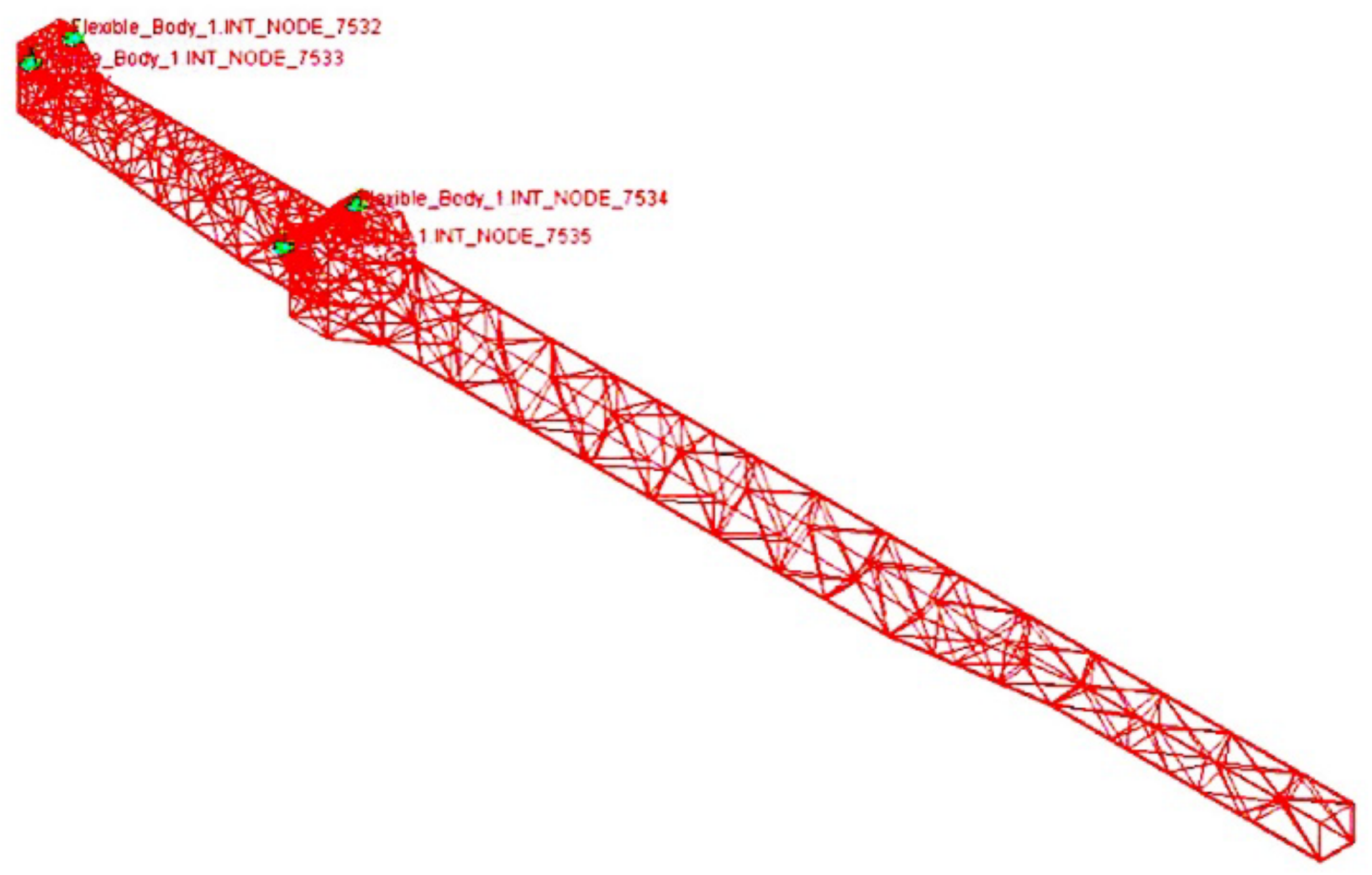
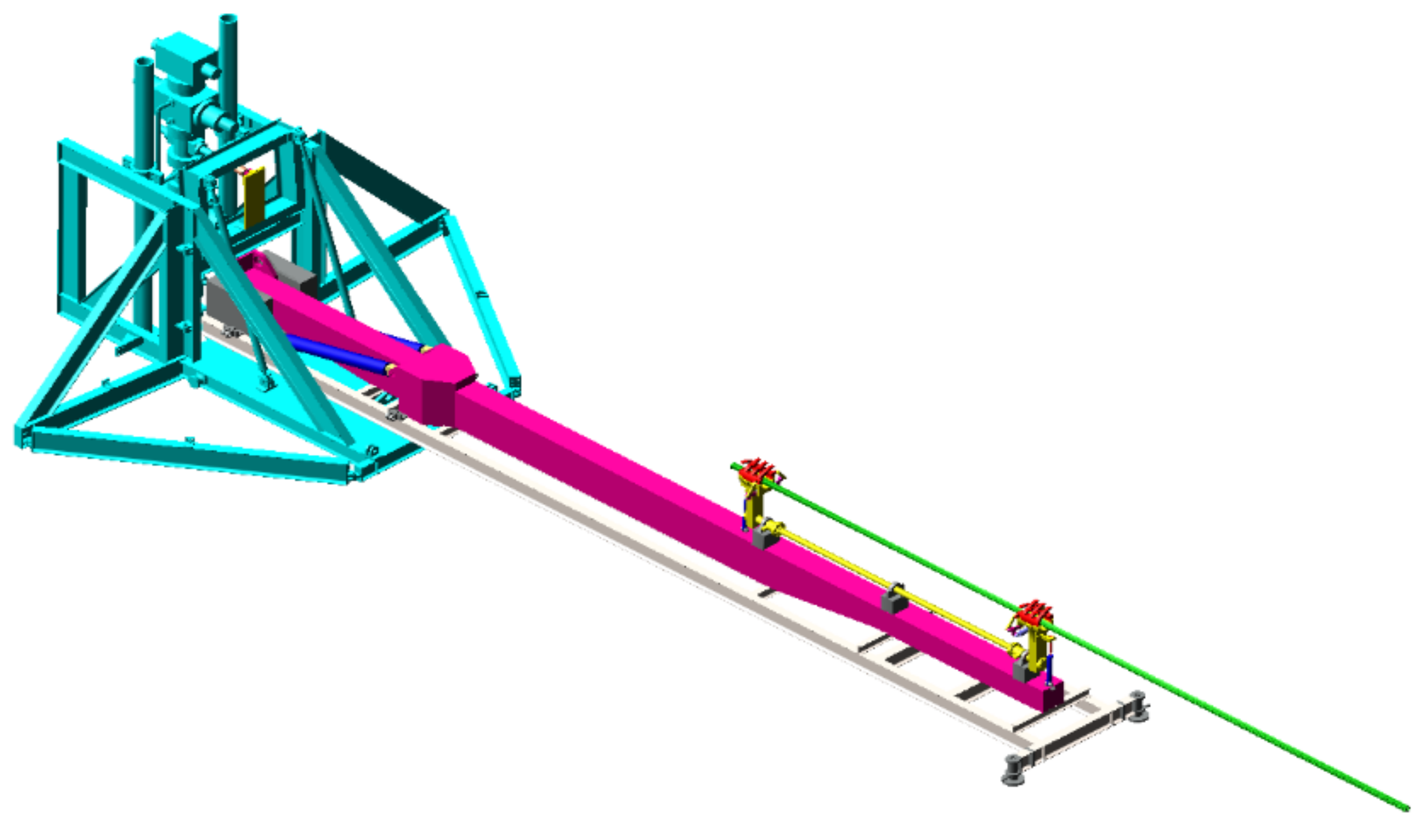
• ADAMS and Ansys were used to carry out the finite element analysis of a rigid–flexible coupling system, and a rigid–flexible hybrid model was established. The lifting process of a mechanical arm was numerically simulated to investigate the lifting characteristics of the flexible arm and the effects of lifting speeds, arm section, and driving modes. The target position and stability of a moving pipe string were calculated. It was concluded that the simulation of flexible parts was close to the reality, and the rigid–flexible coupling analysis was able to reveal the essence of the system.
• The simulation results showed that the weight of the string had little influence on the vibration characteristics. The following considerations should be considered in the design of the mechanism. ① Design parameters such as the weight of the end mass and the structure of the arm have more significant effects on the system than operation parameters. The design of a mechanical arm should first focus on the structure and then optimize the operation parameters of the mechanical arm. ② A flexible arm is characterized by reciprocating vibration lifting, and the vibration amplitude at the end is less than 2% of the total length of the arm. The effect of pipe string transportation and target position were not significant, and compensation from the mechanical hand is unnecessary. ③ The stability problem caused by the vibration of the flexible arm can be greatly reduced with a reasonable shock absorber design and material selection, and an appropriate control method can also quickly attenuate the vibration.
• According to the simulation results, when the design parameter [w/l] of a single-flexible mechanical arm is between 1/650 and 1/1000, the mechanical arm can be modeled as a rigid body. When [w/l] is between 1/400 and 1/650, the rigid–flexible coupling model should be considered for the system. When [w/l] is between 1/250 and 1/400, flexible body modeling should be used for the mechanical arm and the coupling effect of control parameters should be considered.

References

- Lee, H.W. The Study of Mechanical Arm and Intelligent Robot. IEEE Access 2020, 8, 119624–119634. [Google Scholar] [CrossRef]
- Sun, L.N.; Dong, W.; Du, Z.J. Research status and key technologies of macro / micro dual-driven robot system. China Mech. Eng. 2005, 16, 89–93. [Google Scholar]
- Sipos, A.A.; Varkonyi, P.L. The longest soft robotic arm. Int. J. Non-Linear Mech. 2020, 119, 103354. [Google Scholar] [CrossRef]
- Tarnita, D.; Marghitu, D.B. Analysis of a hand arm system. Robot. Comput.-Integr. Manuf. 2013, 29, 493–501. [Google Scholar] [CrossRef]
- Zhu, Y.; Qiu, J.H.; Tani, J. Simultaneous optimization of a flexible robot arm. JSME Int. J. Ser. C-Mech. Syst. Mach. Elem. Manuf. 2000, 43, 32–37. [Google Scholar] [CrossRef] [Green Version]
- Chen, L.P.; Zhang, Y.Q.; Ren, W.Q.; Qin, G. The Mechanical System Dynamics Analysis and the ADAMS Application Tutorial; Tsinghua University Press: Beijing, China, 2005. [Google Scholar]
- Hong, J.Z.; Jiang, L.Z. Flexible multibody dynamics with coupled rigid and deformation motions. Adv. Mech. 2000, 30, 15–20. [Google Scholar]
- Hong, J.Z.; Jiang, L.Z. Dynamic stiffening and multibody dynamics with coupled rigid and deformation motions. Chin. J. Comput. Mech. 1999, 16, 295–301. [Google Scholar]
- Kane, T.R.; Ryan, R.R.; Banerjee, A.K. Dynamics of a cantilever beam attached to a moving base. J. Guid. Control. Dyn. 1987, 10, 139–151. [Google Scholar] [CrossRef]
- Liu, J.Y.; Hong, J.Z. Dynamic modeling and modal truncation approach for a high-speed rotating elastic beam. Arch. Appl. Mech. 2002, 72, 554–563. [Google Scholar] [CrossRef]
- Yan, G.H.; Hong, J.Z.; Yu, Z.Y. Dynamics modeling of a flexible hub-beam system with a tip mass. J. Sound Vib. 2003, 266, 759–774. [Google Scholar]
- Naganathan, G.; Soni, A.H. An analytical and experimental investigation of flexible manipulator performance. In Proceedings of the IEEE International Conference on Robotics and Automation, Raleigh, NC, USA, 31 March–3 April 1987; pp. 767–773. [Google Scholar]
- Luca, A.; Sicilano, B. Closed-form dynamic model of planar multilink light weight robots. IEEE Trans. Syst. Man Cybern. 1991, 21, 826–839. [Google Scholar] [CrossRef]
- My, C.A.; Bien, D.X.; Le, C.H.; Packianather, M. An efficient finite element formulation of dynamics for a flexible robot with different type of joints. Mech. Mach. Theory 2018, 134, 267–288. [Google Scholar] [CrossRef]
- My, C.A.; Bien, D.X. New development of the dynamic modeling and the inverse dynamic analysis for flexible robot. Int. J. Adv. Robot. Syst. 2020, 17, 1–12. [Google Scholar] [CrossRef]
- Chu, A.M.; Nguyen, C.D.; Duong, X.B.; Nguyen, A.V.; Nguyen, T.A.; Le, C.H.; Packianather, M. A novel mathematical approach for finite element formulation of flexible robot dynamics. Mech. Based Des. Struct. Mach. 2020, 1–21. [Google Scholar] [CrossRef]
- Korayem, M.H.; Shafei, A.M.; Dehkordi, S.F. Systematic modeling of a chain of N-flexible link manipulators connected by revolute–prismatic joints using recursive Gibbs-Appell formulation. Arch. Appl. Mech. 2014, 84, 187–206. [Google Scholar] [CrossRef]
- Theodore, R.J.; Ghosal, A. Comparison of the Assumed Modes and Finite Element Models for Flexible Multilink Manipulators. Int. J. Robot. Res. 1995, 14, 91–111. [Google Scholar] [CrossRef] [Green Version]
- Huston, R.L. Multi-body dynamics: Modeling and analysis methods. Appl. Mech. Rev. 1991, 44, 109–117. [Google Scholar] [CrossRef]
- Shabana, A.A. Flexible multi-body dynamics: Review of past and recent developments. Multi-Body Syst. Dyn. 1997, 1, 189–222. [Google Scholar] [CrossRef]
- Schiehlen, W. Multi-body system dynamics: Roots and perspectives. Multi-Body Syst. Dyn. 1997, 1, 149–188. [Google Scholar] [CrossRef]
- Zhang, Y.; Hao, H.Y.; Sun, Z.Q. Esearchon continuous trajectory tracing control of flexible macro-micro space manipulator system. J. Mech. Eng. 2005, 41, 125–131. [Google Scholar] [CrossRef]
- Li, J.T.; Deng, H. Vibration suppression of rotating long flexible mechanical arms based on harmonic input signals. J. Sound Vib. 2018, 436, 253–261. [Google Scholar] [CrossRef]
- He, B.Y.; Wang, S.X. Study on the dynamic model and simulation of a flexible mechanical arm considering its random parameters. J. Mech. Sci. Technol. 2005, 19, 265–271. [Google Scholar] [CrossRef]
- Cai, G.P.; Hong, J.Z. Assumed mode method of a rotating flexible beam. Acta Mech. Sin. 2005, 37, 48–56. [Google Scholar]
- Wang, F.Y.; Gao, Y.Q. Modeling Design Control and Applications: Advanced Studies of Flexible Robotic Manipulators; World Scientific Publishing Co. Pte. Ltd.: London, UK, 2003. [Google Scholar]
- Kang, X.W.; Zhang, Y.; Jiang, L.H.; Han, L.; Chu, H.Q.; Zhu, Q. Study of vibration characteristic of phononic crystals flexible mechanical arms. Optoelectron. Adv. Mater.-Rapid Commun. 2014, 8, 964–967. [Google Scholar]
- Ahmed, A.; Shabana, A. Dynamics of Multibody Systems; The United States of America by Cambridge University Press: New York, NY, USA, 2005. [Google Scholar]
- Liu, Z.Y. Study on Modeling Theory and Simulation Technique for Rigid-Flexible Coupling Systems Dynamics; Shanghai Jiao Tong University: Shanghai, China, 2008. [Google Scholar]
- Song, Y.M.; Yu, Y.Q.; Zhang, C.; Ma, J.S. Summary on the study of dynamics analysis and vibration control of flexible robots. J. Mach. Des. 2003, 20, 1–5. [Google Scholar]
- Liu, S.Z.; Yu, Y.Q.; Du, Z.C.; Liu, Q.B. A summary of the dynamics analysis and control strategy of flexible manipulators. Ind. Instrum. Autom. 2008, 2, 18–24. [Google Scholar]
- Zhang, Y.; Kang, X.W.; Jiang, L.H.; Han, L.; Chu, H.Q.; Zhu, Q. Vibration attenuation in two-link flexible mechanical arms with periodic composite materials. Adv. Mech. Eng. 2015, 7, 1–8. [Google Scholar] [CrossRef] [Green Version]
- Li, J.; Wang, Y.; Zhang, K.; Wang, Z.Q.; Lu, J.X. Design and analysis of demolition robot arm based on finite element method. Adv. Mech. Eng. 2019, 11, 1–9. [Google Scholar] [CrossRef] [Green Version]
- Cheng, D.X.; Wang, D.F.; Liu, S.C.; Ji, K.S.; Han, X.S.; Yu, M.S.; Gao, S.Z.; Ke, R.Z.; Yang, Q.; Liu, Z.J.; et al. Mechanical Design Manual; Chemical Industry Press House: Beijing, China, 2004. [Google Scholar]
- Deng, Z.C.; Wang, X.R.; Zhao, Y.L. Precise control for vibration of rigid-flexible mechanical arm. Mech. Res. Commun. 2003, 30, 135–141. [Google Scholar]
Publisher’s Note: MDPI stays neutral with regard to jurisdictional claims in published maps and institutional affiliations. |
© 2022 by the authors. Licensee MDPI, Basel, Switzerland. This article is an open access article distributed under the terms and conditions of the Creative Commons Attribution (CC BY) license (https://creativecommons.org/licenses/by/4.0/).
Share and Cite
Wang, Y.; Lu, S.; Gao, S.; Ren, Y.; Zhang, R. A Study of the Vibration Characteristics of Flexible Mechanical Arms for Pipe String Transportation in Oilfields. Energies 2022, 15, 2030. https://doi.org/10.3390/en15062030
Wang Y, Lu S, Gao S, Ren Y, Zhang R. A Study of the Vibration Characteristics of Flexible Mechanical Arms for Pipe String Transportation in Oilfields. Energies. 2022; 15(6):2030. https://doi.org/10.3390/en15062030
Chicago/Turabian StyleWang, Yan, Shuwen Lu, Sheng Gao, Yongliang Ren, and Ruijie Zhang. 2022. "A Study of the Vibration Characteristics of Flexible Mechanical Arms for Pipe String Transportation in Oilfields" Energies 15, no. 6: 2030. https://doi.org/10.3390/en15062030