Abstract
This work presents a methodology for horizontal soil stratification and a device for 3D soil mapping using the discretization of the Wenner’s method. The methodology starts from the application of the lateral profiling method in conjunction with the Wenner’s method to find the experimental resistivity curve. The Sunde’s algorithm is used to construct the theoretical resistivity curve. By utilizing these experimental and theoretical resistivity curves, it is possible to apply the optimization process to find the parameters: electrical conductivity and thickness of each soil layer. The area under study is discretized and the results related to all subareas are unified using interpolation process. The whole process which results in 3D soil mapping may be automatically produced using the proposed device.
1. Introduction
Several methods are used for soil mapping according to their approach, invasive or noninvasive, and their purpose, as material identification, physicochemical soil characterization, and others. Regarding the approach, noninvasive methods collect data without changing the structure or dynamics of the soil, which is especially needed in electrical grounding and precision agriculture [1]. Invasive methods make the soil inquiry through excavations, making detailed soil analysis impractical due to the need to collect a large number of samples [2,3].
Soil inquiry through excavations is also not recommended because it causes the fractionation of the entire volume of the soil structure, including its aggregates. Noninvasive methods allow the collection of data from the entire volume in the field without the need to obtain soil samples for laboratory analysis, keeping the soil structure unchanged [1,4]. The soil mapping may be highly accurate depending on the strategy used to collect data in the field [5,6].
In agriculture, the way in which a particular crop plantation is conducted depends on the current geological configuration, once the physical-chemical properties of the soil vary over time due to its relationship with the climatic conditions [7]. The need to consider the soil spatial variability was extensively discussed by the scientists in the geoscience area called precision agriculture, i.e., the way to manage a productive space with spatial detailing to spread different amounts of inputs, since the soil has different properties even in small areas of the field [3].
Precision agriculture has pioneered the use of the concept of Variable-Rate Technology (VRT). This kind of technology is developed by the joint effort of different types of engineering expertise: (i) electrical and electronic; (ii) control and automation; (iii) mechanical; (iv) energy conservation and environmental; and (v) agricultural. VRT refers to any technology that allows the producers to vary the amount of deposited material, its concentration, or its proportion in relation to other materials [3].
One of the basic principles of geophysics used in precision agriculture is based on the soil property of having its electrical conductivity changed due to the variation of its physical-chemical properties. By mapping the electrical conductivity of a soil, areas with homogeneous physical-chemical characteristics may be identified. Therefore, the electrical conductivity values concern to the measurement points that are mapped geographically, making it possible to divide the soil in different management areas [8]. After determining these areas, a soil sample per area is collected for analysis of its physical-chemical properties.
The identification of these management areas combined with their physical-chemical properties allows us to determine the required amount of agricultural inputs, pesticides, and water in irrigation [5]. The electrical conductivity mapping became an effective tool to investigate the behavior and spatial variability of the soil, allowing us to identify areas with similar properties and define differentiated management zones easily [9,10] to apply VRT.
Several methods and types of equipment are used to measure the soil electrical conductivity. Among all the equipment types, the most known of them uses the following principles: (i) electrical resistivity and (ii) electromagnetic induction [11,12]. The stratification methods that apply the electrical resistivity principles are usually modeled by mathematical expressions that consider the soil to be homogeneous; that is, they do not consider the existence of layers and model the apparent electrical conductivity only for constant depth limited by the equipment, which usually depends on the distance between the conductors that inject the electrical current in the ground. In general, the depth values adopted are around m and m, depending on the equipment used [13]. The stratification methods that apply the electromagnetic induction principle also model the soil as homogeneous mass and they map the soil up to m [11].
This superficial analysis is no longer considered sufficient for certain crops and regions, as the root systems of some plants may reach much deeper than m [14,15,16], furthermore, the apparent electrical conductivity readings vary significantly among the several types of devices used for these tasks [17]. Several studies in dry regions showed that there is a rich and active ecosystem in depths [18,19,20] with macro and microorganisms; hence, it is relevant to know the soil up to the depth of the plant root system, which absorbs nutrients from different layers of the subsoil [21,22,23]. Other authors linked the soil electrical conductivity and the thickness of the soil layers, identifying properties such as hydrodynamics and soil compaction [24,25,26].
Another technique used for small area studies (≤0.40 m) is Computed Tomography (CT Scan) [27], a noninvasive imaging technique that enables quantitative analysis of physical properties of materials. This type of study is costly, and it was introduced in soil science for studies of soil density, moisture and water movement measurements, compaction, and soil structure regeneration, among others [28,29,30,31].
Inspired by CT Scan method from the point of view of producing 3D distributions of material characteristics, the motivation of our research is to propose 3D soil mapping to fill a gap in the area of precision agriculture. Unlike 2D prospecting, 3D mapping of soil electrical conductivity (or its inverse, electrical resistivity) yields a complete description of the soil structure, mapping homogeneous layers of variable thicknesses in large areas, thus considering the heterogeneous soil [5].
The techniques used in precision agriculture to determine the value of electrical conductivity consider the soil to be vertically homogeneous and measure the apparent electrical conductivity, considering it constant up to depths in the interval of [0.2; 0.9] meters [17]. The surface analysis of the soil is no longer considered sufficient since the root system of some plants reaches depths greater than the values normally used, thus proposing a mobile device that makes it possible to determine the electrical conductivity and thickness of the soil layers at different depths and accurately, becomes the originality and relevance of this research.
The mobile device proposed in this paper together with the 3D stratification methodology makes use of a farm vehicle and can be used for use in precision agriculture, in soil stratification for construction of electrical grounding meshes, and study of foundations for buildings, thus making the innovation of this work. The device can carry out the soil mapping by determining the electrical conductivity without the need for excavation in the ground, allowing the process of soil stratification in large areas to be carried out dynamically without the financial burden and faster compared to traditional methods, indicating the reasonableness and applicability of the research.
We present a methodology and a device that, combined, are able to perform a 3D mapping of the soil through its resistivity or conductivity without expensive field excavations. Section 2 describes the geoelectrical surveying method used in this work. In Section 3, the proposed mapping methodology is presented and the device developed to collect field data related to stratification and mapping 3D of the soil is described. Section 4 presents the results obtained, and Section 5 concludes with a brief discussion of the results.
2. Theoretical Background
Regardless of the type of arrangement of electrodes used in geoelectric prospecting measurements, there are basically two ways of performing the electrical resistivity measurements: (i) vertical or (ii) horizontal. The choice of which method to use is related to the purpose of the study, however there is a need for both vertical and horizontal investigations to carry out the 3D mapping. To find to the distribution of the apparent electrical resistivity on the soil surface, the lateral profiling method is applied. By using Wenner’s method, the values of a (distance between two consecutive electrodes) are varied to identify soil variations in depth.
This work considers: (i) soil stratification as the process of finding the number of soil layers with their respective values of resistivity and thickness and (ii) 3D soil mapping as the presentation in the graphical form of data obtained and treated after stratification.
2.1. Determination of Apparent Electrical Resistivity of the Soil
The lateral profiling method is the geoelectrical investigation technique used to find the mapping of the apparent electrical resistivity on the soil surface, which consists of placing the arrangement of the electrodes at the measuring spots, keeping fixed the distance between the rods. In this situation, is determined at the center point of the arrangement, between the potential electrodes. Thus, it is possible to map the whole area, identifying the measuring spots and consequently delimiting distinct regions of resistivity [6,7].
Figure 1, adapted from Silva Filho et al. [32], illustrates the lateral profiling method of soil investigation, in which the measurement process of apparent electrical resistivity is performed for the measuring spots given by the intersection between the Column 1 and the Row A, Row B, Row C and Row D. The Wenner’s method is applied in Figure 1, where the current and voltage electrodes are represented by dots in the blue color while the dots in the red color are the measuring spots of . By performing the lateral profiling method along Column 1, Column 2, Column 3 and Column 4, the mapping of the apparent electrical resistivity over the surface of the soil being studied is obtained [33,34].
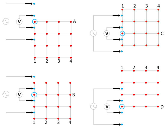
Figure 1.
Application of lateral profiling method.
Soil mapping is used in many areas from civil engineering to precision agriculture. Each area needs to know specific parameters of the subsoil and its dynamics. However, there are parameters that are common to all areas, such as apparent resistivity of the soil (and its inverse to apparent conductivity) and the depths of each layer, illustrated in Figure 2, adapted from Calixto et al. [5,6].
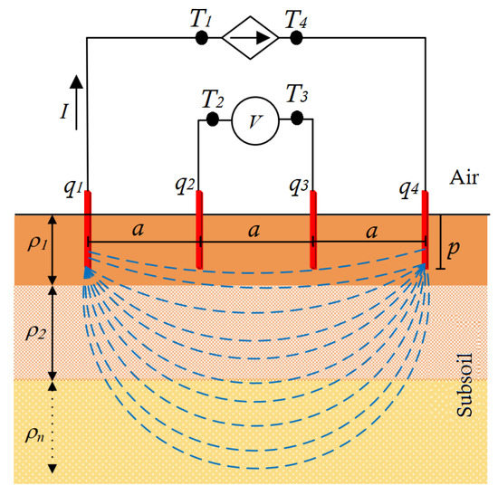
Figure 2.
Wenner’s method used to collect the soil resistivity data in field.
Several methods are applied to determine the apparent resistivity value of the soil. In an elementary way, some methodologies use the relation given by (1), where l [m] is the length and A [m is the cross sectional volume of a parallelepiped composed of a certain material. V [V] is the potential difference and I [A] is the electrical current injected in the volume extremities using electrodes, which have the same cross section of the volume.
To calculate the electrical resistivity of the soil in a noninvasive way, we need an alternative formulation to (1). This formulation is the well known geoprospecting method called Wenner’s method [35], where the apparent electrical resistivity may be given by:
where a represents the distances between two consecutive electrodes, and p is the burial depths of the electrodes, as illustrated in Figure 2. In this figure, , , and are terrometer terminals, and , , and are electrode terminals. The electrical current I is injected through terminals and , and voltage V is measured in terminals and [6].
Electrical conductivity is the intrinsic property of all conductive material of electrical current. In geoprospecting, the conductor is the soil, in which the electrical current circulates due to the presence of free salts in the soil solution (liquid phase) and also due to the exchangeable ions on the surface of the particles (solid phase). However, unlike the conductive wire, the electrical current in the ground may go through several paths, as illustrated in Figure 3, adapted from Silva Filho et al. [36]. In sufficiently moist soils, the conduction of current occurs due mainly to the salt content in the water of the soil that occupies some pores (pores with water). The solid phase may also contributes to electrical conductivity due mainly to interchangeable cations associated with clay minerals (dry soil). The third path to the electrical current in the soil occurs through soil particles with in direct and continuous contact with each other (wet soil). These three paths illustrated in Figure 3 present the current flow, which contributes to the apparent electrical conductivity of the soil [6,33,34].
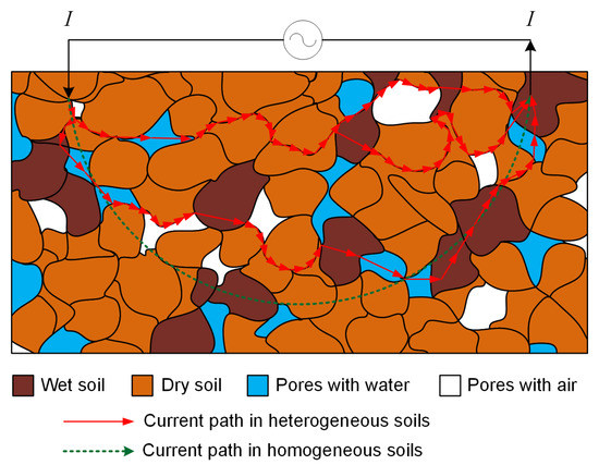
Figure 3.
Preferential path of electrical current in homogeneous and heterogeneous soil.
In Figure 2, the variable N which is subscript in and indicates the appropriate amount of layers for the stratification model to fit the studied soil. The electrical current passing through the soil from to is represented by red lines, which mostly goes through the shallow regions of the soil (58% at a depth of up to ). Since the remaining current sinks into deeper regions, this method is able to survey those depths as well. In (2), is the measured apparent resistance and if the soil is heterogeneous . Note that in (1) we include the electrical resistivity of the material, and in (2) we include the apparent resistivity. Most devices map the soil electrical conductivity by either (i) using (1) with invasive methods (which might follow erroneous procedures, as (1) is derived from electromagnetism equations, and it may only be used in homogeneous materials, which is not the case of the soil); (ii) using (2) for mapping out the apparent electrical conductivity and observing its spatial variation.
For example, two situations are presented in Figure 4, adapted from Calixto et al. [6], in which (1) would not correctly identify the structure of the soil layers for depth . The usual devices would obtain the same values of apparent electrical conductivity for both Figure 4a,b. These results would be only accurate for depth , whereas the different layers would be neglected for depth . Observe that in Figure 4b the separating surface of the second layer crosses the depth , while in Figure 4a this does not occur. This distinction between the soil layers may only be observed using 3D mapping, using (2) [6].
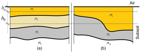
Figure 4.
Illustration where there is a need for 3D mapping: (a) any traditional mapping and (b) using 3D mapping only.
To calculate the soil electrical conductivity , after collecting the values of the soil apparent electrical resistivity , we apply a stratification method. Among the different methods for geoelectrical stratification found in the literature [2], there is a recently proposed method that minimizes the difference between the experimental and theoretical apparent resistivity curves; one of which is obtained from experimental data collected in the field, and the other is produced analytically [5]. The authors build an experimental curve of apparent resistivity utilizing Wenner’s method [37] (Figure 2), and a theoretical curve of apparent resistivity utilizing Sunde’s algorithm [38], as illustrated in Figure 5, adapted from Calixto et al. [7].
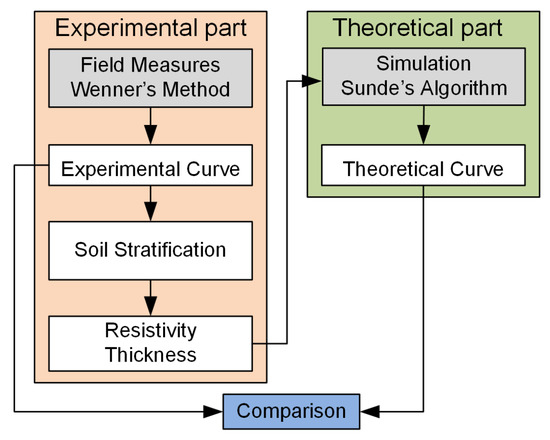
Figure 5.
Data gathering and utilization of Sunde’s algorithm.
In Figure 5 we first collect the field data using Wenner’s method, as in (2) and Figure 2, to construct an experimental curve [39]. Once the experimental curve is obtained, the soil stratification is calculated and the experimental values for the resistivities and thicknesses of each layer are found. The simulation uses Sunde’s algorithm, which takes the experimental values for the resistivities and the thicknesses of the layers as input. In the simulation, we look for the theoretical curve that is identical to the experimental curve. The theoretical curve is constructed using the values of resistivities and thicknesses of each layer and compared with the experimental curve (Figure 5). If both curves are identical, the values of resistivities and thicknesses represent the stratified soil. Otherwise, if they are not identical, the resistivity values and thicknesses of the layers are modified by the optimization process, seeking to adjust the theoretical curve to experimental one as much as possible.
2.2. Optimization Process
Sunde’s algorithm uses wave propagation equations in already stratified media to construct the theoretical resistivity curve [39]. The resistivity and thickness values are altered within the Sunde’s algorithm by using a heuristic method for optimization based on genetic algorithms. This method searches for the best solution for the stratification process and the parameters, optimized using genetic algorithm. The values optimized are: (i) the resistivity of each layer , (ii) the thickness of each layer and (iii) the number of layers N. Figure 6, adapted from Calixto et al. [7,39], shows a flowchart of the genetic algorithm.
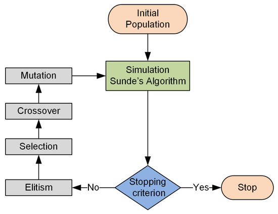
Figure 6.
Genetic algorithm flowchart.
The genetic algorithm uses an initial population formed by values of resistivity and thickness of each soil layer. Each set of parameters composed by and are used by the Sunde’s algorithm for building the theoretical curve. After simulation, each set of parameters receives a value that represents its quality as the solution of the problem. If a given set of parameters reaches the stopping criterion, the algorithm stops. Otherwise, the algorithm invokes an elitism (save the best solution) and a selection (choice of parents) process, and by the crossover (parents crossing) and mutation (mutates the new generation of possible solutions) operators, we generate a new population of possible solutions to be tested. This cycle continues until the genetic algorithm obtains an optimized solution [5,7].
3. Methodology
By applying the lateral profiling method, if the distance a between electrodes is variable represented by a vector with distinct values, the 2D mapping may lead to the 3D mapping. All process is performed in five stages: (i) discretization of area being studied; (ii) measurements using the lateral profiling method and Wenner’s method; (iii) soil stratification process; (iv) construction of 3D map; and (v) data statistical analysis.
3.1. First Stage: Discretization of Area Being Studied
This stage consists of a regular discretization of a given rectangular area to be stratified, dividing it into smaller subareas of [m], as illustrated in Figure 7. Each subarea may be defined in the L direction, by the edges and in the C direction, by the edges.
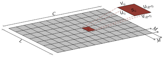
Figure 7.
Regular discretization of total area for applying 3D mapping.
3.2. Second Stage: Measurements Using Lateral Profiling Method and the Wenner’s Method
The measurements must be performed on each edge using lateral profiling method together with the Wenner’s method, where the number of edges is given by , as described in Calixto et al. [6], in which u, v and C, L must be preferably multiples of M. The arrangement of electrodes walks using the lateral profiling method, applying the Wenner’s method in all edges throughout the area to be investigated.
3.3. Third Stage: Soil Stratification Process
The stratification process is performed for each subarea using the average of values obtained from the measurements (previous stage) on each of the four edges. Thus, each subarea is stratified and the parameters are found, which are: (i) number of layers N, (ii) resistivity (or conductivity ) of each layer and (iii) thickness .
The stratification process error is given by the difference between the experimental resistivity curves and the theoretical , given by:
where k is the number of values of a and is the value that quantifies the error obtained during stratification of a subarea. Thus, the general stratification error corresponds to the sum of all values of , calculated for all subareas [6].
3.4. Fourth Stage: Construction of 3D Map
The 3D visualization of the soil being studied results from the interpolation of the thickness values of each layer related to the total area analyzed [6], in which the control points of the interpolation concern the vertices of each subarea, as shown in Figure 8. Each vertex is related to the junction of 2 or 4 subareas, except the corner vertices of the total area. Therefore, the thickness value for each vertex is the average of the thickness values obtained from stratification process for the subareas.
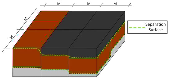
Figure 8.
Separation surface between layers of subareas.
3.5. Fifth Stage: Data Statistical Analysis
In the last stage, the global value of the resistitivity (or conductivity ) and thickness is calculated and corresponds to the mean value of the resistivity (or conductivity ) and thickness related to the all subareas. The Sample Standard Deviation (SSD) must be calculated for each global value of (or ) and . By assuming that the sample is in the universe of values of thickness , the standart deviation and (or ) quantify the dispersion of and (or ) in different subareas.
The Algorithm 1 shows all the steps of the 3D mapping flow. The main disadvantage of this methodology is the number of field measurements required. To deal with this issue, we built an automated measurement device to collect data in the field, which is used to apply the Wenner’s method automatically and to generate a 3D soil map.
| Algorithm 1: Sequence of steps of the proposed 3D mapping method. |
 |
3.6. Soil Electrical Conductivity Data Collection Device: Device Description
The Wenner’s method assumes that the current injection is punctual. This condition is satisfied in the proposed device, once that disc blade penetrates the soil down to m. In Figure 9, partial view of the device presents the assembly of the components identified by numbers.
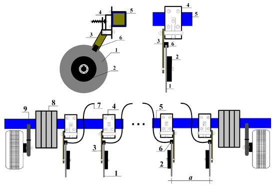
Figure 9.
Partial view of device.
The instrument proposed for automatic measuring of the soil conductivity, using the Wenner’s method, includes a set of disc blades 1 (acting as the electrodes), mounted on a transverse toolbar 5. A limiting base 2 (with a radius smaller than the discs), coupled to the disc blades, keeps the discs from penetrating the soil past a given depth. To apply the Wenner’s method, the disc blades must be arranged at a set of predefined distances a. The disc blades are connected to terminals 6 (brushes) through the disc holder 3, which in turn, are connected to cables 7 that allow injecting current and measuring the electrical potential differences.
The device may be produced in modules, i.e, given a toolbar length, one may mount any suitable number of discs, provided their number is even, and greater than 12. Wheels with tires and suspension system 9 are included in the device enabling that it is dragged by a farm vehicle. After connecting the device to the vehicle, weights 8 may be placed on the toolbar to ensure that the discs are always cutting into the soil. To provide some mechanical flexibility, the disc blades are movable in the direction of the drag, being held in place by springs 4, which allow a movement of approximately 45°. With this mechanism, the continuous contact of the discs with the soil is achieved, even if there are obstacles or irregular terrain.
3.7. Application of the Method Using the Device
The use of the device requires the suitable arrangement of the disc blades to apply the Wenner’s method. A possible disk blade configuration is shown in Figure 10 (which is out of scale), where in meters. In Figure 10, represent the conductors driven into the ground by the connected cables through which the electrical current I is injected and/or the potential difference is measured [5,6].
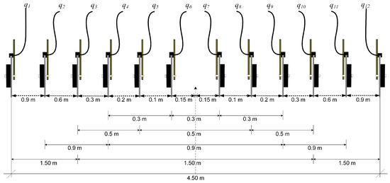
Figure 10.
Possible arrangement of disc blades.
According to Wenner’s method, when an electrical current I is injected in , coming out at , the potential difference may be measured between and . Next, the electrical resistivity meter injects the same current I in , collects it at , and measures the potential difference between and . Likewise, the same value of electrical current I is then injected in , collected at , and the potential difference between and is measured. Finally, the same current value I is injected in , collected in , and the potential difference is measured between and , completing a cycle of measurements on an edge of one subarea. It is observed that two functions are assigned to most disc blades. For instance, using the discs disposition of Figure 10, conductors and are electrical current injectors in the first moment and the same conductors and are used to measure the electrical voltage in the second moment.
If the blades distances are different from those presented in Figure 10, another distribution of the blades must be used, taking into account the distances a between the electrodes that are active during the measurements. Depending on the number of disc blades and the distances a, the toolbar will have a length equivalent to larger than the largest value of a. As the depth of the soil stratification is closely related to the distance a between disc blades, the longer the toolbar and hence the distance a, the deepest will be the stratification.
Since the device is dragged across the soil, one must specify the distance interval from one reading to the next. In accordance to the method proposed in Section 2, this distance between readings is M, however, M may assume any value above m. Hence, the subareas will always be and M is the distance that the farm vehicle moves between readings.
We need at least four values of a for the method application. If it is necessary more than four values of a to collect data, it must be added more disc blades, changing the configuration in Figure 10. The greater the vector of measures collected a, the more accurate will be the stratification of the soil. Using the configuration shown in Figure 10, a reading comprises four measurements and at each measurement, the electrical current I is injected into the ground through the terminals and of the electrical resistivity meter (Figure 11), and the voltage V is measured at the terminals and .
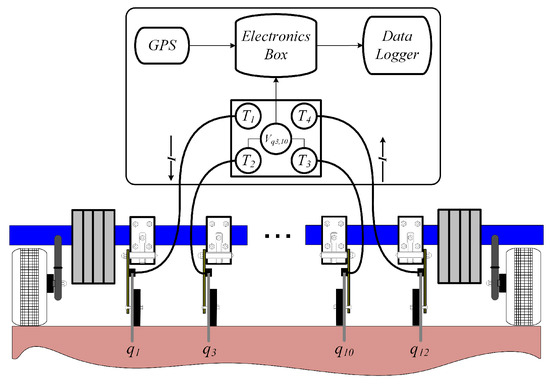
Figure 11.
Electronic system of device.
The switching of the 4 terrometer terminals in relation to the 12 electrodes is performed electronically. The Global Navigation Satellite System (GNSS) with distance-compatible precision M must provide the location of the reading, and the data are stored in the Data Logger. The data gathering is carried out when the farm vehicle is in motion and the frequency of this gathering is related to the value of M, the lower this value, the lower the speed of the farm vehicle that drags the device through the ground.
The stored data are: (i) location (latitude, longitude, and altitude) and (ii) values of the potential differences of the four measurements. If the configuration of Figure 10 is used, we have values of the potential difference for each . After performing the readings throughout the soil, the stored data are placed on the computer for processing. After the treatment of data, the stratification and the 3D mapping of the soil are generated. Figure 12 illustrates the whole flow of methodology for using the proposed device.
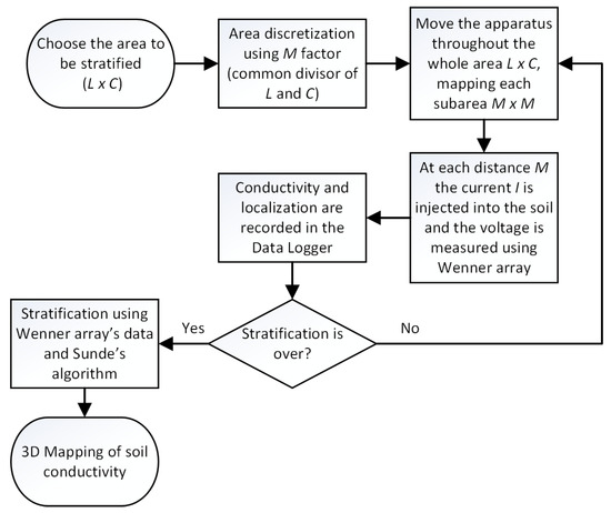
Figure 12.
Flowchart for use of proposed methodology and device.
4. Results
In this section, we present the results obtained when the proposed method is applied. These results refer to the efficacy of the method: (i) to identify soil differences under controlled conditions, (ii) to perform soil stratification, and (iii) to perform 3D soil mapping.
4.1. 2D Mapping with Modifications Provoked in the Soil under Controlled Conditions
In this study, two experiments were carried out to validate the method: (i) the soil moisture analysis and (ii) the soil compaction analysis. The experiments were carried out in an open area with low humidity, hence the soil was relatively dry, located at 16°30170 S and 49°16530 W at an altitude of 819.20 m. To limitate the region to be studied and place the rods, ropes were attached to wood stakes with a limited area of 5 m × 5 m, the spacing between the rods was 1 m, and the depth of the rods was m. Figure 13 presents the area limitation geometry for applying the lateral profiling method and obtaining the data.
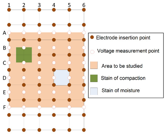
Figure 13.
Definition of area and application of method.
4.1.1. Soil Moisture Study
In the area limited by ropes, a quadrant was chosen to insert approximately eight liters of water to change the dynamics of the system. Figure 14a shows the connectors/rods with the cables, where the red arrows indicate the electrical current cables and the green arrows indicate the voltage cables. In Figure 14b, it may be observed the spot where the portion of water in the soil was spilled.
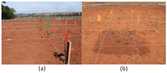
Figure 14.
Preparation of area for application of lateral profiling method: (a) insertion of electrodes and (b) area with insertion of water.
To evaluate the method, the electrical resistance measurement is performed in the study area before and after the insertion of the water portion. Table 1 provides the values of the electrical resistance measured using the terrometer, where and are the electrical resistances before and after insertion of the water portion, respectively. These electrical resistance values were measured along Line A through Line F and along Column 1 through Column 6.

Table 1.
Electrical soil resistance values under controlled conditions for soil water content mapping.
From the data of Table 1 and from (2), it is possible to map the dynamics in the soil due to the water insertion. Figure 15a presents the result of the distribution of apparent electrical conductivity related to the soil at the initial conditions (without water insertion), Figure 15b presents the distribution of apparent electrical conductivity related to the soil after the water insertion and Figure 15c presents the subtraction of the values obtained with and without water insertion.
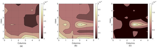
Figure 15.
2D mapping of electrical conductivity due to insertion of water in soil: (a) before, (b) after, and (c) difference between after and before.
Figure 15c presents the dynamics in the soil due the water insertion and identifies the position where the change occurred. To validate the experiment and compare the obtained results, a Time Domain Reflectometer (TDR) is used in the same area, before and after the insertion of water. The results obtained are presented in Table 2 and in Figure 16, where Figure 16a presents the result of the moisture distribution related to the soil at the initial conditions (without water insertion), Figure 16b presents the moisture distribution related to the soil after the water insertion, and Figure 15c presents the subtraction of the values obtained with and without water insertion .
Table 2.
Soil moisture values under controlled conditions.
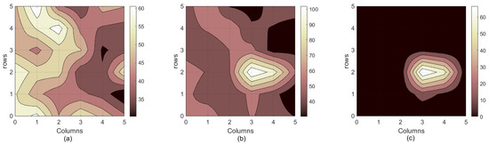
Figure 16.
2D mapping of moisture dynamics in soil: (a) , (b) and (c) .
4.1.2. Study of Soil Compaction
The methodology presented in Figure 13 is also used to measure the soil compaction level dynamics and to validate the proposed method. This experiment was conducted in other area 20 m away from the previous experiment area. In this experiment, the level of soil compaction was changed in the region shown in Figure 13 due to the impacts produced using a metal object of to compress the soil corresponding to area of 1 m × 1 m. Table 3 presents the values of electrical resistance obtained before and after the soil compaction and Figure 17 presents the distribution of the apparent resistivity values.
Table 3.
Electrical resistance values of soil under controlled conditions for mapping level of soil compaction.
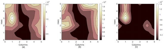
Figure 17.
2D mapping of electrical resistivity due to changes in soil compaction: (a) before, (b) after, and (c) difference between after and before.
In Figure 17a the distribution of apparent resistivity before the soil compaction is presented, in Figure 17b the distribution of apparent resistivity after the soil compaction is presented, and Figure 17c has the value of the difference between after and before the soil compaction. To validate the data obtained by the proposed method application, a digital penetrometer is used to carry out measurements of the compaction levels at the same area. This procedure is also performed before and after soil compaction, to verify the soil resistance to penetration. Table 4 presents data obtained using digital penetrometer, in which is the soil compaction before the change in the structure and is the soil compaction after the change made with the metal object, both measured in .
Table 4.
Soil compaction values and under controlled conditions.
From Table 4, it is possible to construct the distribution map of the compaction levels before and after the change in soil structure. Figure 18a presents the level of compaction prior to the change in soil structure, Figure 18b presents the level of compaction after the change in the structure of the soil, and Figure 18c presents the dynamics occurred in the soil structure due to changes in soil compaction level, .
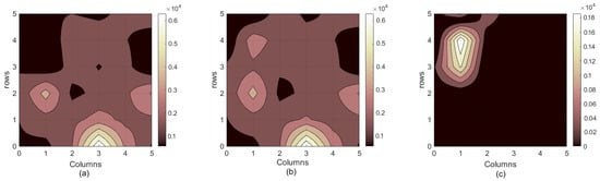
Figure 18.
2D mapping of soil compaction dynamics: (a) , (b) and (c) .
Two-dimensional mappings were performed in Section 4.1, in which the value of a was kept constant in 1 m. The depth analyzed was m, considering the whole soil as uniform in the space or . All studies were performed manually. However, to map the soil bidimensionally using the proposed device, simply place all disc blades of current injection with the same distance a constant and perform the multiplexing in the data reading of the electrodes. Thus, there is no need to perform horizontal stratification of the soil, since for a constant and the measured values are directly mapped using (2).
4.2. 3D Mapping with Soil Classification
The 3D mapping was performed based on lateral profiling method in conjunction with measurements of the apparent electrical resistivity for several values of a. In the stratification process, it is necessary to construct the curves and . The next studies use the proposed methodology to consctruct the 3D mapping of the soil with and , M and a in meters. In addition to the application of the method, a trench was opened at the edge of each area being studied to identify and classify pedogenic horizons and soil layers.
To interpret the results presented in the tables in this section, one must be aware of the difference between pedogenetic horizon and soil layer. By definition, the pedogenetic horizon is a soil section approximately parallel to the soil surface, whose characteristics are inherited by weathering conditions [40], and it is related to different characteristics of the soil such as its chemical composition, texture, color, porosity, and percentage of organic material and/or minerals.
On the other hand, a soil layer is a soil section with particular organic or mineral formation, approximately parallel to the soil surface, whose properties do not result from the pedogenetic processes (or with low influence) [8]. Soil layers are used in geoprospection, taking into consideration the variation of the soil electrical conductivity .
4.2.1. Profile of the Plinthosol
This study was conducted at 14°23625 S and 47°03804 W coordinates, at an altitude of 432 m. The parental material of this soil are tertiary and quaternary sediments originated from Arkoses and pelites of the Three Mary formation from the Bambuí Group (Neoproterozoic).
This profile (Figure 19) was described and classified by SiBCS as a Argilluvic Plinthosols concretionary dystrophice and as a Typic Plinthaquox by the Soil Taxonomy. In Table 5, the sequence of the pedogenetics horizons is listed. Figure 20 presents an interpolated view of the soil mapping, and the colorbar represents the depth of the separation surface between the layers with the thicknesses and .
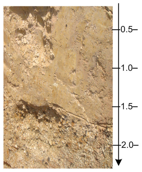
Figure 19.
Profile of Plinthosol.
Table 5.
Pedogenetics horizons of Plinthosol.
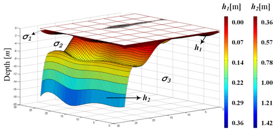
Figure 20.
View of 3D mapping for profile of Plinthosol.
This is a soil with low hydraulic drainage, which may be attributed to the occurrence of plinthite and petroplinthite in horizon (plinthite and concretions). This soil belongs to flat relief. In this study, the number of sites where the readings were collected was , resulting in 36 subareas. Table 6 presents the global values of the conductivities together with the thickness and its sample standard deviations.
Table 6.
Mean values and sample standard deviations of 3D mapping of Plinthosol.
In Table 5, the interval between horizon and horizon belongs to the first layer of the soil, while the horizons E, e belong to the second layer, according to Table 6. The approximate mineralogical [41] in the several granulometric fractions on the Plinthic horizon () of this soil is composed by: (i) clay () Kaolinite (dominant), with inclusions of gibbsite, mica, and smectite; (ii) gravels, nodules, ferruginous concretions, and concretionary fragments (Petroplinthite) that restrict permeability and free drainage; (iii) coarse sand, of ferruginous concretions and concretionary fragments (Petroplinthite) and of quartz + hyaline quartzite; and (iv) thin sand, of quartz, and even of ferruginous concretions. The high values obtained for the conductivity are associated with high humidity of this soil. This high humidity, associated with the presence of a material rich in iron oxide, with ferruginous concretion concentrations and associated with quartzite that contains of magnesium, results in a good electrical conductivity of the soil.
4.2.2. Profile of the Leptosol
This study was performed at the coordinates 12°5838.5 S and 46°5401.0 W, with an altitude of 613 m. The parental material of this soil is composed of micaceous quartzite and feldspathic Araí Group (Neoproterozoic). The soil profile (Figure 21) was described and classified by the Brazilian System of Soil Classification (SiBCS) [42] as an Udorthent Dystrophic leptic, epialic, kaolinitic, medium-subdeciduos tropical Cerrado phase, and strongly undulated relief, and it was classified by the Soil Taxonomy as a Lithic Orthents [40].
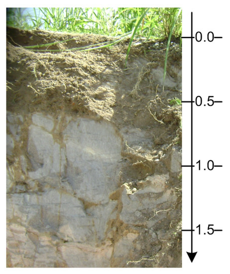
Figure 21.
Profile of the Leptosol.
The sequence of the pedogenetic horizons is presented in Table 7. The macroscopic analysis of the samples revealed two different types of rocks: (i) quartzite interwoven with thin clay layers (ii) metassiltites with poorly developed schistosity, interspersed with quartz and feldspar. In terms of chemical elements, the rocks and some soils are characterized by their poverty in nutrients, with saturation by basic cations in the order of in the horizon A and approximately in the subhorizon .
Table 7.
Pedogenetic horizons of Leptosol.
In this study, the number of sites where the readings were performed was , resulting in 36 subareas. Figure 22 presents an interpolated viewing of this soil mapping, and the colorbar represents the depth of the separation surface between the layers with thicknesses and .
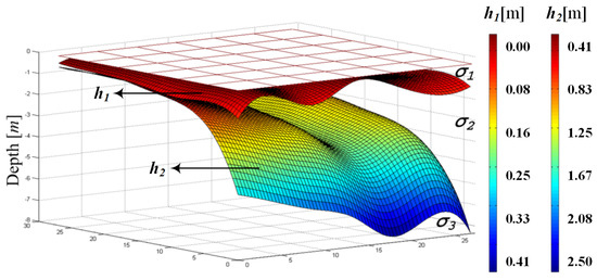
Figure 22.
View of 3D mapping for profile of Leptosol.
This study analyzed extremely weak soil for agricultural purposes, indicated only for environmental preservation, although it was deforested for using as pasture. Table 8 presents the global values of the conductivities together with their thickness and the sample standard deviations and . Table 7 presents that the interval between horizon A, and horizon belongs to the first layer of the soil, according to Table 8, while horizon belongs to the second layer . The low conductivity of this soil is due to the low saturation of basic cations. The approximate mineralogical formation in the various granulometric fractions of the horizon is composed of: (i) clay (): Kaolinite (dominant), with inclusions of mica (muscovite); (ii) coarse sand: ; (iii) thin sand: even of quartz and quartzite [41].
Table 8.
Mean values and sample standard deviations of 3D mapping of Leptosol.
4.2.3. Profile of the Nitisol
This study was conducted at 14°14456 S and 47°03328 W coordinates, at an altitude of 458 m with a local and regional plain relief, phase Tropical deciduous Forest. A profile section of this soil is illustrated in Figure 23. The pedogenetic horizon distributions follow the description presented in Table 9.
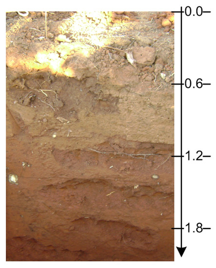
Figure 23.
Profile of Nitisol.
Table 9.
Pedogenetic horizons of the Nitisol.
The soil parental material is limestone of the Alligator Pond Formation from Bambuí Group (Neoproterozoic), with low degree of metamorphism. The soil is classified by the SiBCS as an Alfisol Eutrophic Argisolic and by the Soil Taxonomy as a Typic Haplustult. Figure 24 presents an interpolated view of the soil mapping, and the colorbar represents the depth of the separation surface between the layers with the thicknesses and .
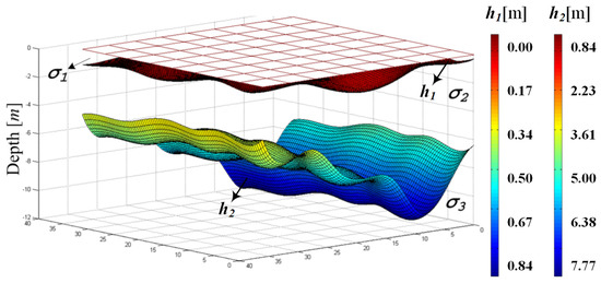
Figure 24.
View of 3D mapping for profile of Nitisol.
The mineralogy, in accordance to Dixon & Schulze [41], has a closer composition in its respective fractions of the horizon , containing: (i) clay () predominantly kaolinite; (ii) gravel, nodules or spherical ferruginous concretions, fragments of weathered rock (phyllite type), white-hyaline quartz and traces of carbonate material; (iii) coarse sand, of nodules or spherical ferruginous concretions of quartz + quartzite, white-hyaline, with ferruginous encrustations; (iv) fine sand, hyaline-white quartz, milky, with ferruginous incrustation, of ferruginous concretions coal + debris. In this study, the number of sites where the readings were collected was , resulting in 64 subareas.
Table 10 presents the global values of the conductivities together with the thickness and the sample standard deviations e . In Table 9 and Table 10, note that the pedogenetic horizons A, and belongs to layer and only the horizon belongs to the second layer of the soil. In layers and , the high values of the electrical conductivity are related to the elevated content of clay in the horizon , approximately higher than in the diagnostic horizon A Chernozemic. In horizon A, high contents of calcium and carbon were found. In layer , there was high content of basic cations, leading to low value of electrical conductivity.
Table 10.
Mean values and sample standard deviations of 3D mapping of Nitisol.
In this study, the concentration of basic cations in depth occurs because we are in a region where the rainfall is sufficient to leach basic cations to the layer . Hence, the cations removed from the two superior layers are replaced by hydrogen and aluminum from the weathering minerals. Acidification of layers and occurs by a natural process, leading them to become more electrically conductive.
4.3. Discussion
In the Section 4.1, Table 1 and Table 2 exhibit the values obtained before and after the soil modifications: (i) chemical (water insertion) and (ii) physical (compaction). The values presented demonstrate the sensitivity of the method for soil dynamics analysis, proving its efficiency in the monitoring of the subsoil structure. It is further observed from Table 1 and Table 2 that the proposed method is more sensitive to variations than TDR and penetrometer. This fact is due to other factors that may be measured using the proposed method, such as plant roots, and stones and voids in the soil, among others.
In the Section 4.2, 3D mappings are performed. In addition to the visualization form presented in Figure 20, Figure 22 and Figure 24, there are other forms of visualizing the 3D mapping, such as the mapping of the separating surfaces between layers, using the values of without any interpolation, i.e., representing the stratification performed on each subarea. Figure 25 presents this kind of visualization for the mapping of the profile of the Leptosol, with the colorbar representing the depth of the separation surface between the layers of each subarea with the thicknesses and .
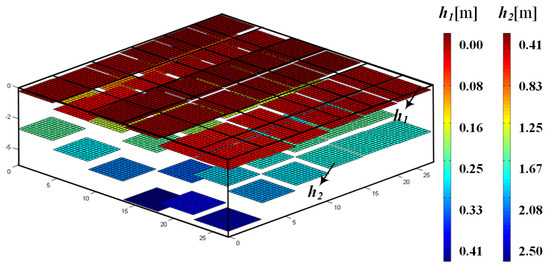
Figure 25.
Visualization of mapping without interpolation of Leptosol’s profile.
Table 6, Table 8 and Table 10 present mean values of electrical conductivity and thickness ( and ) that vary throughout the soils being studied. The SSD is small for the electrical conductivity values, with maximum of . However, the values of the standard deviation of the thicknesses are higher, reaching due to the amount of subareas, leading to several stratifications. Thus, using the values obtained from the stratifications of each subarea, it is possible to produce the all subareas mapping in each layer instead of producing the area mapping as whole. This mapping originates from the horizontal stratification of the soil and not from the lateral profiling method. The map translates the processed data as a visualization of the conductivities distributed over the soil surface. In the proposed method, this view may be obtained for each layer. An example of this visualization is illustrated in Figure 26, whereas the colormap is the same as for Figure 27 and each value is presented in mS.m.
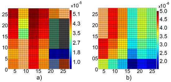
Figure 26.
Visualization of a subarea’s conductivities in Leptosol’s profile. (a) First layer and (b) second layer.
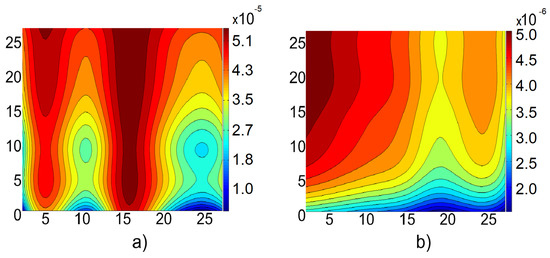
Figure 27.
Isovalues curves of Leptosol’s profile. (a) First layer. (b) Second layer.
In Figure 26, it is possible to observe the variation of the electrical conductivity through the 2D mapping of the isovalue curves. These curves may be mapped to each soil layer, where each color represents a range of conductivity values. In Figure 27, presents a view of the conductivity variation of the profile of Leptosol for the first and second layers. In this case 15 range values of conductivity were considered in each layer. As in Figure 25, Figure 26 and Figure 27 may only be obtained from the stratification process.
The proposed method allows to determine in which depth a certain conductivity value may be found, from a statistical treatment of the data obtained from the stratification of several areas. Table 11 lists some statistic data, referred to the layers depth of several subareas, from which Figure 28 may be produced. In Table 11 and Figure 28, is the inferior surface depth of each layer i (the points where layer i ends and layer begins), given by (4). The last layer assumes an infinite depth, since its thickness is also infinite, in accordance with the adopted model.
Table 11.
Depth values (mean, minimum, maximum, and standard deviation) until limitation of several layers.
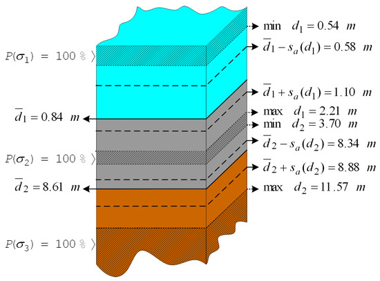
Figure 28.
Depth layers distribution.
Table 11 and Figure 28 show that for the stratified soil of profile of the Nitisol, the first layer reaches at least a depth of m (min ) in the entirely terrain extension. Likewise, any point in the interval between m (max ) and m (min ) will be in the second layer. Above the depth value of m (max ), there is only third layer (in all the terrain). In Figure 28 the hatched depths are those in which a given layer is found (with its respective conductivity) with a probability of (i.e., at such depth there is the predominance of only one layer in all the terrain).
Considering that the thickness values of the layers correspond to the normal Gaussian distribution, the data presented in the Table 11 and in Figure 28 may be described in the form of the Table 12, presenting the probability of finding given layer i at depth d. For instance, at a depth of () the probability of still being in the first layer is only , and to already be in the second layer is .
Table 12.
Probability of finding layer at depth d.
All the studies presented earlier were chosen to validate the proposed methodology. Therefore, the stratifications with mineral composition analysis and the location of the studied region were performed only to present to the reader some basic characteristics of the different soils, such as the study of profile of the Leptosol (Figure 21), which has as a characteristic a superficial layer of crop land soil of small thickness and layers of rocks below the cultivable soil layer. Presenting and discussing the mineral compositions of the studied soils is outside the scope of this research.
In the studies in which the 3D mapping was carried out, high computational effort was demanded. The optimization process consumes on average three minutes to stratify each edge of each subarea. After the stratification process, the computational manipulation of the data spends approximately four minutes to generate the maps related to the 3D mapping; for example, for the profile of the Leptosol: Figure 22 and Figure 25, Figure 26 and Figure 27.
Regarding the use of the apparatus on nonplanar surfaces, the level of roughness must be observed. It is possible to use the proposed methodology on these surfaces as long as the surface roughness is less than the length of the apparatus. The proposed methodology used the shortest possible length so that the Wenner array could be used.
When using the proposed methodology together with the apparatus that is being dragged over the ground, it may occur that elements such as pieces of wood, among others, cause the noninsertion of all electrodes in the ground. Thus, when collecting the values of the apparent electrical resistivity of the soil, if the electrodes are not all connected to the ground, the terrometer informs with an audible signal so that the farm vehicle operator can analyze and make the most satisfactory decision. The terrometer used in this work, in addition to indicating the nonconnection of all electrodes, also accounts for spurious currents.
5. Conclusions
The application of the Wenner’s method in conjunction with the lateral profiling method leads to the construction of 3D soil maps. The use of more accurate methods of measuring soil electrical conductivity reduces the number of required physical and chemical analyzes. The 3D mapping of soil electrical conductivity may be correlated with physical, chemical, and biological attributes of the soil, providing information on the distribution of such attributes and indicating where to apply the agricultural inputs accurately.
The device presented in this paper contributes to obtaining maps similar to those obtained by means of computed tomography, identifying regions of the same characteristics from 3D approach. The identification of the layers distribution (in depth) facilitates the application of agricultural inputs according to the root system of the crops, besides being useful in researches about hydrodynamic and soil compaction. The proposed device still solve the problem of the large number of measurements needed when the proposed methodology is applied.
The device for collection of field data may be used to measure the apparent soil electrical conductivity on a large scale automatically, with a sufficient amount of measures to produce a stratification. The 3D mapping is more accurate than the simple mapping of apparent conductivity, even when these are performed at large depths, enabling the correct identification of the soil structure.
The measurements of the soil apparent conductivity used in the stratification method described were performed manually by fixing electrodes in the soil. The proposed device is still in a prototype phase. The depth to be stratified is directly related to the width of the device. Given that the root system of some plants may reach depths in the order of 4 m, it is recommended a m-wide device, which may be inconvenient to handle.
The proposed method enables a 3D structure description of a complex soil, being useful in the agricultural field, identifying layers in cultivable soils and describing their heterogeneity. The proposed device is the appropriate tool for the 3D mapping of soil electrical conductivity.
6. Patents
Author Contributions
W.P.C. developed the mathematical modeling. W.P.C., C.L.B.S., A.M.S.F. and M.R.C.R. built the prototype for soil data collection. W.P.C., C.L.B.S., A.M.S.F. and V.M.G. applied the methodology and conducted the experiment in loco. W.P.C., G.A.W., A.M.S.F. and M.R.C.R. analyzed and treated the data collected. W.P.C., C.L.B.S., V.M.G., M.R.C.R., A.M.S.F., A.P.C., G.A.W. analyzed the results and collaborated writing the
manuscript. All authors have read and agreed to the published version of the manuscript.
Funding
This research received no external funding.
Data Availability Statement
Not applicable.
Acknowledgments
The authors would like to thank National Council for Scientific and Technological Development (CNPq), Foundation for Research Support of the State of Goias (FAPEG) and Brazilian Federal Agency for Support and Evaluation of Graduate Education (CAPES) for scholarships: 88881.133454/2016-01 and 88881.132192/2016-01. The authors also thank CAPES for funding the studies in the Sanduiche period carried out by student Carlos Leandro Borges da Silva at the University of South Florida.
Conflicts of Interest
The authors declare no conflict of interest.
References
- Tabbagh, A.; Dabas, M.; Hesse, A.; Panissod, C. Soil resistivity: A Non-invasive Tool to Map Soil Structure Horizontal. Geoderma 2000, 97, 393–404. [Google Scholar] [CrossRef]
- Griffiths, D.H.; King, R.F. Applied Geophysics for Engineers and Geologists: The Elements of Geophysical Prospecting; Pergamon Press: Oxford, UK, 1981. [Google Scholar]
- Srinivasan, A. Handbook of Precision Agriculture. Principles and Applications; The Haworth Press Inc.: New York, NY, USA, 2006. [Google Scholar]
- Pendergrass, A.G.; Knutti, R.; Lehner, F.; Deser, C.; Sanderson, B.M. Precipitation Variability Increases in a Warmer Climate. Sci. Rep. 2017, 7, 10799. [Google Scholar] [CrossRef] [PubMed]
- Calixto, W.P.; Martins Neto, L.; Wu, M.; Kliemann, H.J.; Castro, S.S.; Yamanaka, K. Calculation of Soil Electrical Conductivity Using a Genetic Algorithm. Comput. Electron. Agric. 2010, 71, 1–6. [Google Scholar] [CrossRef]
- Calixto, W.P.; Nobre, F.S.; Alves, A.J.; Domingues, E.G.; Domingos, J.L.; Pires, T.G.; Ferraz, R.S.; Gomes, V.M. Methodology for 3D mapping soil electrical conductivity: A case study. In Proceedings of the Conference on Electrical, Electronics Engineering, Information and Communication Technologies, Santiago, Chile, 28–30 October 2015. [Google Scholar]
- Calixto, W.P.; Martins Neto, L.; Wu, M.; Yamanaka, K. Parameters Estimation of a Horizontal Multilayer Soil Using Genetic Algorithm. IEEE Trans. Power Deliv. 2010, 25, 1250–1257. [Google Scholar] [CrossRef]
- EMBRAPA. Criteria for Differention of Soil Types and Stages of Mapping Units: Standards in Use by SNLCS; National Service of Soil Survey and Conservation—SNLCS: Rio de Janeiro, Brazil, 1988. (In Portuguese) [Google Scholar]
- Luck, E.; Eisenreich, M. Electrical Conductivity Mapping for Precision Agriculture. In European Conference on Precision Agriculture; Ecole National Supériure Agronomique: Montpellier, France, 2001. [Google Scholar]
- Maxbauer, D.P.; Feinberg, J.M.; Fox, D.L.; Nater, E.A. Response of pedogenic magnetite to changing vegetation in soils developed under uniform climate, topography, and parent material. Sci. Rep. 2017, 7, 17575. [Google Scholar] [CrossRef]
- Corwin, D.L.; Lesch, S.M. Application of Soil Electrical Conductivity to Precision Agriculture: Theory, Principles and Guidelines. Agron. J. 2003, 95, 455–470. [Google Scholar] [CrossRef]
- Loke, M.H.; Chambers, J.E.; Rucker, D.F.; Kuras, O.; Wilkinson, P.B. Recent developments in the direct-current geoelectrical imaging method. J. Appl. Geophys. 2013, 95, 135–156. [Google Scholar] [CrossRef]
- Lund, E.D.; Christy, C.D.; Drummond, P.E. Applying Soil Electrical Conductivity Technology to Precision Agricultur. In Proceedings of the 4th International Conference on Precision Agriculture, St. Paul, MN, USA, 19–22 July 1998. [Google Scholar]
- Coelho, E.F.; Or, D. Root Distribution and Water Uptake Patterns of Corn Under Surface and Subsurface Drip Irrigation. Plant Soil Dordr. 1999, 206, 123–136. [Google Scholar]
- FAO. The State of Food and Agriculture. In David Lubin Memorial Library Cataloguing in Publication Data; FAO: Rome, Italy, 1998. [Google Scholar]
- Silva, S.; Whitford, W.G.; Jarrell, W.M.; Virginia, R.A. The Microarthropod Fauna associated with a Deep Rooted Legume, Prosopis Glandulosa, in the Chihuahuan Desert. Biol. Fertil. Soils 1989, 7, 330–335. [Google Scholar] [CrossRef]
- Gebbers, R.; Luck, E.; Dabas, M.; Domsch, H.A. Comparison of instruments for geoelectrical soil mapping at the field scale. Near Surf. Geophys. 2009, 7, 179–190. [Google Scholar] [CrossRef]
- Canadell, J.; Jackson, R.B.; Ehleringer, J.R.; Mooney, H.A.; Sala, O.E.; Schulze, E.D. Maximum Rooting Depth of Vegetation Types at the Global Scale. Oecologia 1996, 108, 583–595. [Google Scholar] [CrossRef] [PubMed]
- Bohm, W. Methods of Studying Root Systems; Series: Ecological Studies v. 33; Springer: Berlin/Heidelberg, Germany, 1979. [Google Scholar]
- Bassoi, L.H.; Fante Junior, L.; Jorge, L.A. C; Crestana, S.; Reichardt, K. Distribution of Maize Root System in a Kanduidalfic Eutrudox Soil: II. Comparison between Irrigated and Fertirrigated Crops. Sci. Agrícola 1994, 51, 541–548. [Google Scholar] [CrossRef]
- McCulley, R.; Jobbágy, E.; Pockman, W.; Jackson, R. Nutrient Uptake as a Contributing Explanation for Deep Rooting in Arid and Semi-arid Ecosystems. Oecologia 2004, 141, 620–628. [Google Scholar] [CrossRef] [PubMed]
- Wiersum, L.K. Potential Subsoil Utilization by Roots. Plant Soil 1967, 27, 383–400. [Google Scholar] [CrossRef]
- Fox, R.L.; Lipps, R.C. Distribution and Activity of Roots in Relation to Soil Properties; Seventh International Congress of Soil Science: Madison, WI, USA, 1960; pp. 260–267. [Google Scholar]
- Seger, M.; Cousin, I.; Frison, A.; Boizard, H.; Richard, G. Characterization of the structural heterogeneity of the soil tilled layer by using in situ 2-D and 3-D electrical resistivity measurements. Soil Tillage Res. 2009, 103, 387–398. [Google Scholar] [CrossRef]
- Besson, A.; Cousin, I.; Samouelian, A.; Boizard, H.; Richard, G. Structural Heterogeneity of the tilled layer as Characterized by 2D electrical resistivity Surveying. Soil Tillage Res. 2004, 79, 239–249. [Google Scholar] [CrossRef]
- Samouelian, A.; Cousin, I.; Tabbagh, A.; Bruand, A.; Richard, G. Applied Geophysics. Soil Tillage Res. 2005, 83, 173–193. [Google Scholar]
- Telford, W.M.; Geldart, J.L.; Sheriff, R.E.; Keys, D.A. Applied Geophysics, 2nd ed.; Cambridge University Press: Cambridge, UK, 1976; pp. 62–596. [Google Scholar]
- Petrovic, A.M.; Siebert, J.E.; Rieke, P.E. Soil bulk density analysis in three dimensions by computed tomographic scanning. Soil Sci. Soc. Am. J. 1982, 46, 445–463. [Google Scholar] [CrossRef]
- Crestana, S.; Mascarenhas, S.; Pozzi-mucelli, R.S. Static and dynamic 3D studies of water in soil using computerized tomography scanning. Soil Sci. 1985, 140, 326–347. [Google Scholar] [CrossRef]
- Balogun, F.A.; Cruvinel, P.E. Compton scattering tomography in soil compaction study. Nucl. Instrum. Methods Phys. Res. 2003, 505, 502–530. [Google Scholar] [CrossRef]
- Pires, L.F.; Macedo, J.R.; Souza, M.D.; Bacchi, O.O.S.; Reichardt, K. Gamma-ray computed tomography to investigate compaction on sewage-sludge-treated soil. Appl. Radiat. Isot. 2003, 59, 17–43. [Google Scholar] [CrossRef]
- Silva Filho, A.M.; Calixto, W.P.; Alves, A.J.; Silva, J.R.S.; Fernandes, G.M.; Morais, L.D.S.; Coimbra, A.P. Root System Analysis and Influence of Moisture on Soil Electrical Properties. Energies 2021, 14, 6951. [Google Scholar] [CrossRef]
- Silva Filho, A.M.; Furriel, G.P.; Calixto, W.P.; Alves, A.J.; Profeta, F.A.; Domingos, J.L.; Domingues, E.G.; Narciso, M.G. Methodology to Correlate the Humidity, Compaction and Soil Apparent Electrical Conductivity. In Proceedings of the Conference on Electrical, Electronics Engineering, Information and Communication Technologies, Santiago, Chile, 28–30 October 2015. [Google Scholar]
- Silva Filho, A.M.; Silva, C.L.B.; Assfalk, M.A.O.; Gumeratto, T.P.; Alves, A.J.; Calixto, W.P.; Narciso, M.G. Correlation method of physical characteristics with electrical properties of the soil. In Proceedings of the Conference on Electrical, Electronics Engineering, Information and Communication Technologies, Santiago, Chile, 22–24 September 2016. [Google Scholar]
- Orellana, E. Geoelectrical Prospection in Direct Current; Biblioteca Tecnica Philips: Madrid, Spain, 1974. (In Spanish) [Google Scholar]
- Silva Filho, A.M.; Calixto, W.P.; Alves, A.J.; Silva, C.L.B.; Pires, T.G.; Oliveira, A.A.; Alves, A.J.; Narciso, M.G. Geoelectric method applied in correlation between physical characteristics and electrical properties of the soil. Trans. Environ. Electr. Eng. 2017, 2, 37–44. [Google Scholar] [CrossRef]
- Wenner, F.A. Method of Measuring Earth Resistivity; Bulletin of the National Bureau of Standards: Washington, DC, USA, 1916; Volume 12. [Google Scholar]
- Sunde, E.D. Earth Conduction Effects in Transmission Systems; MacMilan: New York, NY, USA, 1968. [Google Scholar]
- Calixto, W.P.; Coimbra, A.P.; Alvarenga, B.; Molin, J.P.; Cardoso, A.; Neto, L.M. 3D Soil Stratification Methodology for Geoelectrical Prospection. IEEE Trans. Power Deliv. 2012, 27, 1636–1643. [Google Scholar] [CrossRef]
- Soil Survey Staff. Soil Taxonomy: A Basic System of Soil Classification for Making and Interpreting Soil Surveys; U.S. Government Printing Office: Washington, DC, USA, 1999. [Google Scholar]
- Dixon, J.B.; Schulze, D.G. Soil Mineralogy with Environmental Applications; Soil Science Society of America Inc.: Madison, WI, USA, 2002. [Google Scholar]
- EMBRAPA. Brazilian Soil Classification System—SiBCS; Embrapa-SPI: Rio de Janeiro, Brazil, 2006. [Google Scholar]


Publisher’s Note: MDPI stays neutral with regard to jurisdictional claims in published maps and institutional affiliations. |
© 2022 by the authors. Licensee MDPI, Basel, Switzerland. This article is an open access article distributed under the terms and conditions of the Creative Commons Attribution (CC BY) license (https://creativecommons.org/licenses/by/4.0/).