Abstract
An increase in air temperature leads to a significant transformation of the relief and landscapes of the Arctic. The rate of permafrost degradation, posing a profound change in the Arctic landscape, depends on air temperature, vegetation cover, type of soils, surface and ground waters. The existing international circumpolar programs dedicated to monitoring the temperature state of permafrost TSP (Thermal State Permafrost) and active layer thickness CALM (Circumpolar Active Layer Monitoring) are not sufficient for a comprehensive characterization of geocryological conditions. Yet, no standardized protocol exists for permafrost monitoring and related processes. Here, we propose a novel multi-parameter monitoring protocol and implement it for two sites in the European part of the Russian Arctic: the Yary site along the coast of the Baydaratskaya Bay in the Kara Sea (68.9° N) within the continuous permafrost area and the Hanovey site in the Komi Republic (67.3° N) within the discontinuous permafrost area. The protocol includes drilling boreholes, determining the composition and properties (vegetation cover and soils), snow cover measurement, geophysical imaging, active layer estimation and continuous ground temperature measurements. Ground temperature measured in 2014–2020 revealed that amplitudes of surface temperature fluctuations had no significant differences between the Yary and Hanovey sites, while that the mean annual temperatures between the areas had a considerable difference of greater than 3.0 °C. The period of the presence of the active layer changed with the year (e.g., ranging between 135 and 174 days in the Yary site), showing longer when the air temperatures in summer and the preceding winter were higher. Electrical resistivity tomography (ERT) allowed determining the permafrost distribution and active layer thicknesses. Thermometry results were consistent with our geophysical data. Analyzing the composition and properties of frozen soils helped better interpret the data of geophysical and temperature measurements. By integrating the study of the soil properties, ground temperatures, and ERT, our work allowed us to fully characterize these sites, suggesting that it helps better understand the thermal state at any other research sites in the European north of Russia. Our suggested monitoring protocol enables calibrating and verifying the numerical and analytical models of the heat transfer through the earth’s surface.
1. Introduction
Permafrost covers 21 million km2, accounting for 22% of the exposed land area in the Northern Hemisphere [1]. The distribution and characteristics of permafrost are not uniform. They are influenced by various factors, including air temperature, snow and vegetation covers, geomorphological position, and soil properties [2]. The evaluation of each parameter should be in the monitoring protocol. Over the past few decades, the polar and high-altitude regions have warmed faster than elsewhere, leading to permafrost warming (ground temperature increased by 0.39 ± 0.15 °C over the past decade [3,4]) and thawing. Permafrost degradation due to climate change impacts the local environment [5], Arctic people [6,7], and infrastructure [8,9,10]. In addition, permafrost thawing can encourage global warming via the emission of greenhouse gases [11,12].
The permafrost monitoring is available at different spatial levels: global, national, regional, and local levels. However, protocols of observations in different levels should be grounded in a single methodological basis. At the global level, the World Meteorological Organization (WMO) and International Permafrost Association (IPA), including Global Terrestrial Network for Permafrost (GTN-P) and Circumpolar Active Layer Monitoring (CALM) programs, provide some protocols [13,14,15,16]. A national permafrost monitoring network is provided in Norway (Thermal State of Permafrost in Norway and Svalbard) and Switzerland (Swiss Permafrost Monitoring Network). An integrated earth systems science framework on diverse aspects related to thawing permafrost conditions in the Canadian Arctic will develop according to the Arctic Development and Adaptation to Permafrost in Transition program [17]. The Russian national permafrost monitoring system will start in 2023 according to the Decree of Russian Federation President No. 204 “On the national goals and strategic objectives of the development of the Russian Federation for the period until 2024” (7 May 2018) and the “National Action Plan for the first stage of adaptation to climate change for the period until 2022”, approved by the order of the Government of the Russian Federation. There are different local protocols for permafrost monitoring near infrastructure facilities for roads in Canada [18], pipelines in Alaska [19], and Qinghai-Tibet Railway [20]. The monitoring at Gazprom’s engineering facilities in Russia is carried out following company standards [21].
This work focuses on two natural test sites in the European part of the Russian Arctic: the Yary site along the coast of the Baydaratskaya Bay in the Kara Sea within the continuous permafrost area and the Khanovey site within the discontinuous permafrost one. The coastal area along the Baydaratskaya Bay of the Kara Sea is strongly influenced by the maritime climate, resulting in the change in the activity of coastal denudation processes [22]. The Khanovey area in the Komi Republic locates near the southern border of the tundra zone having high permafrost temperatures. The monitoring of ground temperatures started near Vorkuta in the European north of the Russian Arctic in 1960 [23]. Mean annual ground temperatures in the western Russian Arctic have increased by 0.03 to 0.06 °C/yr, and the permafrost table has subsequently lowered by up to 8 m in the discontinuous permafrost zone [24]. The permafrost temperature has increased by −0.02 °C to −0.68 °C (maximum) near Vorkuta [25]. Thus, understanding the natural dynamics of landscapes and permafrost in these areas is necessary for the precise interpretation of the significance of the anthropogenic impact on the environment in the European part of the Russian Arctic area because the area is within zones of active industrial and economic activity [26].
Thus, the most significant observable characteristics of permafrost monitoring are the temperature and thickness of the active layer. However, this information alone is not sufficient for a comprehensive characterization of geocryological conditions. Given this, we propose a new multi-parameter monitoring protocol and implement it for the two test sites, which allows obtaining a set of characteristics of the permafrost environment, including air temperature, snow and vegetation cover parameters, permafrost distribution, composition and properties of active layer soil and frozen soil, mean annual temperature, the depth of zero annual temperature fluctuations, the morphology of taliks, the thickness of the active layer, and geocryological processes.
Geocryological monitoring includes “general” and “specific” methods. The general method can characterize the natural components of the landscape and geocryological conditions, allowing to study the dynamics of the main factors that determine the temperature regime of frozen soils. Monitoring cryogenic processes or infrastructure facilities attributes to the specific method. The choice of the special method depends on the geocryological conditions (determined by the general method) and the type of geocryological process (e.g., thermokarst, frost heave, coastal abrasion, solifluction). For example, various geodetic and remote sensing methods are used to monitor coastal retreat in the permafrost coast region [22]. Infrastructure monitoring depends on the type of infrastructure (road, railway, pipeline, building) and the principle of building construction [27]. This paper proposes only a general method that can be applied to all the test sites in natural conditions other than those studied in this paper. Electrical tomography refers to electrical geophysical methods, where rocks are investigated and differentiated by electrical properties. As a rule, the electrical properties of frozen rocks differ significantly from the electrical properties of thawed rocks, which allows to be confidently differentiated by methods using semi-direct current. Electrical tomography is widely used to solve problems of finding and mapping taliks inside of permafrost, as well as, on the contrary, identifying frozen areas inside of thawed grounds in areas of continuous and discontinuous permafrost, respectively.
2. Study Areas
2.1. Location
Since 2014, our team led by the Department of Geocryology of Lomonosov Moscow State University (MSU) has performed field campaigns for studying geocryological conditions and the dynamics of their changes at two test field stations in the European part of the Russian Arctic (Figure 1). The Khanovey educational and scientific field station locates in the Vorkuta region in the north-east of the Komi Republic and stretches along the Kotlas-Vorkuta railway line (near the Khanovey station). The second educational and scientific field station is the coast of the Ural part of the Baydaratskaya Bay, near the Yarynskaya compressor station. The cofferdam of the Bovanenkovo-Ukhta gas pipeline system is within the research area.
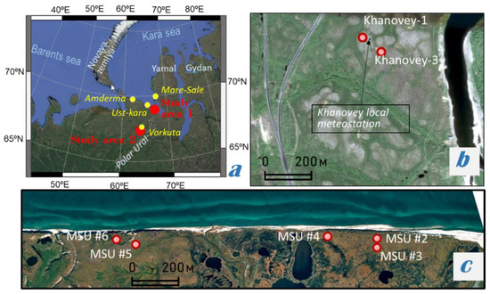
Figure 1.
Location of the research area: (a) satellite image of Russian Arctic segment within Barents and Kara sea regions (from [28]) (meteorological stations—yellow circles); (b) satellite image of in the Khanovey area with boreholes (red circles); (c) satellite image of coastal zone in the Baydaratskaya Bay section with boreholes (red circles) [29].
2.2. Climate Conditions
The climatic conditions of the Baydaratskaya Bay coastal area are generally governed by the variable quantity of incoming solar radiation, atmospheric circulation, and the complex interactions with the proximal Kara Sea. The annual climate is characterized by long severe winter months with a long duration of snow covering, short transitional seasons—spring and autumn, short cold summers, complete absence in some years of a frost-free period [22]. The annual precipitation generally ranges from 300 to 500 mm. A significant amount of the precipitation comes from July to September, accounting for 30–50% of the annual amount [30]. The wind regime represents a monsoon-like character, with the predominant winds in southerly and northerly directions in winter and summer, respectively [31,32]. The Khanovey area is comparatively warmer than the Baydaratskaya Bay area. The frost-free period is about 70 days, while the duration of winter is about eight months.
Snow cover near the coast of the Kara Sea generally starts from the beginning of October, and the mean thickness does not exceed 20 cm. The snow cover gradually grows and reaches its maximum thickness of 60–64 cm in spring (April and May). At the Khanovey site, located far south of the coast, the snow thickness is much greater; its average thickness varies from 18 cm in October to 89 cm in early spring (March–April).
2.3. Geological Settings
In the coastal area of southwestern Baydaratskaya Bay, the thickness of Quaternary deposits reaches up to 150–200 m [33]. Among them, the following main genetic complexes stand out: Upper Pleistocene marine, coastal-marine and alluvial-marine deposits and Holocene marine and coastal-marine deposits [34]. Upper Pleistocene marine and coastal-marine sediments in the coastal zone are represented by loams and clays, alternating in section and plan with fine and fine-grained sands with thin (2–3 mm) interlayers of peat. The study area locates within two present-day geomorphological levels: first sea terrace and laida (tidal flat) with absolute heights of 3–9 m and 0.5–2.5 m, respectively [22]. The sea terrace deposits are mainly composed of medium-fine-grained sands with an admixture of silty and clay particles. Loams often contain peat, pebbles and gravel. Laida deposits consist of silty sand with interlayers of loam.
In the Khanovey study area, the Quaternary section has a thickness of more than 200 m [33]. This section is the complex of glacial, water-glacial, lacustrine, alluvial, boggy and alluvial-diluvial deposits. In most of the region, Quaternary sediments overlap the denuded surface of Paleozoic and Mesozoic rocks, represented by alternating layers of mudstones, sandstones, and siltstones [35].
2.4. Geocryological Conditions
The Baydaratskaya Bay area locates within the zone of continuous permafrost distribution. In general, the permafrost thickness exceeds 100–180 m in the study area [36]. On the day surface, blind taliks are widespread beneath lakebeds and riverbeds, and along the ice lenses formation, massifs of cooled rocks, and cryopegs. At high geomorphological levels, the average annual soil temperature ranges from −2 to −7 °C before 2015 [22]. The ground temperature at deep depths ranges from −5 to −7 °C on the flat-convex surfaces, individual flat-hilly peat bogs on which the density of the snow cover is maximum, and its thickness is insignificant (up to 0.1–0.3 m). The thickness of permafrost varies widely. The typical thickness for the coastal scarp and laida is 50 m, while the permafrost protrudes in the form of a visor direct from the cliff towards the sea, and for an onshore area, it reaches 140 m at elevations in the relief.
On the other hand, the Khanovey research area locates within the zone of discontinuous permafrost distribution [37]. Soil temperature in the Vorkuta region varies from 0 to −2.0 °C. The discontinuity of permafrost is mainly associated with the hydrological and radiation-thermal conditions of taliks. The dissection of submerged taliks is found more often in subsided areas of subsidence with swampy and lacustrine depressions. Typical permafrost thicknesses in Vorkuta (ca. 30 km northwest of Khanovey) and Inta (ca. 210 km southwest of Khanovey) are 50–100 m and 8–10 m, respectively.
3. Methods
3.1. Air Temperature
Air temperature measurements were made at the meteorological stations of Vorkuta (40 km from Khanovei test site), Mare-Sale (100 km from Baydara test site, east cost of Baydara bay), and Ust-Kara (90 km from Baydara test site, west cost of Baydara bay), Amedrma (230 km from Baydara test site, west cost of Baydara bay). A temperature sensor at a height of 2 m from the surface is located at each polygon to assess the impact of microclimate.
3.2. Snow Cover
The thickness of the snow cover for the test sites in different months was determined at meteorological stations. Snow surveys were also carried out at the sites in April 2021. The frequency of observation points is determined by the areal variability of the snow cover thickness.
Each point is tied to the terrain using GPS. The snow cover study included:
- Determining the degree of coverage of the test site by snow cover;
- Determination of the nature of the occurrence of snow cover on the ground;
- Measuring the thickness of the snow cover;
- Assessment of the condition of the soil under the snow cover;
- Measurement of snow density;
- Calculation of the snow water content;
- Photo documentation.
The determination of the main characteristics of the snow cover was carried out at various geomorphological levels.
At each observation point, an instrumental determination of the thickness and density of the snow cover is made by a mass method, using a snow gauge VS-43. The measuring cylinder of VS-43 was pressed into the snow cover down to the soil surface. Snow cover thickness was read out on the cylinder scale. The snow inside the cylinder was pressed with the piston, to prevent the sampled snow from getting out while pulling the cylinder out from snow cover. Then, the content of the cylinder was weighed. The obtained data on snow cover depth and weight were used for the calculation of snow density and snow water content [38].
3.3. Vegetation Cover
The thermal properties of vegetation covers are necessary parameters for any kind of geocryological assessments and predictive calculations. In fieldwork, it is possible to determine the thermal insulating characteristics of vegetation, and its influence on the temperature regime of soils, by using the temperature wave method. The temperature wave method is based on observations of the reduction in the amplitude of daily temperature fluctuations in different points along the depth of the layered vegetation-earth medium. The mobile thermal conductivity meter (MIT-1) device is used to measure the thermal conductivity vegetation cover and soil. This method is one of the non-stationary methods of measuring the heat transfer coefficient of substances, based on the laws of the initial stage of the temperature field development in a semi-continuous body heated by a constant power source [39].
3.4. Lithology, Composition, and Physical Properties of Soils
Parametric boreholes at different landscape types at the two study sites were drilled: at the Khanovei test site, the total drilled depths of boreholes were about 5 m, at the Baydara test site, they ranged from 5 m to 25 m. The boreholes were located at different landscapes: the top of a hillock and the center of a thermokarst depression in Khanovei, low and high terrace in Baydara (Figure 1). All the boreholes were equipped with the temperature logger strings extending from the deep depths to the annual temperature fluctuation depth, allowing to record changes in the ground soil temperature and the thickness of the active layer.
We obtained 30 and 200 samples from the drill cores at the Khanovey and Baydaratskaya Bay study sites, respectively. We analyzed the samples to study their lithology, composition, and physical properties in the studied areas. The grain size of the soils was analyzed using standard methods (the hydrometer analysis and sieve analysis [40]) to determine lithology at the respective borehole. The water content of frozen soils Wtot (%) was determined by drying at a temperature of 105 °C to constant weight [41]. Soil density ρt (g/cm3) in the laboratory and field conditions was determined by the cutting ring method [41]. The liquid limit and plastic limit were determined by the Vasiliev balance cone method and rolling out a thread of the fine portion of soil, respectively [41]. The relative content of organic matter Ir (%) was determined by the gravimetric method based on determining the weight loss of the sample after calcination at a temperature of 525 °C [42]. The degree of salinity of sediments Dsal (%) was determined from the chemical analysis of water extracts [43]. The freezing point Tbf (°C) was measured in the cooler box by the Tbf-8 controller consisting of the DS18620 digital temperature sensors and the software connecting the sensors and computer by the microlane adapter [43].
3.5. Ground Temperature Measurements
The temperature logger strings installed in the boreholes recorded the temperature of soils at depths of 0.25, 0.5, 0.75, 1.0, 1.5, 2.0, 2.5, 3.0, 4.0 and 5.0 m. The temperature recording was every 12 h. The recorded periods at the respective boreholes were: September 2015–January 2019 at Khanovey-1, September 2015–July 2019 at Khanovey-3, September 2016–December 2018 at the MSU #2, September 2016–December 2018 at the MSU #3, June 2013–September 2015 at the MSU #4, June 2014–January 2018 at the MSU #5, and June 2014–July 2019 at the MSU #6.
We estimated the mean annual ground temperature and the amplitude of surface temperature fluctuations at the respective boreholes in the Khanovey and Baydaratskaya Bay areas. Here, we calculated the mean annual ground temperature at the given borehole t (°C) by averaging the temperature values recorded at the deepest sensor of the borehole:
where t (zd) is the temperature (°C) at the deepest sensor zd of the given borehole recorded at the time i, and n is the number of temperature measurements over the period from late August to early September next year (12.5 months). The amplitude of surface temperature fluctuation (A) at the given borehole was calculated by:
where ti(z0) is the temperature (°C) recorded at the first sensor on the ground surface z0 at the time i. We could compute the amplitude of surface temperature fluctuation A only at the boreholes Khanovey-1, Khanovey-3, MSU #4, and MSU #6 in which their shallowest sensors of thermal strings are set close to the ground surface (0–0.1 m).
Using our ground temperature data, we also estimated the thickness of the active layer of permafrost. The thickness of the active layer by thermometry is estimated by determining the depth at which the temperature is equal to the ground freezing start temperature. At the near-surface depths, because the rocks within the borehole are most likely washed and non-saline, we assumed that the temperature at the onset of ground freezing for silty clays and clays is −0.25 °C and for sands and clay silts −0.1 °C (Figure 2). This method is successfully used to estimate the temperature at other experimental test sites [44].
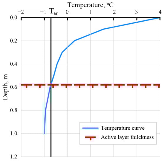
Figure 2.
Determination of the thickness of permafrost active layer for silty clays (Tbf—the temperature of beginning of ground freezing).
3.6. Electrical Resistivity Tomography (ERT)
We carried out the ERT measurements using Russian-made equipment SKALA-64 (NEMFIS, Russia) and SYSCAL Pro 48 (IRIS Instruments, Orleans, France) at the Khanovey and Baydaratskaya Bay coast study sites. The set of equipment includes an ERT station, electrical prospecting streamers, electrodes, and streamer-electrode connectors. We used the measurement protocol of the three-electrode combined setup AMN-MNB (forward and reversed pole-dipole sequence) during the work [45]. The infinity electrode was located perpendicular to each profile at a distance of about 600–800 m, which excluded its influence. The measurements were made at a current of 30–70 mA and a generator voltage of 75 mV. Positioning geophysical profiles and referencing physical observation points were done using differential GPS receivers Trimble R8.
Calibration of electrical tomographic stations is carried out once a year in laboratory conditions on a specialized bench of calibration resistances. In the field, before the research, a control measurement of transient resistances at the electrode-ground contact was carried out. Measurements were made only after reaching acceptable values of transient resistances (about 0.5–1 kOhm). It was done taking into account the dependencies of electric resistivity of rock and sediments on temperature [46].
We processed the ERT data using the two programs X2ipi and Res2dInv (GEOTOMO SOFTWARE, Penang, Malaysia), which provide straightforward processing and interpretation of the results. We used the X2ipi program for processing field data, filtering from noise and random emissions, and integrating the relief data [47]. We used the Res2dInv program for interpreting the two-dimensional data with a semi-automatic mode, taking into account vertical and horizontal inhomogeneities.
4. Results
4.1. Air Temperature
The average annual air temperature drops below freezing, generally falling within −5 and −10 °C. However, the annual air temperatures at all meteorological stations have increased gradually since 2001 (Figure 3). The annual mean air temperature in the Khanovey area is −3.5 °C, which is around 3.5 °C higher than in the Baydaratskaya Bay coast area (−7.0 °C).
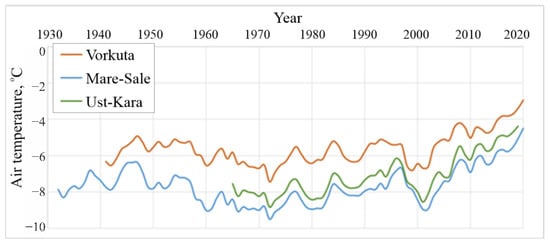
Figure 3.
Annual mean air temperature (5-year averaging) at three meteorological stations: Vorkuta, Mare-Sale, and Ust-Kara (see Figure 1 for their locations).
The microclimate of the test sites is very close to meteorological station data (Figure 4).
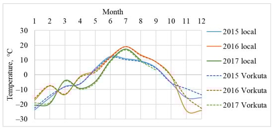
Figure 4.
Comparison of the variation of mean monthly air temperatures according to the data of Vorkuta weather station and microclimatic observations at the Khanovey test site.
4.2. Snow Cover
In 2013–2020, the mean thickness of snow cover near the coast of the Kara Sea was only about 5 cm, and its maximum did not exceed 30 cm (Figure 5). A strong gusty wind prevails in this region, which prevents the gradual accumulation of snow near the coast, and lingering snow on the steep slopes and the surface of sea terraces. According to a snow survey, snow accumulates on the surface of the block-mounds (0 to 0.3 m). Snow cover density varies from 0.35 to 0.45 kg/m3.
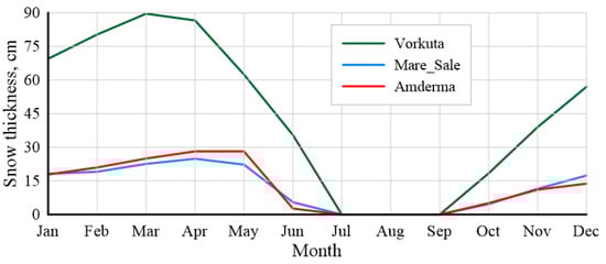
Figure 5.
Annual snow cover thickness (average for 2013–2020) at three meteorological stations: Vorkuta, Mare-Sale, and Amderma.
At the Khanovey site, located far south of the coast, the snow thickness is much greater than 90 cm (Figure 5). The higher snow accumulation is present typically in depressions in the relief, runoff troughs, and stream mouths, and its maximum thickness often reaches several meters according to records at the Vorkuta meteorological station. According to a snow survey, snow accumulates on the surface of the block-mounds (0.2 to 0.5 m). However, even here, the difference of air and earth surface temperatures reaches 3 degrees. In shallow depressions, there is relatively little snow due to the possibility of it being blown out by powerful winds; the difference of air and earth surface temperatures here reaches 4 degrees. In the interblock-extended depressions, snow accumulation is significantly greater and the earth surface temperature is close to zero. In waterlogged areas, with a snow cover thickness of more than one meter, seasonal freezing may not take place. Snow cover density varies from 0.22 to 0.41 kg/m3.
4.3. Vegetation Cover
At the Khanovey site, vegetation is represented by yernik and willow-yernik shrubby-mossy tundras—characteristic communities of the yernik band of the southern tundra. The river valley is dominated by low yernik shrub-lichen tundra, with dwarf semiboreal shrubs (dwarf birch is 20–30 cm tall) and shrubs, combined with small areas of shrub-lichen tundra with Arctic-alpine shrubs, mosses and lichens in the highest parts of the terrain. In the river valley, there are isolated small, mostly overgrown sedge-sphagnum bogs in inter-hilly depressions, and isolated small thermokarst lakes, merging towards the zone of influence of the railroad facilities. Vegetation cover thickness varies from 5 to 20 cm, thermal conductivity ranges from 0.13 to 0.35 W/(m·K).
At the Baydaratskaya Bay site, vegetation is represented by peat. Vegetation cover thickness varies from 20 to 80 cm, thermal conductivity ranges from 0.55 to 0.74 W/(m·K).
4.4. Lithology, Composition, and Physical Properties of Soils
At the Baydaratskaya Bay site, we could describe the following units, from top to bottom in meters below the surface (mbs):
Unit 1 (0–0.5 mbs): Peat. The water content Wtot ranges between 200 and 270%, and the soil density ρt ranges between 1.10–1.22 g/cm3. The stratum is heterogeneous, and there is a clear separation in color. The relative content of organic matter Ir is 65%.
Unit 2 (0.5–3 mbs): Brown loam. The water content Wtot ranges between 33 and 42%, and the soil density ρt ranges between 1.60–1.65 g/cm3 (Figure 6). The plastic limit and liquid limit are 19% and 23%, respectively. Silt particles (0.05–0.002 mm) prevail in grain size (60%). The relative content of organic matter Ir is 5%.
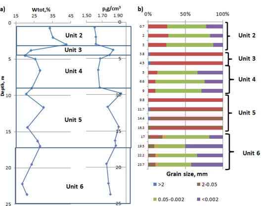
Figure 6.
Characteristics of frozen soils at the Baydaratskaya Bay study site: (a) water content Wtot and soil density ρt vs. depths, (b) grain size vs. depth.
Unit 3 (3–4.5 mbs): Brown silty medium (fine) sand. The water content Wtot ranges between 20 and 23%, and the soil density ρt ranges between 1.80–1.84 g/cm3 (Figure 6). Sand particles (0.25–0.5 mm) prevail in grain size (40%).
Unit 4 (4.5–9 mbs): Grey silty clay. The water content Wtot ranges between 23 and 28%, and the soil density ρt ranges between 1.65–1.67 g/cm3 (Figure 6). The plastic limit and liquid limit are 17% and 28%, respectively. Silt particles (0.05–0.002 mm) prevail in grain size (62%).
Unit 5 (9–16.5 mbs): Grey silty medium (fine) sand. The water content Wtot ranges between 19 and 27%, and the soil density ρt ranges between 1.80–1.94 g/cm3 (Figure 6). Sand particles (0.25–0.5 mm) prevail in grain size (36%).
Unit 6 (16.5–25 mbs): Grey silty clay. The water content Wtot ranges between 17 and 22%, and the soil density ρt ranges between 1.78 and 1.87 g/cm3 (Figure 6). The plastic limit and liquid limit are 19% and 30%, respectively. Silt particles (0.05–0.002 mm) prevail in grain size (47%). This unit contains saline soils (Dsal > 0.5%).
At the Khanovey study site, we could describe the following units, from top to bottom:
Unit 1 (0–0.2 mbs): Vegetation cover.
Unit 2 (0.2–2 mbs): Brown loam. The water content Wtot ranges between 20 and 28%, and the soil density ρt ranges between 1.70–1.75 g/cm3. The plastic limit and liquid limit are 14% and 20%, respectively.
Unit 3 (2–3 mbs): Brown fine sand. The water content Wtot ranges between 12 and 15%, and the soil density ρt ranges between 1.90–1.94 g/cm3.
Unit 2 (3–4.5 mbs): Brown loam. The water content Wtot ranges between 20 and 28%, and the soil density ρt ranges between 1.70–1.75 g/cm3. The plastic limit and liquid limit are 14% and 20%, respectively. There are lenses of fine sand (0.1–0.2 m).
4.5. Ground Temperature Measurements
Mean annual ground temperature t (°C) from all the boreholes calculated for the Khanovey and Baydaratskaya Bay test sites is shown in Figure 7. As for the seasonal amplitude of the surface temperature fluctuation A (°C), we could determine it only at the boreholes Khanovey-1, Khanovey-3, MSU #4, and MSU #6 that had their shallowest sensor close to the surface within the depths of 0–0.1 m.
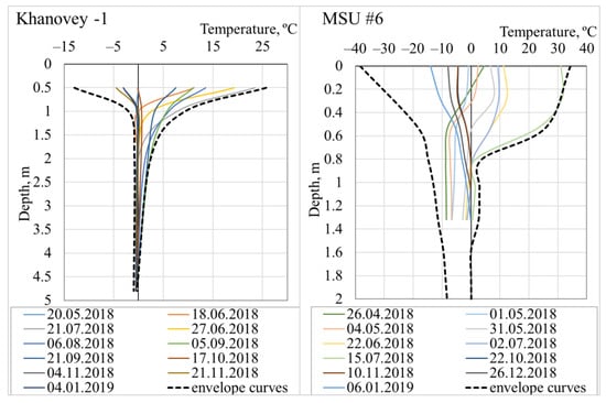
Figure 7.
Ground temperature at the borehole Khanovey-1 at the Khanovey test site and the borehole MSU #6 at the Baydaratskaya Bay test site.
The amplitudes of surface temperature fluctuation A (°C) at the boreholes Khanovey-1, Khanovey-3, MSU #4, and MSU #6 were 39.3 °C, 33.8 °C, 23.9 °C, and 36.4 °C, respectively, representing no significant differences between the Khanovey and Baydarastkaya Bay study sites. On the other hand, the average annual ground temperatures t (°C) at the boreholes MSU #4, and MSU #6 at the Baydaratskaya Bay study site were −3.5 °C, −3.4 °C, respectively (Table 1). The Khanovey study site showed the higher mean annual ground temperatures of −0.5 °C and −0.1 °C at the Khanovey-1 and Khanovey-3 boreholes, respectively (Table 1), indicating their close locations to the boundary of the permafrost zone. We also estimated the thickness of the seasonal thawing layer at the respective wells at the study sites in light of these ground temperature data (Figure 8).

Table 1.
Results of the mean annual temperature and amplitude of temperature fluctuation.
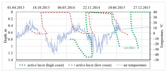
Figure 8.
Changes of active layer thickness at the boreholes: MSU #4 and #6.
In the borehole MSU #6, at the high coast of the Baydaratskaya Bay study site, we could acquire the ground temperature data recordings during June 2014 and July 2019. We could also observe that the periods of the presence of the thawing active layer and its thickness in 2015, 2016, 2017, and 2018 at the MSU#6 site were 151, 159, 135 and 174 days, respectively. The active layer thickness varies from 50 to 130 cm (Figure 9). It indicates that the periods of the thawing active layer were extending year by year due to the steep extension of the warm-season period duration with preservation of air temperature annual amplitudes.
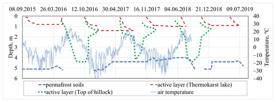
Figure 9.
Changes of active layer thickness and depth of permafrost at the boreholes Khanovey-1 and 3 (air temperature was recorded from our local temperature sensor).
Ground temperature measurements have been made since June 2013 at the borehole MSU #4 located on the low coast in the Baydaratskaya Bay area. At the beginning of the temperature monitoring in 2013, the thickness of the active layer was 40 cm. It then increased by 64 cm around the 19th of September 2013. Our data suggested that freezing started in the second half of October (around 16 October), and the low coast area froze completely around the 4th of December 2013. The active layer began to form again on the 10th of May 2014. The active layer increased to 68 cm in summer 2015 (Figure 8). The borehole MSU#4 was subject to damage in 2015 due to the dramatically rapid coastal retreat.
The borehole Khanovey-1 locates on a damp, flat surface at the Khanovey test site. The vegetation is represented by lichen and dwarf birch up to 20 cm. The data acquisition at the Khanovey-1 well started on 8 September 2015 (Figure 9). The seasonal thawing layer at that time was 3.2 m. Then, when a cold snap came, it began to freeze from 1 October 2015. In addition, the active layer began to freeze from below from 13 October. It completely froze on 5 January 2016. In 2016, the soils began to thaw in mid-May. By 18 August, the active layer reached its maximum thickness of 4.5 m, as suggested by our ground temperature data. It began to shrink from both the top and bottom in the second half of October, and it completely froze on 6 January 2017 (Figure 9).
In 2017, the active layer began to thaw at the end of May 2017. It reached a depth of 1.8 m by 8 June, and this boundary was stable until the end of August (Figure 9). However, before the beginning of September, the thickness of the active layer increased to 4.0 m. Starting from 10 October, it began to freeze through on both sides, as seen in the preceding years. On 11 January, it completely froze. At the end of May 2018, the active layer again began to grow, and it reached its maximum thickness of 4.3 m by 5 September. In the second half of October, it began to freeze again. In November, its thickness reduced by more than half. It completely froze on 4 January 2019 (Figure 9).
The borehole Khanovey-3 was in an overgrown thermokarst lake with an underlying blind talik. Its depth varied depending on the season, shown by the temperature data. In contrast to the micro-district of the borehole Khanovey-1, seasonal freezing occurs here (Figure 10). Measurements of the temperature showed that the permafrost table could rise to 4 m in winter and drop below 5 m in summer. At the same time, the upper layer froze from above only to a depth of 1.4 m. Thus, these results suggest that non-frozen soils constantly exist in this study area, with a thickness of 1.4–4 m.
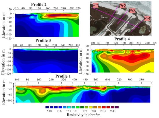
Figure 10.
Results of ERT images in the Baydaratskaya Bay area: Profile #1; Profile #2; Profile #3; Profile #4 and lines of Profiles #1–4 (satellite image from [28]).
4.6. Electrical Resistivity Tomography (ERT)
When field work was performed, the following values were set in the instrumental settings for measurements: performing up to 6 iterations of measurements on each dipole until the error was less than 5%. Further, in the x2ipi data visualization and analysis program, points were discarded—so-called “outliers”. These measures made it possible to obtain smooth apparent resistivity sections (pseudo-section) with minimal errors. However, it should be noted that when performing a two-dimensional data inversion and obtaining a geoelectric cross-section, the root-mean-square deviation of the obtained geoelectric model had a specific electrical resistance (SER) up to a few tens of percentages. Despite such fairly high values, this is a common case, where the specific electrical resistance (SER) of the layers in the section differ from each other by several orders of magnitude. The 2D inversion algorithm does not have sufficient dynamic range to fit a smooth geoelectric model with such a high resistivity gradient. Nevertheless, it should be noted that just the areas where a sharp increase in recorded specific electrical resistance (SER) values clearly indicate a change in the state of the soil (thawed-frozen).
Our ERT measurements in the Baydaratskaya Bay area were carried out in the four Profiles #1–4 at the Cofferdam site in September 2017 (Figure 10). One longitudinal coastal Profile #1, located at 180–200 m landward from the sea, was 945 m long, consisting of 3 electro-tomography layouts of 315 m each. Profile #1 crosses the first sea terrace and laida. Profile #2 transects the beach, slope and the first sea terrace. Profile #3 runs through the laida (the height of the laida is 0.8–1 m) and the beach. Profile #4 crosses a small part of the beach, a high cliff (10 m high), and the first sea terrace. The distance between Profiles #3 and #4 was approximately 1 km. Specific electrical resistance in our ERT measurements in the Profiles #1–4 varied from 5 to 6000 Ω·m. The resistivities for permafrost and unfrozen soils (thawed and saline) ranged from 500 to 5500 Ω·m and from 5 to 500 Ω·m, respectively. In general, the resistivity in the western area is considerably higher than that in the eastern one. It indicates that this area has thawed saline soils, and that the thickness of the permafrost varies widely from the first 10′s of meters to 100′s meters. These interpretations may not be unique because there are saline soils and cryopegs in this coastal area, which significantly affect the resistivity and state of frozen soil [26,27].
We carried out the ERT measurement in the Khanovey field station in 2019. The profile runs for 280 m from northwest to southeast (Figure 11). Specific electrical resistance in the ERT profile varied from 5 to 3000 Ω·m. The permafrost thickness in this area is 40–90 m [16]. In this area, we observed the distribution of frozen soils in the upper part of the section independent of the relief and the presence of water cover. From our ERT images, frozen soils locate under local rises. In the depressions, where water is stored and the greatest thickness of snow is observed, thawed soils or taliks can form [16]. We interpreted the zones with the resistivities showing lower than 300 Ω·m, ranging between 300 and 500 Ω·m, higher than 500 Ω·m as the zones of unfrozen ground, talik, and permafrost, respectively.
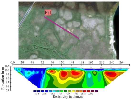
Figure 11.
Results of ERT images in the area of Khanovey station (satellite image from [28]).
5. Discussion
5.1. Air Temperature
Air temperature is the main parameter for thermal modeling. Data of regional me-teorological station can be used. Besides, a detailed archive of many hydrometeorological parameters with a spatial resolution of less than 5 km in the Russian Arctic allows us to obtain a regional non-hydrostatic model (COSMO-CLM). It can be used for microclimate evaluation [48]. However, it is necessary to have an air temperature sensor at the test site for comparison data.
5.2. Snow Cover
In addition to an increasing average annual air temperature, there is also an increasing quantity of precipitation, which in the permafrost leads to an increasing thickness of the snow cover, and as result, rising active layer depth and reduction of permafrost distribution. There are insignificant snow cover changes at the Baydara test site. However, at the Khanovey test site, the thickness of the snow cover is one of the main factors that must be taken into account in this region. So, in 2016, the average annual snow thickness was 131 mm (maximum 370 mm), and in 2017 almost 3 times more—368 mm (maximum 910 mm). At the same time, the average annual temperature in 2016 was 2 °C higher than in 2017. That is why the active layer depth changes not more than 20%.
5.3. Vegetation Cover
At the Baydara test site, the vegetation cover is uniform and is represented by peat (from 20 to 80 cm). At the Khanovey test site, the vegetation cover can be divided into four groups.
(1) The flat-topped hill surfaces are occupied by most cold-loving communities of the more northern territories shrub-lichen tundra with isolated occurrences of dwarf birch with the lowest height and foliage projective cover (15–25%, average—17%). Communities of shrub-lichen tundra, gravitate towards the most elevated, wind-exposed areas of flat-topped hill structures, with the greatest temperature fluctuations and are characterized by the lowest height of all layers of vegetation (lichens—2–4 cm, shrubs—15–20 cm, ground shrubs—2–4 cm).
(2) On the slopes of the flat-topped hill structures, low yernik shrub-lichen tundra dominates, being replaced, along the slope, by moss-lichen and lichen-moss tundra. There is an increase in the abundance (from 12–15% to 45–70%) and height (from 17–20 cm to 30–35 cm) of dwarf birch on the slopes of flat-topped hill structures in the low yernik shrub-lichen tundra.
(3) In the inter-hill depressions, there is a predominance of yernik shrubby-sedge-moss tundra with the highest projective cover of the shrub layer (70–85%) with a predominance of dwarf birch (50–90 cm, up to 120 cm in height) and maximum moss as ground cover (80–95%) of red-stemmed feathermoss and glittering wood moss 8–10 cm in height, which levels out temperature fluctuations and reduces penetration of daily fluctuations into the ground.
(4) In inter-hill depressions, there are isolated small areas (approx. 5 × 3 m) of sedge-sphagnum bogs.
The coefficient of thermal conductivity of the vegetation cover can differ by a factor of 4 for these two sites.
5.4. Lithology, Composition, and Physical Properties of Soils
Determination of the composition and properties of the soil is necessary for the verification and calibration of thermal modeling. In addition, the data are used for the interpretation of electrical resistivity tomography and ground temperature measurements. The next step is the determination the thermal properties of soils in frozen and thawed states [34]. However, it is also possible to use table values for the thermal properties depending on water content and density [49]. Temperature and salinity impact all properties of frozen soil [50]. That is why it is so important to have these data for the Baydara test site.
5.5. Ground Temperature
The average annual temperature of soils on the high and low coast of the Baydaratskaya Bay field station did not differ so much between the boreholes (Table 1). The amplitude of temperature fluctuation near the high coast was 36.4 °C, low coast was 23.9 °C. The temperatures of the soils are close to each other. This is due to their close locations to the edge of the slopes, where the thermal effect occurs both vertically and along the slope line. This coastal section retreated by 1.0–1.9 m per year in 2005–2016 [22].
The temperature of the soil at the Khanovey test site was much higher than that at the Baydaratskaya Bay study site (Figure 3). The hillocks had a soil temperature of −0.5 °C and an amplitude of temperature fluctuation in the surface temperature of 39.3 °C (Table 1). In the inter-mound depressions, and in particular, the thermokarst lake, the mean annual ground temperatures were close to the temperature at the onset of rock freezing of −0.1 °C. The amplitude of temperature fluctuation at the thermokarst lake was 33.8 °C. In general, the amplitude of temperature fluctuation at the Khanovey study site was higher than that at the Baydaratskaya Bay site, suggesting that the distance from the sea and the influence of the continental climate effect are primary factors.
At the Khanovey site, the layer of seasonal thawing was much larger, varying from 3.2 to 4.4 m, judged by the data from the Khanovey-1 borehole. In the Khanovey-3 borehole, the situation is different. It locates on an overgrown thermokarst lake with a suspected talik, and it thus did not freeze completely. Only seasonal freezing occurs here, and its depth was from 0.8 m to 1.4 m in the studied period. Due to the large active layer thickness, the standard probe method does not work at this test site. Only ground temperature data or electrical resistivity tomography can be used.
The time of the formation of the active layer and its subsequent decrease at both study sites was similar, ranging from May to October. The seasonal freezing layer forming at the borehole Khanovey-3 has a similar time frame, from October to May. However, the nature of freezing the seasonally thawed layer is very different between the study sites. At the Khanovey research site, closure occurred on average at a depth of 1.5 m, which was half of the entire thickness of the seasonally thawed layer. Contrastingly, at the Baydaratskaya Bay site, the seasonal thawing layer closes only due to freezing from above and at the same depth as the base of the seasonally thawed layer.
Mean annual ground temperature and amplitude of surface temperature fluctuation can be used for analytical calculations [51] and harmonic analyses [52].
5.6. Electrical Resistivity Tomography (ERT)
Very few publications report the subsurface ERT images along the permafrost coasts worldwide [53,54,55], and thus, the permafrost structure along the southwest coast of the Baydaratskaya Bay is poorly understood. In our ERT measurements, an interelectrode pitch of 5 m was chosen, with a total string profile length of 315 m. The maximum length of the ERT interpretation profile was about 280 m. The resulting vertical resolution in the upper part of the section was 1.5–2 m. Although it was difficult to estimate the active layer thickness, which is less than 1 m on average at the entire site well below the vertical resolution, it was possible to identify talik zones and the permafrost base.
Frozen soils are imperfect dielectrics and characterized by their high resistivity values. In the frozen state, the resistivity of dispersed soils is 10 to 100 times higher than that of the same soils in the thawed state [56]. In addition, the resistivity of frozen rocks is influenced by the lithological composition, moisture content, ice content, cryogenic structure, temperature and mineralization of the pore solution. For example, the resistivity in finely dispersed soils with a massive cryogenic texture increases by 10–100 times, up to 400–5000 times with the formation of a schlieren cryogenic texture and ice wedges [57].
Our interpretation of the electric exploration sections without considering the effect of salinity could be as follows: frozen soils with resistivity above 500 Ω·m and thawed soils with resistivity below 500 Ω·m. However, we recognize that saline soils have a significant effect on their resistivity [58]. They are manifested in geoelectric sections by a sharp decrease in resistivity, and the dependence of resistivity on lithology and temperature acquires a specific character. Nevertheless, with a high degree of salinity of frozen soils, the resistivity values practically do not differ from the thawed ones [59]. In this regard, the interpretation of the results could have great uncertainty since the salinity at depths of more than 30 m is unknown.
Profile No. 1 is 945 m long, runs through the first sea terrace and laida, paralleling to the coast (Figure 7). On the side of the sea terrace, at the depth from 0.6–1 m to 30–45 m, we observed high resistivity values near the constituent rock strata. We concluded that the permafrost thickness here averages 30–40 m, and its maximum reaches locally 60 m in this study area. Based on Profiles No. 1 and No. 3, we suggest that permafrost is completely absent in the territory of the entire laida. The resistivity of the rocks here averages about 100 Ω·m, indicative of the presence of thawed rocks or cooled saline soils. The low laidas in this area are often flooded, contributing to the saltwater infiltration and thawing of the ground.
Profile No. 2 locates perpendicular to the seashore and crosses Profile No. 1 (Figure 7). The resistivity of rocks beneath the beach and the adjacent slope varied from 5 to 40 Ω·m at the depths of 1 to 15 m. This result indicates a thawed state and/or the presence of cooled saline soils. The profile image further suggests that there is a permafrost boundary at a distance of approximately 170 m from the water’s edge. The permafrost thickness is 20–25 m. The depth of the permafrost roof on the terrace varies from 3–3.5 m to 4–4.5 m, and then deepens slightly to 5.5 m associated with the presence of the lake.
Profile No. 4 crosses the beach, the slope (ca. 6 m high), and the sea terrace. High resistances in this area are observed, starting from the upper edge of the slope to further upward of the slope continuously (Figure 7). The position of the permafrost base reaches a depth of 85 m. Concurrently, we also observed a layer with low resistivity values at a depth of 13 m to 25 m, extending from the cliff to the terrace. The same low resistances are found throughout the section. This fact can be explained by the fact that this layer contains saline cooled dispersed soils. Our interpretation of permafrost suggested by ERT data is consistent with the ground temperature data representing temperatures below the freezing point.
Compared with the Baydaratksya Bay area, the interpretation of our ERT image in the Khanovey area can be unique because the soils are not saline.
Despite the difference in air temperature, snow cover thickness, soil properties, the thickness of the permafrost is almost the same for the two sites and varies from 0 to 90 m. However, the reasons for the formation of uneven permafrost distribution are completely different. At the Baydaratskaya Bay test site, taliks are located on the beach, where the sea has a warming effect. At the Khanovei test site, taliks were formed due to the uneven distribution of snow.
6. Conclusions
We have proposed a novel multi-parameter monitoring protocol, which consists of the following set of controlled parameters:
- Air temperature;
- Snow cover (thickness, density, thermal conductivity);
- Vegetation cover (classification, thickness, thermal conductivity);
- Soil properties (classification, grain size, water content, density, Attenberg limits, the relative content of organic matter, salinity, freezing point);
- Permafrost distribution (talik sizes);
- Mean annual ground temperature;
- Amplitude of surface temperature fluctuations;
- Thickness of the active layer;
- Type of cryogenic processes.
These parameters were compiled on the basis of the principles of a complete characterization of the geocryological conditions of the test site, functioning the monitoring system based on the developed protocol, and frequency of measurements. By integrating the study of the composition and properties of soils, soil temperatures, electrical resistance of frozen and thawed grounds, our work allowed us to fully characterize the studied sites, suggesting that it will help further monitoring in the future and in the modeling of the thermal state in the European north of Russia, and also assist in the calibration of remote sensing data such as Synthetic Aperture Radar Interferometry (InSAR) [60]. Our test sites made it possible to focus stationary observations on the typical areas in the European part of the Russian Arctic that were identified at the preliminary stage of the study. This will allow applying the received monitoring materials in territories with a similar set of conditions. Our general multi-parameter monitoring protocol may be supplemented with specific methods to monitor cryogenic processes or infrastructure facilities.
Author Contributions
Conceptualization, V.I. and P.K.; methodology, D.O.S., P.K., A.K. (Andrey Koshurnikov) and O.K.; software, O.K.; validation, A.K. (Arata Kioka), A.U. and P.K.; formal analysis, O.K. and A.U.; investigation, V.I., O.K. and D.O.S.; resources, A.K. (Andrey Koshurnikov); data curation, A.K. (Arata Kioka) and P.K.; writing—original draft preparation, P.K. and V.I.; writing—review and editing, A.K. (Arata Kioka), V.I. and P.K.; visualization, O.K. and A.U.; supervision, V.I.; project administration, V.I.; funding acquisition, A.K. (Arata Kioka), P.K. and V.I. All authors have read and agreed to the published version of the manuscript.
Funding
This research was funded by the grant RFBR, No 21-55-50012 and Japan-Russia Research Cooperative Program between JSPS and RFBR (JPJSBP120214811).
Institutional Review Board Statement
Not applicable.
Informed Consent Statement
Not applicable.
Data Availability Statement
Not applicable.
Acknowledgments
The authors express their gratitude to North Direction of Russian railway, JSC GazpromTransGas Uhta and Vernadsky Institute of Geochemistry and Analytical Chemistry of RAS for administrative and technical support. The authors would also like to thank the reviewers and the editor for their helpful comments on an earlier version of the manuscript. This work is supported by the grant RFBR, No 21-55-50012\21 and Japan-Russia Research Cooperative Program between JSPS and RFBR (JPJSBP120214811) and Vernadsky Institute of Geochemistry and Analytical Chemistry of RAS.
Conflicts of Interest
The authors declare no conflict of interest. The funders had no role in the design of the study; in the collection, analyses, or interpretation of data; in the writing of the manuscript, or in the decision to publish the results.
References
- Obu, J.; Westermann, S.; Bartsch, A.; Berdnikov, N.; Christiansen, H.H.; Dashtseren, A.; Delaloye, R.; Elberling, B.; Etzelmüller, B.; Kholodov, A.; et al. Northern Hemisphere Permafrost Map Based on TTOP Modelling for 2000–2016 at 1 km2 Scale. Earth Sci. Rev. 2019, 193, 299–316. [Google Scholar] [CrossRef]
- Yershov, E.D. General Geocryology (Studies in Polar Research); Williams, P., Ed.; Cambridge University Press: Cambridge, UK, 1998. [Google Scholar] [CrossRef]
- Biskaborn, B.K.; Smith, S.L.; Noetzli, J.; Matthes, H.; Vieira, G.; Streletskiy, D.A.; Schoeneich, P.; Romanovsky, V.E.; Lewkowicz, A.G.; Abramov, A.; et al. Permafrost is warming at a global scale. Nat. Commun. 2019, 10, 264. [Google Scholar] [CrossRef] [PubMed] [Green Version]
- Romanovsky, V.E.; Smith, S.L.; Isaksen, K.; Nyland, K.E.; Kholodov, A.L.; Shiklomanov, N.I.; Streletskiy, D.A.; Farquharson, L.M.; Drozdov, D.S.; Malkova, G.V.; et al. Terrestrial Permafrost. In State of the Climate in 2019. Bull. Am. Meteorol. Soc. 2020, 101, 265–271. [Google Scholar] [CrossRef]
- Jin, X.-Y.; Jin, H.-J.; Iwahana, G.; Marchenko, S.S.; Luo, D.-L.; Li, X.-Y.; Liang, S.-H. Impacts of climate-induced permafrost degradation on vegetation: A review. Adv. Clim. Change Res. 2020, 12, 29–47. [Google Scholar] [CrossRef]
- Stephen, K. Societal Impacts of a Rapidly Changing Arctic. Curr. Clim. Change Rep. 2018, 4, 223–237. [Google Scholar] [CrossRef] [Green Version]
- Ramage, J.; Jungsberg, L.; Wang, S.; Westermann, S.; Lantuit, H.; Heleniak, T. Population living on permafrost in the Arctic. Popul. Environ. 2021, 43, 22–38. [Google Scholar] [CrossRef]
- Hjort, J.; Karjalainen, O.; Aalto, J.; Westermann, S.; Romanovsky, V.E.; Nelson, F.E.; Etzelmüller, B.; Luoto, M. Degrading permafrost puts Arctic infrastructure at risk by mid-century. Nat. Commun. 2018, 9, 5147. [Google Scholar] [CrossRef]
- Streletskiy, D.A.; Suter, L.J.; Shiklomanov, N.I.; Porfiriev, B.N.; Eliseev, D.O. Assessment of climate change impacts on buildings, structures and infrastructure in the Russian regions on permafrost. Environ. Res. Lett. 2019, 14, 025003. [Google Scholar] [CrossRef]
- Melnikov, V.P.; Osipov, V.I.; Brouchkov, A.V.; Falaleeva, A.A.; Badina, S.V.; Zheleznyak, M.N.; Sadurtdinov, M.R.; Ostrakov, N.A.; Drozdov, D.S.; Osokin, A.B.; et al. Climate warming and permafrost thaw in the Russian Arctic: Potential economic impacts on public infrastructure by 2050. Nat. Hazards 2022, 21. [Google Scholar] [CrossRef]
- Miner, K.R.; Turetsky, M.R.; Malina, E.; Bartsch, A.; Tamminen, J.; McGuire, A.D.; Fix, A.; Sweeney, C.; Elder, C.D.; Miller, C.E. Permafrost carbon emissions in a changing Arctic. Nat. Rev. Earth Environ. 2022, 3, 55–67. [Google Scholar] [CrossRef]
- Turetsky, M.R.; Abbott, B.W.; Jones, M.C.; Anthony, K.W.; Olefeldt, D.; Schuur, E.A.G.; Grosse, G.; Kuhry, P.; Hugelius, G.; Koven, C.; et al. Carbon release through abrupt permafrost thaw. Nat. Geosci. 2020, 13, 138–143. [Google Scholar] [CrossRef]
- Smith, S.; Brown, J. Assessment of the Status of the Development of the Standards for the Terrestrial Essential Climate Variables. Permafrost and Seasonally Frozen Ground. 2009. Available online: http://library.arcticportal.org/668/ (accessed on 17 January 2022).
- Circumpolar Active Layer Monitoring Network (CALM). Soil Moisture Content. Available online: https://www2.gwu.edu/~calm/research/soil_moisture.html (accessed on 17 January 2022).
- Domine, F.; Belke-Brea, M.; Sarrazin, D.; Arnaud, L.; Barrere, M.; Poirier, M. Soil moisture, wind speed and depth hoar formation in the Arctic snowpack. J. Glaciol. 2018, 64, 990–1002. [Google Scholar] [CrossRef] [Green Version]
- Nelson, F.E.; Hinkel, K.M.; Humlum, O.; Matsuoka, N. (Eds.) A Handbook on Periglacial Field Methods. 2004. Available online: https://ipa.arcticportal.org/publications/handbook (accessed on 17 January 2022).
- Arctic Development and Adaptation to Permafrost in Transition (ADAPT). ADAPT Standard Protocols. Available online: http://www.cen.ulaval.ca/adapt/protocols/adapt.php (accessed on 17 January 2022).
- Doré, G.; Niu, F.; Brooks, H. Adaptation Methods for Transportation Infrastructure Built on Degrading Permafrost. Permafr. Periglac. Process. 2016, 27, 352–364. [Google Scholar] [CrossRef]
- Hart, J.D.; Powell, G.H.; Hackney, D.; Zulfiqar, N. Geometry monitoring of the Trans-Alaska pipeline. In Cold Regions Engineering: Cold Regions Impacts on Transportation and Infrastructure; 2002; pp. 110–121. Available online: http://www.ssdinc.com/documents/PiggingPaper_ColdRegions2002.pdf (accessed on 10 January 2022).
- Ran, Y.; Li, X.; Cheng, G. Climate warming over the past half century has led to thermal degradation of permafrost on the Qinghai–Tibet Plateau. Cryosphere 2018, 12, 595–608. [Google Scholar] [CrossRef] [Green Version]
- STO Gazprom 2-3.1-072-2006. “Regulations for Geotechnical Monitoring of Engineering Facilities of the Gas Complex in the Permafrost Zone” Gasprom, p. 61. Available online: https://www.russiangost.com/p-305996-sto-gazprom-2-31-072-2006.aspx (accessed on 10 January 2022).
- Isaev, V.; Koshurnikov, A.; Pogorelov, A.; Amangurov, R.; Podchasov, O.; Sergeev, D.; Buldovich, S.; Aleksyutina, D.; Grishakina, E.; Kioka, A. Cliff retreat of permafrost coast in south-west Baydaratskaya Bay, Kara Sea, during 2005–2016. Permafr. Periglac. Process. 2019, 30, 35–47. [Google Scholar] [CrossRef]
- Dmitry, S.; Anisimov, O.; Vasiliev, A. Permafrost Degradation. 2008; pp. 1305–1310. Available online: https://www.researchgate.net/publication/268504716_Permafrost_Degradation (accessed on 10 January 2022).
- Vasiliev, A.A.; Drozdov, D.S.; Gravis, A.G.; Malkova, G.V.; Nyland, K.E.; Streletskiy, D.A. Permafrost degradation in the Western Russian Arctic. Environ. Res. Lett. 2020, 15, 045001. [Google Scholar] [CrossRef]
- The Ministry of Natural Resources and the Environment of the Russian Federation. An Informational Report with an Assessment of the Current State Natural and Technogenic Situation of the Russian Arctic [Including Mare-Sale and Vorkuta Test Sites]. 2019. Available online: https://geomonitoring.ru/download/pshz/arctic2018.pdf. (accessed on 17 January 2022). (In Russian).
- Kotov, P.I.; Khilimonyuk, V.Z. Building Stability On Permafrost In Vorkuta, Russia. Geogr. Environ. Sustain. 2021, 14, 67–74. [Google Scholar] [CrossRef]
- SP 305.1325800.2017; Buildings and Structures. Rules for Conducting Geotechnical Monitoring during Construction. Standardinform: Moscow, Russia, 2017; p. 86.
- Google Earth. Available online: https://earth.google.com (accessed on 17 January 2022).
- QuickBird-2 Instruments. Available online: https://earth.esa.int/eogateway/missions/quickbird-2 (accessed on 17 January 2022).
- Larin, S.I. (Ed.) Atlas of the Yamal-Nenets Autonomous Region; FSUE “Omsk Cartographic Factory”: Omsk, Russia, 2004; p. 303. [Google Scholar]
- Ogorodov, S.; Arkhipov, V.; Kokin, O.; Marchenko, A.; Overduin, P.; Forbes, D. Ice Effect on Coast and Seabed in Baydaratskaya Bay, Kara Sea. Geogr. Environ. Sustain. 2013, 6, 21–37. [Google Scholar] [CrossRef] [Green Version]
- Pavlov, V.A.; Lebedeva, E.S.; Lakeev, V.G. (Eds.) Kara Sea. In Ecological Atlas; Atlases of the Russian Arctic Seas; Arctic Research Center LLC: Russia, Moscow, 2016; p. 272. ISBN 978-5-9908796-0-7. (In Russian) [Google Scholar]
- Ministry of Natural Resources of the Russian Federation; Federal Agency for Subsoil Use; The Department of Mineral Resources of Northwestern Federal District; FSBI VSEGEI Named after A. P. Karpinsky. State Geological Map of the Russian Federation Scale 1: 200,000 Second Edition, Series Polar-Ural Sheets R-42-XXV, XXVI (Yary). 2018. Available online: https://vsegei.ru/ru/info/pub_ggk200-2/polyarnouralskaya/r-42-xxv-xxvi.php (accessed on 17 January 2022).
- Aleksyutina, D.M.; Motenko, R.G. The composition, structure and properties of frozen and thawed deposits on the Baydaratskaya Bay coast, Kara Sea. Earth’s Cryosphere 2017, 21, 11–22. [Google Scholar] [CrossRef]
- Vladislav, I.; Pavel, K.; Dmitrii, S. Technogenic Hazards of Russian North Railway. In Transportation Soil Engineering in Cold Regions; Lecture Notes in Civil Engineering; Springer: Singapore, 2020; Volume 1. [Google Scholar] [CrossRef]
- Grigoriev, N.F. Cryolithozone of the Coastal Part of Western Yamal; Permafrost Institute: Yakutsk, Russia, 1987; p. 111. [Google Scholar]
- Williams, P.J.; Warren, M.T. The English Language Edition of the Geocryological Map of Russia and Neighboring Republics; Collaborative Map Project, Soft Cover: Ottawa, ON, Canada, 1999; p. 32. ISBN 0-9685013-0-3. Map: 16 Sheets (95 × 66 cm per sheet), Scale 1:2,500,000. [Google Scholar] [CrossRef]
- Hribik, M.; Vida, T.; Skvarenina, J.; Skvareninova, J.; Ivan, L. Hydrological effects of Norway spruce and European beech on snow cover in a mid-mountain region of the Polana mts. Slovakia/Hydrologický vplyv smreka obyčajného a buka lesného na snehovú pokrývku v stredohorských polohách pohoria poľana na slovensku. J. Hydrol. Hydromech. 2012, 60, 319–332. [Google Scholar] [CrossRef] [Green Version]
- Isaev, V.S.; Kotov, P.I.; Khilimonjuk, V.Z. Manual for Vorkuta Fieldwork Activities; Kotov, P.I., Gordeeva, G.I., Eds.; KDU: Moscow, Russia, 2022; p. 200. [Google Scholar]
- GOST 12536-2014. Methods for Laboratory Determination of Particle Size (Grain) and Micro-Aggregate Composition. 2014. Available online: https://docs.cntd.ru/document/1200116022 (accessed on 17 January 2022).
- GOST 5180-2015. Methods for Laboratory Determination of Physical Characteristics. 2015. Available online: https://docs.cntd.ru/document/1200126371 (accessed on 17 January 2022).
- GOST 23740-2016. Methods for Determination of Organic Matter Content. 2016. Available online: https://docs.cntd.ru/document/1200143232 (accessed on 17 January 2022).
- Roman, L.T.; Tsarapov, M.N.; Kotov, P.I.; Volokhov, S.S.; Motenko, R.G.; Cherkasov, A.M.; Stein, A.I.; Kostousov, A.I. A Guide for Determining the Physical and Mechanical Properties of Freezing, Frozen and Thawing Dispersed Soils; KDU: Moscow, Russia, 2018; p. 188. [Google Scholar]
- Uvarova, A.V.; Komarov, I.A.; Isaev, V.S.; Tyurin, A.I.; Bolotyuk, M.M. The Dynamics of the Parameters of the Active Layer. Mosc. Univ. Geol. Bull. 2020, 75, 268–276. [Google Scholar] [CrossRef]
- Hemeda, S. Electrical Resistance Tomography (ERT) Subsurface Imaging for Non-destructive Testing and Survey in Historical Buildings Preservation. Aust. J. Basic Appl. Sci. 2013, 7, 344–357. [Google Scholar]
- Vanhala, H.; Lintinen, P.; Oberman, N.; Jokinen, J. Monitoring Permafrost Degradation with Geophysical Methods. In Report of Year 2009 Studies by the River Ko-Rotaikha, NW Russia; Geological survey of Finland Report, Finland. 2010. Available online: https://www.researchgate.net/publication/351625570_Monitoring_permafrost_degradation_with_geophysical_methods_-_Report_of_year_2009_studies_by_the_river_Korotaikha_NW_Russia (accessed on 10 January 2022).
- Bobachev, A.A. ERT—The method of resistance and induced polarization. Devices Syst. Explor. Geophys. 2006, 2, 14–17. [Google Scholar]
- Platonov, V.; Varentsov, M. Introducing a New Detailed Long-Term COSMO-CLM Hindcast for the Russian Arctic and the First Results of Its Evaluation. Atmosphere 2021, 12, 350. [Google Scholar] [CrossRef]
- State Standard 25 13330:2012; Soil Bases and Foundations on Permafrost Soils. Standardinform: Moscow, Russia, 2012; p. 152.
- Kotov, P.I.; Stanilovskaya, J.Y.V. Predicting changes in the mechanical properties of frozen saline soils. Eur. J. Environ. Civ. Eng. 2021. Available online: https://www.tandfonline.com/doi/full/10.1080/19648189.2021.1916604 (accessed on 10 January 2022). [CrossRef]
- Kudryavtsev, V.A. (Ed.) Basics of Permafrost Forecast in Engineering-Geological Investigations; Moscow University Press: Moscow, Russia, 1974. (In Russian) [Google Scholar]
- Islam, M.A.; Lubbad, R.; Amiri, S.A.G.; Isaev, V.; Shevchuk, Y.; Uvarova, A.V.; Afzal, M.S.; Kumar, A. Modelling the seasonal variations of soil temperatures in the Arctic coasts. Polar Sci. 2021, 30, 100732. [Google Scholar] [CrossRef]
- Farzamian, M.; Vieira, G.; Santos, F.A.M.; Tabar, B.Y.; Hauck, C.; Paz, M.C.; Bernardo, I.; Ramos, M.; de Pablo, M.A. Detailed detection of active layer freeze–thaw dynamics using quasi-continuous electrical resistivity tomography (Deception Island, Antarctica). Cryosphere 2020, 14, 1105–1120. [Google Scholar] [CrossRef] [Green Version]
- Pedrazas, M.N.; Cardenas, M.B.; Demir, C.; Watson, J.A.; Connolly, C.T.; McClelland, J.W. Absence of ice-bonded permafrost beneath an Arctic lagoon revealed by electrical geophysics. Sci. Adv. 2020, 6, eabb5083. [Google Scholar] [CrossRef]
- Kim, K.; Lee, J.; Ju, H.; Jung, J.Y.; Chae, N.; Chi, J.; Kwon, M.J.; Lee, B.Y.; Wagner, J.; Kim, J.-S. Time-lapse electrical resistivity tomography and ground penetrating radar mapping of the active layer of permafrost across a snow fence in Cambridge Bay, Nunavut Territory, Canada: Correlation interpretation using vegetation and meteorological data. Geosci. J. 2021, 25, 877–890. [Google Scholar] [CrossRef]
- Zykov, Y.D. Geophysical Methods for Studying the Permafrost; Moscow University Publishing House: Moscow, Russia, 2007; p. 272. [Google Scholar]
- Wu, Y.; Nakagawa, S.; Kneafsey, T.J.; Dafflon, B.; Hubbard, S. Electrical and seismic response of saline permafrost soil during freeze—Thaw transition. J. Appl. Geophys. 2017, 146, 16–26. [Google Scholar] [CrossRef]
- Koshurnikov, A.V.; Kotov, P.I.; Agapkin, I.A. The Influence of Salinity on the Acoustic and Electrical Properties of Frozen Soils. Mosc. Univ. Geol. Bull. 2020, 75, 97–104. [Google Scholar] [CrossRef]
- Agapkin, I.; Kotov, P. Determination State of Frozen Saline Soils by Geophysical Methods. In Proceedings of the Tyumen, Tyumen, Russia, 22–26 March 2021; pp. 1–6. Available online: https://www.earthdoc.org/content/papers/10.3997/2214-4609.202150012# (accessed on 10 January 2022).
- Rouyet, L.; Karjalainen, O.; Niittynen, P.; Aalto, J.; Luoto, M.; Lauknes, T.R.; Larsen, Y.; Hjort, J. Environmental Controls of InSAR-based Periglacial Ground Dynamics in a Sub-Arctic Landscape. J. Geophys. Res. Earth Surf. 2021, 126, e2021JF006175. [Google Scholar] [CrossRef]
Publisher’s Note: MDPI stays neutral with regard to jurisdictional claims in published maps and institutional affiliations. |
© 2022 by the authors. Licensee MDPI, Basel, Switzerland. This article is an open access article distributed under the terms and conditions of the Creative Commons Attribution (CC BY) license (https://creativecommons.org/licenses/by/4.0/).